Cosmological constraints on the dark energy equation of state and its evolution

Abstract

We have calculated constraints on the evolution of the equation of state of the dark energy, $w(z)$, from a joint analysis of data from the cosmic microwave background, large scale structure and type-Ia supernovae. In order to probe the time-evolution of $w$ we propose a new, simple parametrization of $w$, which has the advantage of being transparent and simple to extend to more parameters as better data becomes available. Furthermore it is well behaved in all asymptotic limits. Based on this parametrization we find that $w(z=0)=-1.43^{+0.16}_{-0.38}$ and $dw/dz(z=0)=1.0^{+1.0}_{-0.8}$. For a constant $w$ we find that $-1.34\leq w\leq-0.79$ at 95% C.L. Thus, allowing for a time-varying $w$ shifts the best fit present day value of $w$ down. However, even though models with time variation in $w$ yield a lower $\chi^{2}$ than pure $\Lambda$CDM models, they do not have a better goodness-of-fit. Rank correlation tests on supernova data also do not show any need for a time-varying $w$.

1 Introduction

The discovery in 1998 [1, 2] that the universal expansion is currently accelerating is one of the most spectacular result in cosmology from the past decade. The finding has since been confirmed by observations of the Cosmic Microwave Background (CMB) [3, 4] and the large scale structure (LSS) of the universe [5, 7, 6]

One possible explanation is that the energy density of the universe is dominated by dark energy with a negative equation of state. The simplest possibility is the cosmological constant which has $P=w\rho$ with $w=-1$ at all times. However, since the cosmological constant has a value completely different from theoretical expectations one is naturally led to consider other explanations for the dark energy.

A light scalar field rolling in a very flat potential would for instance have a strongly negative equation of state, and would in the limit of a completely flat potential lead to $w=-1$ [8, 9, 10]. Such models are generically known as quintessence models. The scalar field is usually assumed to be minimally coupled to matter, but very interesting effects can occur if this assumption is relaxed (see for instance [11]).

In general such models would also require fine tuning in order to achieve $\Omega_{X}\sim\Omega_{m}$, where $\Omega_{X}$ and $\Omega_{m}$ are the dark energy and matter densities at present. However, by coupling quintessence to matter and radiation it is possible to achieve a tracking behavior of the scalar field so that $\Omega_{X}\sim\Omega_{m}$ comes out naturally of the evolution equation for the scalar field [12, 13, 14, 15, 16, 17, 18, 19, 20].

Many other possibilities have been considered, like $k$-essence, which is essentially a scalar field with a non-standard kinetic term [21, 22, 23, 24, 25, 26, 27]. It is also possible, although not without problems, to construct models which have $w<-1$, the so-called phantom energy models [28, 32, 29, 30, 31, 33, 34, 35, 36, 37, 38, 39, 41, 40, 42].

Finally, there are even more exotic models where the cosmological acceleration is not provided by dark energy, but rather by a modification of the Friedman equation due to modifications of gravity on large scales [43, 44].

Given this plethora of different possibilities and since we have no fundamental theory available for calculating it appears that $w$ should be treated as an effective parameter only. In many models $w$ is also changing with time, typically going from one asymptotic limit for $z\to\infty$ to another for $1+z\to 0$.

The simplest parametrization is $w=$ constant, for which constraints based on observational data have been calculated many times [45, 46, 47, 48]. However, as the precision of observational data is increasing is it becoming feasible to search for time variation in $w$.

In the present paper we propose a very simple parametrization for $w$ which allows us to treat almost all models for dark energy currently on the market. Furthermore it is straightforward to extend our parametrization when better data becomes available, and the parametrization is well-behaved in all relevant asymptotic limits. The paper is structured as follows: In section 2 we describe our parametrization and its relation to supernova luminosity distances and CMB angular distances. In section 3 we discuss how a numerical likelihood analysis has been performed with the most recent cosmological data, and in section 4 we discuss our results. We also discuss how to extend our current parametrization to provide a more refined description of $w(z)$ when more data becomes available. Finally, section 5 contains a conclusion.

2 Luminosity distance, angular distance, and the parametrization of $w$

2.1 Supernova luminosity distances

Type Ia supernova (SNIa) observations provide the currently most direct way to probe the dark energy at low to medium redshifts since the luminosity-distance relation is directly related to the expansion history of the universe.

The luminosity distance $d_{L}$ is given by

$$d_{L} = \left\{\begin{array}[]{ll}(1+z)\frac{1}{\sqrt{-\Omega_{k}}}\sin(\sqrt{-\Omega_{k}}\,I),&\Omega_{k}<0\\ (1+z)\,I,&\Omega_{k}=0\\ (1+z)\frac{1}{\sqrt{\Omega_{k}}}\sinh(\sqrt{\Omega_{k}}\,I),&\Omega_{k}>0\\ \end{array}\right.$$ (4)

$$\Omega_{k} = 1-\Omega_{m}-\Omega_{X},$$

$$I = \int_{0}^{z}\,\frac{dz^{\prime}}{H(z^{\prime})},$$

$$H(z) =H_{0} \sqrt{(1+z)^{3}\,\Omega_{m}+f(z)\,\Omega_{X}+(1+z)^{2}\,\Omega_{k}},$$

$$f(z) = \exp\left[3\int_{0}^{z}\,dz^{\prime}\,\frac{1+w(z^{\prime})}{1+z^{\prime}}\right].$$

Here, $w(z)$ is an arbitrary function of redshift. Putting $w={\rm constant}=-1$, we have $\Omega_{X}=\Omega_{\Lambda}$ and the luminosity distance relation can be used to constrain the values of $\Omega_{m}$ and $\Omega_{\Lambda}$. Using current SIa data, $\Omega_{\Lambda}=0$ can be ruled out at very high confidence level [49, 50] (note that one marginalizes over an arbitrary multiplicative factor in $d_{L}$ and that the Hubble parameter $H_{0}$ is thus treated as a free parameter).

In principle, it should also be possible to constrain $w(z)$ using SNIa data. In practice however, this is quite complicated since the luminosity distance depends on $w$ through multiple integrals causing degeneracies between parameters [52]. Also, the sheer number of parameters to fit in relation to the quantity and quality of current data makes this difficult to do. As a simple rule of thumb, it is hard to constrain more than two parameters using current SNIa data. A common approach is to assume a flat universe, i.e., $\Omega_{X}=1-\Omega_{m}$ and fit $\Omega_{m}$ and $w={\rm constant}$. The flat universe assumption can be justified from a theoretical point of view as a consequence of inflation with observational support from CMB angular scale measurements. This approach gives an limit of $w\,\hbox to0.0pt{\lower 3.7pt\hbox{$\mathchar 0\relax\sim$}\hss}\raise 1.0pt\hbox{$<$}\,-0.5$ using the “gold” sample of 157 SNIa compiled in [50]. Combining the SN data with CMB and LSS measurements yields $w=-1.08\pm^{0.20}_{0.18}$, consistent with a cosmological constant.

The next step is to constrain the time variation in the equation of state parameter. One approach is to express $w$ as a first order Taylor expansion in $z$ (usually around $z=0$)

$$w(z)=w|_{z=0}+\frac{dw}{dz}\Big{|}_{z=0}\,z.$$ (5)

The advantage of this method is the simplicity; any value of $dw/dz(z=0)\neq 0$ would indicate a non-constant equation of state parameter. The obvious disadvantage is the divergence of $w$ at high redshifts that makes it practically useful for SN data only. Assuming a flat universe and a prior of $\Omega_{m}=0.27\pm 0.04$ (derived assuming a cosmological constant), Riess et al. obtains $w|_{z=0}=-1.31\pm^{0.22}_{0.28}$ and $dw/dz(z=0)=1.48\pm^{0.81}_{0.90}$ with the case of a cosmological constant within the (joint) 68 % confidence level.

In additional to the constant and linear models of $w$ there exists an ever increasing number of models for $w$ that can be broadly classified into parametric models [60, 53, 54, 55, 56, 57, 58, 59, 61] and non-parametric models [63, 64, 65, 66, 67].

There are large differences in how to include information from CMB and LSS data, the choice of SN data sets, the marginalization over the SN magnitude zero point, the use of e¡xternal priors in $\Omega_{m}$ and $H_{0}$ etc. In spite of this, the consensus is that current data are consistent with dark energy in the form of a cosmological constant at the $2\sigma$ level. The best fit model for a time varying equation of state tend to have lower values of $w$ at low redshift. Whether this is a real effect or an artefact of the specific model employed in the fit is currently a subject of discussion [68, 59], but the fact remains that any indications of a possible time evolution in $w$ are still statistically insignificant.

In order to be able to constrain the temporal variation of $w$, it is crucial to combine different observational data in a self consistent way. For example, using priors from CMB and LSS derived assuming a cosmological constant when constraining $w$ using SN data may lead inconsistencies. However, constraining $w$ over a redshift range of $0<z\,\hbox to0.0pt{\lower 3.7pt\hbox{$\mathchar 0\relax\sim$}\hss}\raise 1.0pt\hbox{$<$}\,1000$ puts high demands on the parametrization (or non-parametric model) of $w$.

2.2 Parametrization of $w(a)$

In order to describe a possible time evolution of $w(z)$, we propose the following very simple approximation

$$w(a)=w_{0}w_{1}\frac{a^{q}+a_{s}^{q}}{a^{q}w_{1}+a_{s}^{q}w_{0}},$$ (6)

where $a$ is the scale factor normalized to the value of one today, i.e, $a=(1+z)^{-1}$ and $w_{0},w_{1},a_{s}$, and $q$ are constants. $w_{0}$ and $w_{1}$ describe the asymptotic behaviour of $w$

$$w(z)\to\cases{w_{0}&for $1+z\to 0$\cr w_{1}&for $1+z\to\infty$}.$$ (7)

The two additional parameters $a_{s}$ and $q$ describe the scale factor at changeover and the duration of the changeover in $w$ respectively. In figure 1 we show the evolution of $w$ as a function of redshift for different valus of $q$ ranging from 0.5 to 10, the lower the value of $q$, the longer the duration of the changeover in $w$. In this plot, we have fixed $w_{0}=-0.5$ and $w_{1}=-1.5$.

Figure 1: $w(a/a_{s})$ for different values of $q$. The values shown are $q=0.5,1,2,5,10$ in order of increasing steepness.

Advantages of this parametrization include the simple and intuitive role of each parameter as well as the large flexibility that aids in avoiding problems such as “sweet spots” and fixed asymptotic values for $w$.

2.3 CMB angular scales

Changing the equation of state of the dark energy while keeping all other parameters of the model fixed has two distinct effects: a) It changes the magnitude of the ISW effect at low $l$, b) It introduces a linear shift in the angular position of the CMB features by a factor $F$, given by [48]

$$F=\Omega_{m}^{1/2}\int_{0}^{z_{rec}}[\Omega_{m}(1+z)^{3}+(1-\Omega_{m})(1+z)^{3(1+w(z))}]^{-1/2}.$$ (8)

In figure 2 we show the value of $F$ relative to that of an $\Omega_{m}=0.3$ flat $\Lambda$CDM model. For each value of $(w_{0},w_{1})$, $a_{s}$ and $q$ have been chosen so that $F$ is as close to $F_{0}=1.61$ as possible. From the figure it can be seen that a significant degeneracy in $(w_{0},w_{1})$ can be expected for CMB data. The reason simply is that $F$ is an integral along a line of sight so that changing $w$ by different amounts at different epochs can yield the same integrated result. CMB does not have access to the instantaneous value of $w$ at each given redshift point, only to the integral $F$.

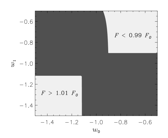
Figure 2: Contourplot of the function $F$. For each value of $(w_{0},w_{1})$, $a_{s}$ and $q$ have been chosen so that $F$ is as close to $F_{0}=1.61$ as possible.

3 Numerical analysis

Since it is not possible to obtain useful limits for all four parameters of our equation of state parametrization in equation 6 and we are primarily interested in exploring evidence for $w\neq-1$ and/or a changing $w$, we employ the following approach: For fixed values of $w_{0}$ and $w_{1}$ we marginalize over the other cosmological parameters. As our framework we choose the minimum standard model with 6 parameters: $\Omega_{m}$, the matter density, the curvature parameter, $\Omega_{b}$, the baryon density, $H_{0}$, the Hubble parameter, and $\tau$, the optical depth to reionization. The normalization of both CMB and LSS spectra are taken to be free and unrelated parameters. The priors we use are given in Table 1.

Table 1: Priors on cosmological parameters used in the likelihood analysis.

• Parameter	Prior	Distribution
  $\Omega=\Omega_{m}+\Omega_{X}$	1	Fixed
  $h$	$0.72\pm 0.08$	Gaussian [74]
  $\Omega_{b}h^{2}$	0.014–0.040	Top hat
  $n_{s}$	0.6–1.4	Top hat
  $\tau$	0–1	Top hat
  $Q$	—	Free
  $b$	—	Free

Likelihoods are calculated from $\chi^{2}$ so that for 1 parameter estimates, 68% confidence regions are determined by $\Delta\chi^{2}=\chi^{2}-\chi_{0}^{2}=1$, and 95% region by $\Delta\chi^{2}=4$. $\chi_{0}^{2}$ is $\chi^{2}$ for the best fit model found. In 2-dimensional plots the 68% and 95% regions are formally defined by $\Delta\chi^{2}=2.30$ and 6.17 respectively. Note that this means that the 68% and 95% contours are not necessarily equivalent to the same confidence level for single parameter estimates.

3.1 Supernova luminosity distances

We perform our likelihood analysis using the “gold” dataset compiled and described in Riess et al [50] consisting of 157 SNIae using a modified version of the SNOC package [51].

3.2 Large Scale Structure (LSS).

At present there are two large galaxy surveys of comparable size, the Sloan Digital Sky Survey (SDSS) [7, 6] and the 2dFGRS (2 degree Field Galaxy Redshift Survey) [5]. Once the SDSS is completed in 2005 it will be significantly larger and more accurate than the 2dFGRS. In the present analysis we use data from SDSS, but the results would be almost identical had we used 2dF data instead. In the data analysis we use only data points on scales larger than $k=0.15h$/Mpc in order to avoid problems with non-linearity.

3.3 Cosmic Microwave Background.

The CMB temperature fluctuations are conveniently described in terms of the spherical harmonics power spectrum $C_{l}^{TT}\equiv\langle|a_{lm}|^{2}\rangle$, where $\frac{\Delta T}{T}(\theta,\phi)=\sum_{lm}a_{lm}Y_{lm}(\theta,\phi)$. Since Thomson scattering polarizes light, there are also power spectra coming from the polarization. The polarization can be divided into a curl-free $(E)$ and a curl $(B)$ component, yielding four independent power spectra: $C_{l}^{TT}$, $C_{l}^{EE}$, $C_{l}^{BB}$, and the $T$-$E$ cross-correlation $C_{l}^{TE}$.

The WMAP experiment has reported data only on $C_{l}^{TT}$ and $C_{l}^{TE}$ as described in Refs. [3, 4, 70, 71, 72]. We have performed our likelihood analysis using the prescription given by the WMAP collaboration [4, 70, 71, 72] which includes the correlation between different $C_{l}$’s. Foreground contamination has already been subtracted from their published data.

4 Results

In Figs. 3-5 we show results of the likelihood analysis. For each $(w_{0},w_{1})$ we have marginalized over all other parameters.

From the figure including CMB and LSS data only it is clear that there is an almost complete parameter degeneracy with the same shape as predicted in Fig. 2, i.e. it follows the degeneracy inherent in the angular distance integral. With the present data there is no way of discriminating between models with strong time variation of $w$, and models with constant $w$.

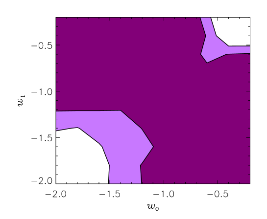
Figure 3: 68% (dark) and 95% (light) likelihood contours for WMAP and SDSS data only.

When only SN data is used there is also an almost perfect degeneracy which comes from the integral $I$ in Eq. (4). Again, there is no means of discriminating between a time varying and a constant $w$.

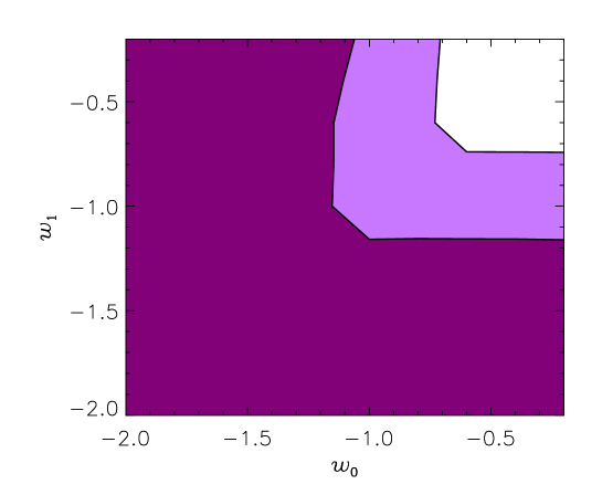
Figure 4: 68% (dark) and 95% (light) likelihood contours for SNI-a data only.

However, once SN, CMB and LSS data are combined this degeneracy is partially broken. From Fig. 5 it is clear that the best fit has $w_{1}>w_{0}$, meaning that $w$ is decreasing with time. The reason that Fig. 5 is not a superposition of Figs. 3 and 4 is that the best fits for the individual subsets of data require different values of $\Omega_{m},a_{s}$ and $q$. In Table 2 we tabulate $\chi^{2}$ for various best fit models, compared with the corresponding best fits for $\Lambda$CDM models $(w_{0}=w_{1}=-1)$. The best fit model to the combined CMB, LSS and SNI-a data has $\chi^{2}=1623.1$, which should be compared to the 1512 degrees of freedom in the fit. The goodness-of-fit (GoF) of this model is 0.0236, indicating that only 2.36% of all randomly generated data sets based on the same underlying cosmological model would produce a worse fit than the one observed. The main cause of this bad fit is the WMAP data, a fact which is well known, and which is presumably due to incomplete foreground removal.

At first sight the models with varying $w$ seem to better fit the data, disfavouring a pure cosmological constant. However, four new parameters are added to the model with time varying $w$. The GoF for the best fit $\Lambda$CDM model is actually 0.0239 ($\chi^{2}=1626.9$ for 1516 degrees of freedom), which is better than for the time-varying $w$ model. Therefore there is no compelling evidence for a time-variation of $w$ in the present data. We elaborate more on this point in section 4.4 where we perform non-parametric rank correlation tests on the SN data.

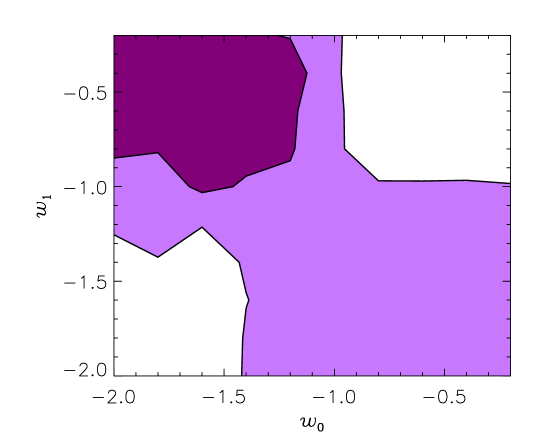
Figure 5: 68% (dark) and 95% (light) likelihood contours for WMAP, SDSS and SNI-a data.

Our best fit model has parameters $w_{1}=-0.4$, $w_{0}=-1.8$, $\Omega_{m}=0.38$, $a_{s}=0.50$, and $q=3.41$. In figure 6 we show $w(z)$ for this model. Evidently the data favour a strongly time-dependent $w$ at present. We note that this result is similar to that of [53]. In this work $w$ is also parameterized as evolving from one asymptotic limit to another, albeit with a different parametrization. Their best fit model is found to have $w_{1}=-0.7$, $w_{0}=-2.0$, using slightly different observational data than is used in the present work.

Table 2: $\chi^{2}$ for the best fit model, compared with $\Lambda$CDM, for different data sets

• Data used	best fit	$\Lambda$CDM
  CMB+LSS	1446.7	1447.3
  SNI-a	173.8	177.1
  CMB+LSS+SNI-a	1623.1	1626.9

Figure 6: Evolution of $w$ in the best-fit model found.

4.1 A constant equation of state

The simplest possibility for dark energy is that $w$ is constant. Constraints on this type of model can be found by setting $w_{0}=w_{1}$, effectively taking line sections through the $(w_{0},w_{1})$ likelihood plots. The resulting 1D $\chi^{2}$ curves can be seen in figure 7. From the combination of all available data we find that $-1.34\leq w\leq-0.79$, in good agreement with other recent analyses [49, 50].

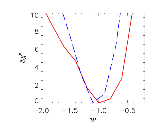
Figure 7: Likelihood functions for the case of $w_{0}=w_{1}$. The full (red) line is for WMAP+SDSS, and the dashed (blue) for WMAP+SDSS+SNI-a data.

4.2 Parametrization in terms of $w(z=0)$ and $dw/dz(z=0)$

In fact our parametrization can easily be reduced to a model where the fit is done for $w(z=0)\equiv w_{*}$ and $dw/dz(z=0)\equiv w_{*}^{\prime}$.

To do a one dimensional fit over $w_{*}$, one simply rewrites $w_{1}$ as

$$w_{1}=\frac{w_{*}a_{s}^{q}w_{0}}{w_{0}(1+a_{s}^{q})-w_{*}}$$ (9)

When the likelihood analysis is done, $w_{0}$ is a free parameter and $w_{1}$ given by the relationship above. The result of this exercise is shown in Fig. 8. From this it can be seen that the best fit is at $w_{*}=-1.43$ as described above, and that $w_{*}=-1$ is disfavoured at about $2\sigma$, which is also in accordance with our previous finding. The $1\sigma$ allowed interval is $w_{*}=-1.43^{+0.16}_{-0.38}$. While the best fit value is very close to what is obtained by Alam et al. [58, 59], and also by Riess et al., the error bars are different from those of Riess et al. The reason is that we add other observational data which shift the best fit value, and also that differences between our parametrization and the Taylor series used in other analyses increase when moving away from the best fit values. Basically our parametrization has more freedom to fit data because there are additional free parameters. This in turn means that the one-parameter error bars increase.

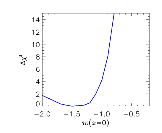
Figure 8: $\chi^{2}$ as a function of the present day value of $w$ for the WMAP+SDSS+SNI-a data.

Equally, it is possible to do a parametrization in terms of $w_{*}^{\prime}$ instead in the following way. First, the derivative of $w$ with respect to $a$ is

$$w_{*}^{\prime}=-\left.\frac{dw}{da}\right|_{z=0}=\frac{w_{0}w_{1}qa_{s}^{q}(w_{1}-w_{0})}{(w_{1}+a_{s}^{q}w_{0})^{2}}.$$ (10)

We now introduce a new variable $x=a_{s}^{q}$. By doing this, we can solve the above equation for $q$

$$q=w_{*}^{\prime}\frac{(w_{1}+xw_{0})^{2}}{w_{0}w_{1}x(w_{0}-w_{1})}.$$ (11)

In the likelihood analysis, the free parameters are then $w_{0},w_{1}$ and x, whereas $q$ is given by the above relation. The result of this analysis is shown in Fig. 9

Formally, the 1$\sigma$ allowed interval is $w_{*}^{\prime}=1.0^{+1.0}_{-0.8}$. However, as is evident from the figure the likelihood is far from Gaussian, and no useful constraints can be placed at the 2$\sigma$ level.

4.3 Comparison with analyses based on Taylor series expansions

Tentative evidence for evolution of $w$ has been found in several other analyses of supernova data. Most analyses of SN data use a Taylor series expansion of $w$ around $z=0$ because no high redshift data is used. One recent example is the work of Alam et al. [58, 59] where the parametrization

$$\rho_{DE}=A_{0}+A_{1}(1+z)+A_{2}(1+z)^{2}$$ (12)

is used. This can be translated into a relation for $w$

$$w(z)=-1+\frac{1+z}{3}\frac{A_{1}+2A_{2}(1+z)}{A_{0}+A_{1}(1+z)+A_{2}(1+z)^{2}},$$ (13)

where $A_{0}=1-\Omega_{m}-A_{1}-A_{2}$.

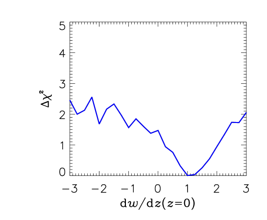
Figure 9: $\chi^{2}$ as a function of the present day value of $dw/dz$ for the combined WMAP+SDSS+SNI-a data.

The best fit found in that work is $\Omega_{m}=0.3$, $A_{1}=-4.36$, $A_{2}=1.83$ (slightly better fits are found for higher $\Omega_{m}$, but the corresponding $A_{1}$ and $A_{2}$ are not tabulated). This leads to

$$w|_{z=0}=-1.33\,\,\,\,\,\, \,\,\,\,\,\,\left.\frac{dw}{dz}\right|_{z=0}=1.07$$ (14)

Our results cannot be compared on global scale because the Taylor series expansion quickly breaks down (in fact it cannot generally be expected to be valid even at $z\sim 1$). The only direct comparison available is in terms of the present $w$ and its derivative.

As described above, we find that the best fit model has

$$w|_{z=0}=-1.4\,\,\,\,\,\, \,\,\,\,\,\,\left.\frac{dw}{dz}\right|_{z=0}=1.0$$ (15)

which is almost identical to what is found by Alam et al.

As discussed previously the reason that $dw/dz\neq 0$ is a better fit than a constant $w$ is exactly the supernova data, and therefore our results can be expected to be very similar in the one limit where they can be directly compared.

4.4 SNIa data rank correlation test

Since the SNIa data are best fit by a changing $w$ and there are different opinions about the significance of the effect and the dependence on the specific dark energy model, we have also investigated the need for additional parameters in the luminosity distance relation by studying the correlation between the observed magnitude and the redshift after subtracting the best fit cosmology magnitudes. This can be done in an non-parametric manner using the Spearman or Kendall rank correlation tests. The two-sided significance level, $p$ (ranging from 0 to 1), of the deviation from zero correlation indicates whether the model is capable of representing the complexity of the actual data or not. A small value of $p$ indicates a significant correlation or anticorrelation. For an Einstein-de Sitter universe, we get $p\,\hbox to0.0pt{\lower 3.7pt\hbox{$\mathchar 0\relax\sim$}\hss}\raise 1.0pt\hbox{$<$}\,10^{-19}$, indicating – as expected – that this simple model is not able to mimic the observed magnitudes over a wide redshift range. Fitting $\Omega_{m}$ for a zero cosmological constant universe, we get $p\sim 0.17-0.19$ (for $\Omega_{m}=0$), showing a better but still unsatisfactory fit. Including a cosmological constant with or without a flat universe assumption removes any evidence of correlation (see table 3) and disfavouring the need for more complexity in the dark energy model. We have also simulated a sample 100 SNIa data sets with the same number and redshift distribution of SNe as the Riess gold sample assuming a cosmological constant flat universe with $\Omega_{m}=0.3$ and a dispersion in SN magnitudes of 0.3 mag. Subtracting the best fit cosmological constant flat universe and performing the rank correlation tests on each simulation yields

$$\Omega_{m} = 0.31\pm 0.05$$

$$p_{S} = 0.47\pm 0.29$$

$$p_{K} = 0.47\pm 0.30.$$ (16)

Comparing with the results in table 3 it is clear that the real data actually have a smaller deviation from zero correlation than is expected for a cosmological constant universe, thus weakening the case for a evolving $w$.

This result is completely consistent with the fact that the Goodness-of-Fit for the combined CMB, LSS, and SNI-a analysis is slightly worse for the time-varying $w$ models than for pure $\Lambda$CDM models.

Table 3: Result from likelihood analysis and correlation test. $p_{S}$ and $p_{K}$ are the two-sided significance level (ranging from 0 to 1) of the deviation from zero for the Spearman and Kendall rank correlation tests. A small value of $p$ indicates a significant correlation or anticorrelation.

• Cosmology	Best fit parameters	$p_{S}$	$p_{K}$
  Einstein-de Sitter	—	$10^{-19}$	0
  Matter dominated	$\Omega_{m}=0$	0.20	0.17
  $\Omega_{m}+\Omega_{\Lambda}=1$	$\Omega_{m}=0.31$	0.88	0.86
  $\Omega_{m}$ and $\Omega_{\Lambda}$	$\Omega_{m}=0.46,\,\Omega_{\Lambda}=0.98$	0.88	0.86
  Flat with const. $w$	$\Omega_{m}=0.49,\,w=-2.4$	0.88	0.89
  Flat with linear $w$	$\Omega_{m}=0.48,w\,_{*}=-2.5,w\,_{*}^{\prime}=2.0$	0.98	0.98

4.5 Extending the parametrization

The parametrization used in the present analysis already involves more parameters than can be unambiguously fitted with present data. Nevertheless it it still interesting to see how the parametrization naturally extends to a larger number of parameters.

If we still use the assumption that the transition is between two asymptotic values of $w$, the next natural parameter to add is a skewness in the transition profile. This can for instance be incorporated with the parametrization

$$w(a)=w_{0}w_{1}\frac{a^{q+(a/a_{s})^{r}-1}+a_{s}^{q}}{a^{q+(a/a_{s})^{r}-1}w_{1}+a_{s}^{q}w_{0}},$$ (17)

where $r$ is a new parameter. For negative $r$ the transition is more rapid at early times, whereas for positive $r$ it is more rapid at late times. In fig. 10 we show the effect of adding $r$ as a new parameter.

Figure 10: $w(a/a_{s})$ for different values of $r$. Other parameters have been fixed to $w_{0}=-1.5$, $w_{1}=-0.5$, $q=3$. The full line is for $r=0$, the dashed for $r=2$ and the dotted for $r=-2$.

Another possibility is that there are several transitions in $w$ during the evolution of the universe. This is also simple to incorporate. The initial transition is described by

$$w_{i}(a)=w_{0}w_{1}\frac{a^{q}+a_{s}^{q}}{a^{q}w_{1}+a_{s}^{q}w_{0}}.$$ (18)

To add a second transition, simply take

$$w(a)=w_{i}(a)w_{2}\frac{a^{r}+a_{s2}^{r}}{a^{r}w_{2}+a_{s2}^{r}w_{i}(a)},$$ (19)

where $a_{s2}$ is the scale factor at the transition $w_{0}\to w_{1}$, and $r$ describes how rapid the transition is. In figure 11 we show a model which has the second transition at $a_{s2}=20a_{s}$, $q=5$, $r=2$, $w_{1}=-0.5$, $w_{0}=-1.5$, and $w_{2}=-1.7$. By this iterative procedure, more and more steps can be added to the parametrization.

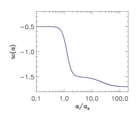
Figure 11: $w(a/a_{s})$ for a model with two transitions.

Finally, we note that our parametrization is well-behaved only if $w<0$, even though $w$ can be arbitrarily close to 0. If there is a transition from $w>0$ to $w<0$ there is a singularity in $w$. However, this can easily be cured by taking instead $w(a)=(a^{q}w_{0}+a_{s}^{q}w_{1})/(a^{q}+a_{s}^{q})$.

5 Conclusion

We have analysed present cosmological data, using an extension of the current minimal cosmological model to allow for time-variation in the dark energy equation of state, $w$.

The result of the likelihood analysis is that the data favour a $w$ which is currently undergoing a rapid transition towards a more negative value. In our parametrization where $w$ varies between two asymptotic values, the best fit is $w(z\to\infty)=-0.4$, and $w(1+z\to 0)=-1.8$. This result agrees well with other analyses using different parametrizations.

The 1$\sigma$ allowed interval for the present value of $w$ is $w(z=0)=-1.43^{+0.16}_{-0.38}$ and for its derivative $dw/dz(z=0)=1.0^{+1.0}_{-0.8}$.

Even though pure $\Lambda$CDM models have higher $\chi^{2}$ values, they also have more fitting parameters. When the Goodness-of-Fit is calculated for both types of models, the best fit $\Lambda$CDM model has GoF = 0.0239, whereas the time-varying $w$ model has GoF = 0.0236. This indicates that there is no real evidence for a time variation of $w$ in the present data. This finding is corroborated by rank correlation tests on the SNI-a data. From Spearman and Kendalls tests we again find that time-varying $w$ models do not produce a statistically significant improvement in the fit to data.

Finally we have discussed in some detail how to extend our parametrization of $w$ to allow for a more refined description once better data becomes available.

References

References

- [1] A. G. Riess et al. [Supernova Search Team Collaboration], Astron. J. 116, 1009 (1998) [arXiv:astro-ph/9805201].
- [2] S. Perlmutter et al. [Supernova Cosmology Project Collaboration], “Measurements of Omega and Lambda from 42 high-redshift supernovae,” Astrophys. J. 517 (1999) 565 [astro-ph/9812133].
- [3] C. L. Bennett et al., “First year Wilkinson Microwave Anisotropy Probe (WMAP) observations: Preliminary maps and basic results,” Astrophys. J. Suppl. 148 (2003) 1 [astro-ph/0302207].
- [4] D. N. Spergel et al., Astrophys. J. Suppl. 148 (2003) 175 [astro-ph/0302209].
- [5] M. Colless et al., astro-ph/0306581.
- [6] M. Tegmark et al. [SDSS Collaboration], astro-ph/0310723.
- [7] M. Tegmark et al. [SDSS Collaboration], astro-ph/0310725.
- [8] C. Wetterich, Nucl. Phys. B 302, 668 (1988).
- [9] P. J. E. Peebles and B. Ratra, Astrophys. J. 325, L17 (1988).
- [10] B. Ratra and P. J. E. Peebles, Phys. Rev. D 37, 3406 (1988).
- [11] D. F. Mota and C. van de Bruck, arXiv:astro-ph/0401504.
- [12] I. Zlatev, L. M. Wang and P. J. Steinhardt, Phys. Rev. Lett. 82, 896 (1999) [arXiv:astro-ph/9807002].
- [13] L. M. Wang, R. R. Caldwell, J. P. Ostriker and P. J. Steinhardt, Astrophys. J. 530, 17 (2000) [arXiv:astro-ph/9901388].
- [14] P. J. Steinhardt, L. M. Wang and I. Zlatev, Phys. Rev. D 59, 123504 (1999) [arXiv:astro-ph/9812313].
- [15] F. Perrotta, C. Baccigalupi and S. Matarrese, Phys. Rev. D 61, 023507 (2000) [arXiv:astro-ph/9906066].
- [16] L. Amendola, Phys. Rev. D 62, 043511 (2000) [arXiv:astro-ph/9908023].
- [17] T. Barreiro, E. J. Copeland and N. J. Nunes, Phys. Rev. D 61, 127301 (2000) [arXiv:astro-ph/9910214].
- [18] O. Bertolami and P. J. Martins, Phys. Rev. D 61, 064007 (2000) [arXiv:gr-qc/9910056].
- [19] C. Baccigalupi, A. Balbi, S. Matarrese, F. Perrotta and N. Vittorio, Phys. Rev. D 65, 063520 (2002) [arXiv:astro-ph/0109097].
- [20] R. R. Caldwell, M. Doran, C. M. Mueller, G. Schaefer and C. Wetterich, Astrophys. J. 591, L75 (2003) [arXiv:astro-ph/0302505].
- [21] C. Armendariz-Picon, T. Damour and V. Mukhanov, Phys. Lett. B 458, 209 (1999) [arXiv:hep-th/9904075].
- [22] T. Chiba, T. Okabe and M. Yamaguchi, Phys. Rev. D 62, 023511 (2000) [arXiv:astro-ph/9912463].
- [23] C. Armendariz-Picon, V. Mukhanov and P. J. Steinhardt, Phys. Rev. D 63, 103510 (2001) [arXiv:astro-ph/0006373].
- [24] L. P. Chimento, Phys. Rev. D 69, 123517 (2004) [arXiv:astro-ph/0311613].
- [25] P. F. Gonzalez-Diaz, Phys. Lett. B 586, 1 (2004) [arXiv:astro-ph/0312579].
- [26] R. J. Scherrer, arXiv:astro-ph/0402316.
- [27] J. M. Aguirregabiria, L. P. Chimento and R. Lazkoz, arXiv:astro-ph/0403157.
- [28] R. R. Caldwell, Phys. Lett. B 545, 23 (2002) [arXiv:astro-ph/9908168].
- [29] S. M. Carroll, M. Hoffman and M. Trodden, Phys. Rev. D 68, 023509 (2003) [arXiv:astro-ph/0301273].
- [30] G. W. Gibbons, arXiv:hep-th/0302199.
- [31] R. R. Caldwell, M. Kamionkowski and N. N. Weinberg, Phys. Rev. Lett. 91, 071301 (2003) [arXiv:astro-ph/0302506].
- [32] A. E. Schulz and M. J. White, Phys. Rev. D 64, 043514 (2001) [arXiv:astro-ph/0104112].
- [33] S. Nojiri and S. D. Odintsov, Phys. Lett. B 562, 147 (2003) [arXiv:hep-th/0303117].
- [34] P. Singh, M. Sami and N. Dadhich, Phys. Rev. D 68, 023522 (2003) [arXiv:hep-th/0305110].
- [35] M. P. Dabrowski, T. Stachowiak and M. Szydlowski, Phys. Rev. D 68, 103519 (2003) [arXiv:hep-th/0307128].
- [36] J. G. Hao and X. z. Li, arXiv:astro-ph/0309746.
- [37] H. Stefancic, Phys. Lett. B 586, 5 (2004) [arXiv:astro-ph/0310904].
- [38] J. M. Cline, S. y. Jeon and G. D. Moore, arXiv:hep-ph/0311312.
- [39] M. G. Brown, K. Freese and W. H. Kinney, arXiv:astro-ph/0405353.
- [40] V. K. Onemli and R. P. Woodard, arXiv:gr-qc/0406098.
- [41] V. K. Onemli and R. P. Woodard, Class. Quant. Grav. 19, 4607 (2002) [arXiv:gr-qc/0204065].
- [42] A. Vikman, arXiv:astro-ph/0407107.
- [43] C. Deffayet, G. R. Dvali and G. Gabadadze, Phys. Rev. D 65, 044023 (2002) [arXiv:astro-ph/0105068].
- [44] G. Dvali and M. S. Turner, arXiv:astro-ph/0301510.
- [45] P. S. Corasaniti and E. J. Copeland, Phys. Rev. D 65, 043004 (2002) [arXiv:astro-ph/0107378].
- [46] R. Bean and A. Melchiorri, Phys. Rev. D 65, 041302 (2002) [arXiv:astro-ph/0110472].
- [47] S. Hannestad and E. Mortsell, Phys. Rev. D 66, 063508 (2002) [arXiv:astro-ph/0205096].
- [48] A. Melchiorri, L. Mersini, C. J. Odman and M. Trodden, Phys. Rev. D 68, 043509 (2003) [arXiv:astro-ph/0211522].
- [49] Knop, R. A., et al. 2003, ApJ, 598, 102
- [50] Riess, A. G., et al. 2004, ApJ, 607, 665
- [51] Goobar, A., Mörtsell, E., Amanullah, R., Goliath, M., Bergström, L. and Dahlén, T., 2002, A&A, 392, 757 [arXiv:astro-ph/0206409]. Code available at http://www.physto.se/ariel/snoc/
- [52] Maor I., Brustein R., Steinhardt P. J., 2001, PhRvL, 86, 6; Maor I., Brustein R., Steinhardt P. J., 2001, PhRvL, 87, 049901
- [53] Corasaniti, P.S., Kunz, M., Parkinson, D., Copeland, E.J., Bassett, B.A., astro-ph/0406608
- [54] Gong, Y., astro-ph/0405446
- [55] Gong, Y., astro-ph/0401207
- [56] S. Nesseris and L. Perivolaropoulos, arXiv:astro-ph/0401556.
- [57] B. Feng, X. L. Wang and X. M. Zhang, arXiv:astro-ph/0404224.
- [58] Alam U., Sahni V., Starobinsky A. A., astro-ph/0406672
- [59] Alam U., Sahni V., Starobinsky A. A., 2004, JCAP, 6, 8
- [60] Corasaniti, P.-S., Copeland, E.-J., astro-ph/0205544
- [61] H. K. Jassal, J. S. Bagla and T. Padmanabhan, arXiv:astro-ph/0404378.
- [62] T. R. Choudhury and T. Padmanabhan, arXiv:astro-ph/0311622.
- [63] Huterer, D., & Cooray, A., astro-ph/0404062
- [64] Daly R. A., Djorgovski S. G., 2003, ApJ, 597, 9
- [65] Wang, Y., & Tegmark, M., astro-ph/0403292
- [66] Wang, Y., & Freese, K., astro-ph/0402208
- [67] Wang Y., Mukherjee P., 2004, ApJ, 606, 654
- [68] Jonsson, J., Goobar, A., Amanullah, R., & Bergstrom, L., astro-ph/0404468
- [69] Linder E. V., 2003, PhRvL, 90, 091301
- [70] L. Verde et al., Astrophys. J. Suppl. 148 (2003) 195 [astro-ph/0302218].
- [71] A. Kogut et al., Astrophys. J. Suppl. 148 (2003) 161 [astro-ph/0302213].
- [72] G. Hinshaw et al., Astrophys. J. Suppl. 148 (2003) 135 [astro-ph/0302217].
- [73] U. Seljak and M. Zaldarriaga, Astrophys. J. 469 (1996) 437 [astro-ph/9603033]. See also the CMBFAST website at http://cosmo.nyu.edu/matiasz/CMBFAST/cmbfast.html
- [74] W. L. Freedman et al., Astrophys. J. Lett. 553, 47 (2001).