A CFH12k Lensing Survey of X-ray Luminous Galaxy Clusters

We describe the weak lensing methodology we have applied to multi-colour CFH12k imaging of a homogeneously-selected sample of luminous X-ray clusters at $z\sim 0.2$. The aim of our survey is to understand the variation in cluster structure and dark matter profile within rich clusters. The method we describe converts a fully reduced CFH12k image into constraints on the cluster mass distribution in two steps: (1) determination of the “true” shape of faint (lensed) galaxies, including object detection, point spread function (PSF) determination, galaxy shape measurement with errors; (2) conversion of the faint galaxy catalogue into reliable mass constraints using a range of 1D and 2D lensing techniques. Mass estimates are derived independently from each of the three images taken in separate filters to quantify the systematic uncertainties. Finally, we compare the cluster mass model to the light distribution of cluster members as derived from our imaging data. To illustrate the method, we apply it to the well-studied cluster Abell 1689 ($z=0.184$). In this cluster, we detect the gravitational shear signal out to $\sim 3$ Mpc at $>$3-$\sigma$ significance. The two-dimensional mass reconstruction has a $\sim$10-$\sigma$ significance peak centered on the brightest cluster galaxy. The weak lensing profile is well fitted by a NFW mass profile with $M_{200}=14.1^{+6.3}_{-4.7}\times 10^{14}\,M_{\sun}$, and $c=3.5^{+0.5}_{-0.3}$ ($\chi^{2}=0.33$), or by a power law profile with $q=0.75\pm 0.07$ and $\theta_{\rm E}=14\aas@@fstack{\prime\prime}6\pm 0\aas@@fstack{\prime\prime}3$ ($\chi^{2}=0.64$). The mass-to-light ratio is found to be almost constant with radius with a mean value of $M/L_{R}=150\,h\,(M/L)_{\sun}$. We compare these results to other weak lensing analyses of Abell 1689 from the literature and find good agreements in terms of the shear measurement as well as the final mass estimate.

1 Introduction

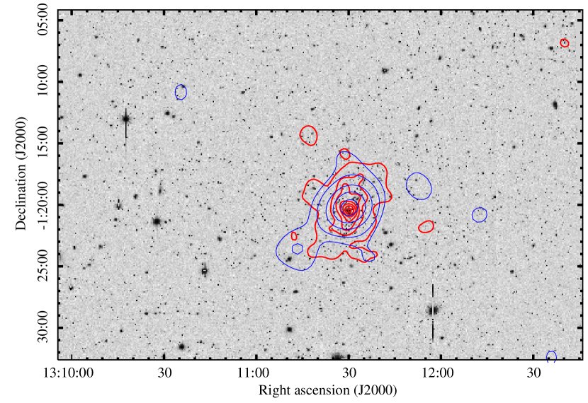
Figure 1: The full $42\arcmin\times 28\arcmin$ CFH12k R-band image of Abell 1689. The thick contours represent the number density of bright galaxies selected in the R-band: the first contour corresponds to 5 objects per square arcmin, increased by steps of 5 units. The maximal density is 36.5 galaxies ${\rm arcmin}^{-2}$ in the cluster center. The thin contours represent the mass density reconstruction with LensEnt2 and an ICF of 180″ (see Sect. 4.2 for more details). Contour levels are respectively 2, 3, 5, 7 and $9\sigma$, while the peak value corresponds to a mass density of $1100\ {\rm h}_{70}\ M_{\sun}.{\rm pc}^{-2}$. North is to the top, East to the right.

Clusters of galaxies are the most massive collapsed structures in the Universe. They are located at the nodes of the filamentary cosmic web, as mapped by the SDSS and 2dF redshift surveys. These massive systems are the focus of both theoretical (e.g.  Eke et al. 1996; Bahcall et al. 1997; Viana & Liddle 1998) and observational studies. The aim is to better understand cluster formation and evolution and thus it is important to quantify their physical properties as precisely as possible (e.g. mass distribution, mass density profile, importance of substructure, etc.). Different techniques such as galaxy dynamics, X-ray emission, the Sunyaev-Zeldovich effect or gravitational lensing, are available to probe the physical properties of clusters. Gravitational lensing is a particularly attractive method as it is directly sensitive to the total mass distribution irrespective of its physical state (see the review by Mellier 1999).

Although the study of a single cluster can be instructive, we need to study homogeneous samples of massive clusters in order to better understand cluster physics, test theoretical predictions and to constrain the cosmological and physical parameters governing the growth of structure in the Universe. Indeed, clusters are expected to show some variation in their properties, in particular in the amount of substructure and their merger history, which can be directly probed by measuring their mass distribution. Thus to obtain a representative view of the properties of clusters, a fair and statistically-reliable sample of cluster needs to be studied.

In order to obtain a better understanding of the mass distributions on small and large scales in clusters, we have selected a sample of 11 X-ray luminous clusters (Czoske et al. 2003; Smith et al. 2005) identified in the XBACs sample (X-ray Brightest Abell-type Clusters: Ebeling et al. 1996). All these clusters have X-ray luminosities of $L_{\rm X}\geq 8\times 10^{44}\,\mathrm{erg\,s^{-1}}$ in the 0.1–2.4 keV band, and all lie in a narrow redshift slice at $z\sim 0.2$ (from $z_{\rm A2218}=0.171$ to $z_{\rm A1835}=0.253$). As XBACS is restricted to Abell clusters (Abell et al. 1989), it is X-ray flux-limited but not truly X-ray selected. However, a comparison with the X-ray selected ROSAT Brightest Cluster Sample (BCS: Ebeling et al. 1998, 2000) shows that $\sim 75\%$ of the BCS clusters in the redshift and X-ray luminosity range of our sample are in fact Abell clusters. Hence, our XBACs sample is, in all practical aspects, indistinguishable from an X-ray selected sample.

Using the CFH12k wide field camera (Cuillandre et al. 2000) mounted at the Canada-France-Hawaii Telescope (CFHT), we imaged all 11 clusters in our sample in the B, R and I bands. In the present paper we present the weak lensing methodology we have applied to analyse these images, using our observations of Abell 1689 as a test case.

The first step of any weak lensing work is to correct the observed galaxy ellipticities for any observational smearing: circularization or anisotropy due to the point spread function (PSF). The classical approach to do this is the so-called KSB method (Kaiser et al. 1995), implemented in the imcat software (see also Luppino & Kaiser 1997; Rhodes et al. 2000; Kaiser 2000). The basic idea is to relate the “true” ellipticity of the background sources to the observed ellipticity through polarizability tensors, which include the smearing effect of the PSF, possibly with anisotropic components. In practice these can be computed through the combination of the second order moments of the light distribution of the galaxies and the PSF itself. However, in this paper we will use an inverse approach through a maximum likelihood or Bayesian estimate of the source galaxy shape convolved by the local PSF (this method was first proposed by Kuijken 1999). Both the galaxy shape and the local PSF are modeled in terms of sums of elliptical Gaussians. This approach is implemented in the software Im2Shape which has been developed by Bridle et al. (2001). The main advantage of Im2Shape is that it provides estimates of the uncertainties of the recovered parameters of the sources and these uncertainties can then be included in the mass inversion.

In the weak lensing limit, the ellipticities of background galaxies give an unbiased estimate of the shear field induced by the gravitational potential of the foreground cluster. The estimate is inherently noisy due to the shape measurement errors and the intrinsic ellipticities of the galaxies. Several methods have been proposed to reconstruct the mass density field (or the potential) of the foreground structure from the measured shear field. Non-parametric methods are usually best to produce a mass-map, necessary to identify mass peaks. They can also be used to estimate the cluster mass profile by means of the aperture mass densitometry method (Fahlman et al. 1994; Schneider 1996). On the other hand parametric methods are best to constrain the cluster mass profile and total mass by fitting a radial shear profile to the galaxy ellipticities.

To illustrate the various methods and techniques used, we apply our procedure to one particulary well-studied cluster from our sample, Abell 1689. Abell 1689 at $z=0.184$ is one of the richest clusters ($R=4$) in the Abell catalog. Abell 1689 is a powerful cluster lens and has been studied by various groups using different lensing techniques (Tyson et al. 1990; Tyson & Fischer 1995; Taylor et al. 1998; Clowe & Schneider 2001; King et al. 2002). It has also been studied in X-rays using Chandra (Xue & Wu 2002) and XMM-Newton (Andersson & Madejski 2004). The central structure of this cluster is complex: from the redshift distribution of 66 cluster members Girardi et al. (1997) find evidence for a superposition of several groups along the line of sight to the cluster center which explains the extraordinarily high velocity dispersion of $2355^{+238}_{-183}\,\mathrm{km\,s^{-1}}$. Czoske (2004) has recently obtained a new large dataset of more than 500 cluster galaxy redshifts in this cluster, which will help elucidate the galaxy distribution Abell 1689. Preliminary analysis of these data shows that the large scale distribution of galaxies in and around Abell 1689 is in fact rather smooth and that significant substructure seems confined to the very center of the cluster. Thus, even though the cluster has clear substructure, it may still be reasonable to model the large-scale mass distribution of the cluster with simple models, such as the “universal” mass profile proposed by Navarro et al. (1997) (NFW).

This paper is organized as follows: §2 briefly presents the observations of Abell 1689 used in this paper and gives a summary of the data reduction procedure and the conversion of the reduced data into catalogues that can be used in the weak lensing analysis. In §3 we present the measurement of galaxy shapes and correction for PSF anisotropy using Im2Shape. In §4 we convert the galaxy shape measurements into two-dimensional shear maps and radial shear profiles. §5 explains how we model the lensing data using both 1D and 2D techniques. In §6 we compare the projected mass to the light distribution in the cluster. Finally in §7 we discuss our method and results. In a separate paper (Bardeau et al. 2005, in prep.) we will present a more extensive analysis of the mass distribution in Abell 1689 combining weak and strong lensing mass measurements.

We assume $H_{0}=70\,\mathrm{km\,s^{-1}\,Mpc^{-1}}$, $\Omega_{\rm m}=0.3$, $\Omega_{\Lambda}=0.7$. At $z=0.18$, $1\arcsec$ corresponds to $3.09\,\mathrm{kpc}$ (and $1\arcmin$ to $185\,\mathrm{kpc}$).

2 Observations and Cataloging

We observed Abell 1689 with the CFH12k camera through the B, R and I filters (Fig. 1 shows the R-band image) between 30 May and 2 June 2000. The camera consists of 12 CCD chips of $2\mathrm{k}\times 4\mathrm{k}$ pixels with a total field of view of $42\arcmin\times 28\arcmin$ at a pixel scale of $0\aas@@fstack{\prime\prime}205$. The log of the observations of Abell 1689 ($\alpha_{\rm J2000}\!=\!13^{\rm h}11^{\rm m}30^{\rm s}$, $\delta_{\rm J2000}\!=\!-01\degr 20\arcmin 28\arcsec$) is summarized in the first part of Table 1.

Table 1: Observing log for Abell 1689. We indicate the number of detections in each filter (B, R or I), their number density (expressed in arcmin^-2, in parenthesis), and the magnitude cuts for galaxy classification. Estimated average redshifts $\bar{z}$ and $\bar{\beta}=\langle D_{\rm ls}/D_{\rm s}\rangle$, with their standard deviations, are given for the faint galaxy catalogues (see §3.3 for details).

Filter	B			R			I
Date of observation	May 30/June 2 2000			May 30/June 2 2000			May 30/June 2 2000
Number of exposures	4			5			5
Exposure time (sec)	3600			3000			3000
Seeing	$0.91\arcsec$			$0.85\arcsec$			$0.88\arcsec$
Completeness mag	24.9			24.3			22.6
PSF anisotropy	$0.032\pm 0.012$			$0.071\pm 0.019$			$0.064\pm 0.028$
Number of Detections		34669	(28.6)		41067	(33.9)		28805	(23.7)
Stars		2223	(1.8)		3488	(2.9)		2397	(2.0)
Galaxies		25823	(21.3)		30189	(24.9)		21145	(17.4)
Others		6623	(5.5)		7390	(6.1)		5263	(4.3)
Bright galaxies	B$<$22.0	1171	(1.0)	R$<$21.1	2166	(1.8)	I$<$19.3	950	(0.8)
Faint galaxies	22.5$<$B$<$25.4	20186	(16.7)	21.6$<$R$<$24.7	22794	(18.8)	19.8$<$I$<$23.3	14382	(11.8)
Other galaxies	22.0$<$B$<$22.5			21.1$<$R$<$21.6			19.3$<$I$<$19.8
	or B$>$25.4	4466	(3.7)	or R$>$24.7	5229	(4.3)	or I$>$23.3	5813	(4.8)
Faint galaxies $\bar{z}$	1.02$\pm 0.42$			1.06$\pm 0.42$			0.82$\pm 0.35$
Faint galaxies $\bar{\beta}$	0.70$\pm 0.08$			0.69$\pm 0.08$			0.65$\pm 0.07$

2.1 Data reduction

For a detailed description of the data reduction see Czoske (2002). Here we just give a brief outline. Pre-reduction of the CFH12k data was done in a standard way using the iraf package mscred (Valdes 1998) for bias subtraction and flat-fielding using twilight sky images.

Fringing in the I band images was removed by subtracting a correction image constructed from eight science images from different fields taken during the same night, after masking any objects detected in the images. The appropriate scaling for the fringe correction was determined interactively.

Weak lensing applications demand precise measurements of the shapes of faint galaxies and therefore precise relative astrometric alignment of the individual dithered exposures of the field ($\sim 6\arcsec$ in our case). A transformation is needed between each chip of the input image and a common astrometric output grid which has to account for the position of the chip in the focal plane, rotation, variations in the height (and possibly tilt) of the chip surface with respect to the focal plane, as well as any optical distortion induced by the telescope and camera optics. Fourth order polynomials were found to be sufficient to model these effects. The method that we have developed follows the approach described by Kaiser et al. (1999).

We use Digital Sky Survey (DSS) images to define the external reference frame for observations, but then minimize the RMS dispersion of the transformed object coordinates from all the exposures rather than the deviations between the transformed object coordinates from the corresponding DSS coordinates for each individual exposure. This approach ensures optimal relative alignment of the transformed exposures. The resulting RMS dispersion of the transformed coordinates is of order $0\aas@@fstack{\prime\prime}01$, corresponding to 0.05 of a CFH12k pixel, for usually $\gg\!100$ objects per chip.

The input images are resampled onto the output grid with pixel size $0\aas@@fstack{\prime\prime}205$ (the median effective pixel scale of the CFH12k camera) using the software swarp (Version 1.21). Pixel interpolation uses the lanczos3 kernel which preserves object counts, without introducing strong artifacts around image discontinuities (Bertin 2001). Fields with a large number of exposures ($\geq 10$) were averaged after rejecting outliers, those with fewer exposures median combined.

The images were photometrically calibrated on fields of standard stars taken from the list of Landolt (1992) with additional photometry by Stetson (2000). Atmospheric extinction was determined from sequences of science images spanning a sufficient range in airmass to allow accurate determination of the extinction coefficient.

2.2 Object detection

With the reduced and calibrated images in hand, the weak shear information must be extracted from the photometric catalogues. The analysis of the images involves a number of steps that we describe in detail below. These various steps are controlled in (as much as possible) an automatic way using different perl scripts which allow a simple and easy handling of catalogues and can easily call external programmes.

In the present paper we first treat the images taken in the three filters B, R and I independently. Differences between the results obtained from the three datasets are expected due to a number of effects. Different seeing in the images affects the accuracy of the measurement of galaxy shapes and hence the accuracy of the derived shear fields. Different photometric depths of the images will change the number density of faint background galaxies and thus again the accuracy of the shear measurements. Finally, the images sample different wavebands of the observed galaxies, which has an effect on the contrast between cluster and background galaxies if these are selected based on magnitude alone. This independent approach allows us to assess the uncertainties introduced by the listed effects. Of course it is desirable to eventually combine the information present in the three images in an optimal way so as to arrive at definitive measurements of the physical properties of the cluster. A first attempt at this combination is implemented here but will be discussed in more detail in a forthcoming paper.

The first step is to construct a master photometric catalogue of each individual image. For this purpose and to automate the procedure as much as possible we have used sextractor (Bertin & Arnouts 1996) in a two-pass mode. A first run is made to detect bright objects, with a detection level of $5\sigma$ above the background. The average size (full width at half maximum, FWHM) of the point spread function (PSF) is then easily determined from the sizes of stars. The saturation level of the image is also determined in this run. These parameters are then fed into a second sextractor run with a lower detection level ($1.5\,\sigma$ with a minimum size of 5 connected pixels above the threshold). This second output catalogue corresponds to the working catalogue. The total number of objects detected in each image is given in Table 1. The photometry was computed using the mag_auto method of sextractor.

2.3 Star catalogue

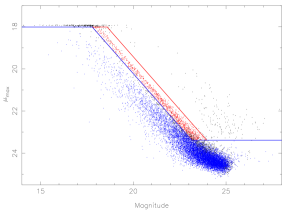
a)

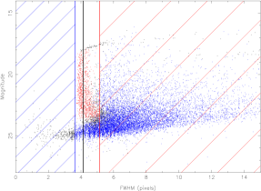
      b)

Figure 2: a) Magnitude-$\mu_{\rm max}$ diagram for all objects detected by sextractor in the Abell 1689 R-band image. The points inside the parallelogram correspond to stars, the points below to galaxies. Points on the upper left correspond to cosmic rays, defects and saturated objects. b) FWHM-magnitude diagram for all the objects detected by sextractor in the Abell 1689 R-band image. The vertical black line indicates the average seeing value (4.15 pixels for the Abell 1689 R-band image). Stars are excluded from the right hatched part of the diagram ($>\mathrm{seeing}+1$ pixel), and galaxies from the left hatched part ($<\mathrm{seeing}-0.5$).

The second step is to extract a star catalogue from the full catalogue which will then be used to estimate the local PSF. We select stars by a number of criteria. First we locate objects in the magnitude – $\mu_{\rm max}$ diagram (Fig. 2a) where $\mu_{\rm max}$ is the central surface brightness of the objects. Stars, for a given flux, have the highest peak surface brightness (provided they do not saturate the CCD). Hence they populate the “star”-region of Fig. 2a, limited to a maximum value of the peak surface brightness by the saturation of the detector, and to a lower value, where galaxies start to overlap the star sequence.

We use an additional cut in FWHM indicated on Fig. 2b: objects with $\mathrm{FWHM}>\mathrm{seeing}+1$ pixel are excluded from the star catalogue. Note that very compact objects (in the upper-right part of Fig. 2a) correspond to cosmic rays or noise defects in the overlapping region between chips. They are rejected and are put in the “others” catalogue (see Table 1).

Finally, the star catalogue is cleaned one last time (see §3.1) once the star shapes are adequately measured by im2shape.

2.4 Galaxy catalogues

The third step in our analysis is to compute the galaxy catalogues that will be used to identify the faint lensed galaxies and the bright galaxies that are likely to be part of the cluster and which will be used to calculate the cluster luminosity.

Galaxies are selected from the Magnitude-$\mu_{\rm max}$ diagram (see Fig. 2a). First, as for the stars, saturated galaxies are excluded. We checked that none of the brightest galaxies in the cluster core are affected by this cut which only affects lower redshift galaxies. Furthermore, we applied two additional cuts: galaxies must have a sextractor class_star parameter lower than 0.8 (this removes faint stars or faint compact galaxies from the catalogue), and galaxies cannot be smaller than stars, so we exclude all objects with a FWHM smaller than $\mathrm{seeing}\!-\!0.5$ pixel. This blind cleaning is done in a similar way in all three bands. These cuts remove most of the defects in the catalogues.

The galaxy catalogue is then split into three sub-catalogues, defined by their magnitude range: one for the brightest galaxies, dominated by the cluster members, one for the faintest galaxies expected to be background sources, and the last one for the remaining galaxies (intermediate magnitude range galaxies or excluded objects).

The bright galaxies catalogue is defined with respect to the apparent $m^{*}$ of cluster galaxies (see §6.2 for the estimate of $m^{*}$ in each filter). In order to achieve good contrast between cluster galaxies and the background field population, while still integrating a fair fraction of the cluster luminosity function, we define the bright galaxy catalogue by selecting galaxies down to $m^{*}+2$ for the B and I-band and $m^{*}+3$ for the R-band (the deeper R-band image allows to have a fainter limit). For Abell 1689, these correspond to magnitude limits of $B<22.0$, $R<21.1$ and $I<19.3$. For illustration, a rough estimate of the field contamination is given for the Abell 1689 R catalogue: outside a radius $r=10\arcmin$ the galaxy density measured in the magnitude range $R<21.1$ is 1.3 gal arcmin^-2 while the galaxy density in an inner radius $r=5\arcmin$ is 5.5 gal arcmin^-2. Therefore with our selection criteria the field contamination does not exceed 20 to 25% of the “bright galaxy” catalogue which will be called hereafter the “cluster catalogue”. After a uniform correction for field contamination, it will be used to measure the cluster luminosity and derive a light map, providing simple comparisons of the stellar distributions between clusters in our survey.

Fig. 3 shows the colour ($R-I$) – magnitude ($I$) diagram for the galaxies matched in both R and I filters The red sequence of cluster ellipticals is well defined. The bright galaxies, as defined above, are plotted as large symbols. These mainly follow the colour-magnitude sequence for early-type galaxies within the cluster, which indicates that their identification as members is likely to be correct.

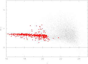
Figure 3: Colour-magnitude diagram for the galaxies detected in the R and I filters. Magnitudes are the mag_best measurement from sextractor, and colours are computed from magnitudes measured in a $3\arcsec$ aperture. Larg (red) points are the R bright galaxies (as defined in Sect. 2.4) within $300\arcsec$ of the cluster centre.

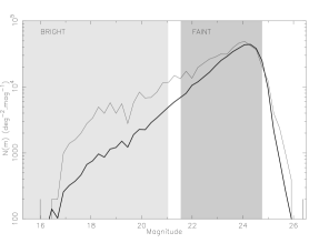
Figure 4: Number counts of galaxies in the Abell 1689 R-band image in bins of 0.23 magnitude. The thick line corresponds to counts of galaxies across the whole field, the thin line to galaxies within $300\arcsec$ from the cluster centre. The greyed area to the left (right) shows the magnitude selection for bright (faint) galaxies.

A second catalogue is created for the faint galaxies, with the following limits: $m^{*}+2.5<m<m^{\rm c}+0.5$ for the B and I-band catalogue and $m^{*}+3.5<m<m^{\rm c}+0.5$ for the R-band catalogue ($m^{\rm c}$ is the completeness magnitude which varies from filter to filter, see Table 1). These catalogues are dominated by faint and hence probably distant galaxies and are therefore considered as catalogues of background galaxies lensed by the cluster. The different cuts were adjusted in order to separate the bright (foreground) and faint (background) galaxies as much as possible without losing too many galaxies (see Fig. 4).

3 Galaxy shape measurements

The shapes of stars detected in the images provide our best estimate of the point spread function (PSF), measuring the response of the entire optical system (atmosphere + telescope optics) to a point-source. The shape of a star includes an isotropic component mainly due to atmospheric seeing, as well as an anisotropic component caused, for example, by small irregularities in the telescope guiding. The isotropic component of the PSF leads to a circularization of the images of small galaxies and thus reduces the amplitude of the measured shear. The anisotropic PSF component introduces a systematic component in galaxy ellipticities and thus causes a spurious shear measurement if not corrected (Kaiser et al. 1995). The geometric distortions of the camera and the corresponding instrumental shear are corrected during the data-reduction procedure when the image is reconstructed on a linear tangential projection of the sky on a plane.

In the case of Abell 1689, which is representative of the entire survey, the mean anisotropy of the PSF expressed in terms of ellipticity $\epsilon=(a-b)/(a+b)$ is much smaller than 0.15 in each filter (see Fig. 5).

Figure 5: Abell 1689 R-band PSF map. The length of the vectors is proportional to their ellipticity as indicated by the scale in the upper-left corner. The origin of the figure is the cluster centre. See details in §3.1.

In order to correct for both the PSF circularization and the PSF anisotropy, we use the im2shape software developed by Bridle et al. (2001). im2shape implements a Bayesian approach to measure the shape of astronomical objects by modelling them as the sum of elliptical Gaussians, convolved by the local PSF, which is also parameterized in terms of elliptical Gaussians. The minimization procedure of im2shape estimates the posterior probability distribution of the image given the model and the PSF, and Markov Chain Monte Carlo sampling gives the most probable value for each parameter, with the errors linked to the dispersion of the samples. This approach is a practical implementation of the idea presented by Kuijken (1999). im2shape is becoming increasingly popular, and has been used in a number of weak lensing applications using different instruments (Kneib et al. 2003; Cypriano et al. 2003; Faure et al. 2004).

A detailed comparison between im2shape and the KSB method is discussed by Bridle et al. (in prep.). In the following we describe in detail the procedure we implement to transform the catalogue data into source ellipticity parameters useful for a weak lensing inversion. For simplicity, only one elliptical Gaussian is used to describe both the shape of the stars and the galaxies. Indeed, as shown in Fig. 6, star profiles are well fitted by a single Gaussian. Furthermore, orientation and ellipticity (the most useful parameters for the weak lensing analysis) are relatively insensitive to the model used to describe luminosity profiles. The a posteriori justification of the validity of the choice is demonstrated by the quality of the weak lensing measurements.

3.1 Mapping the PSF distribution over the field

In a first step, im2shape is used to measure the local PSF by estimating the shapes of all the stars in the star catalogue. The resulting PSF catalogue is then inspected in detail. We first remove objects with ellipticity greater than 0.2 which mainly appear to be defects between the chips. A second cleaning pass is done to remove stars which are very different from their neighbours: if they are $>2\,\sigma$ away from the mean value of the local seeing, they are automatically rejected from the PSF catalogue. The final cleaned distortion map measured from the stars in the field is presented in Fig. 5.

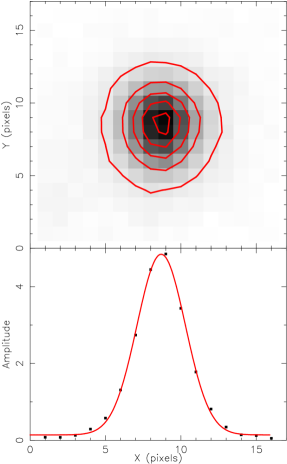
Figure 6: Top: a $16\times 16$ pixel image showing the averaged shapes of the five nearest stars to an arbitrary position (2000,2000) in the R-band image of Abell 1689. The contour levels are from 0.5 to 4.5 in steps of 1. Bottom: A cut along the $x$-axis of the image above, indicated by small squares, and a Gaussian profile fit (obtained by im2shape) shown by the solid line.

Figure 7: Left: The size distribution ($a\times b$) of the deconvolved stars. Their average size is consistent with them being point-sources.

3.2 Faint galaxy shapes

In a second step, we linearly interpolate the local PSF at each galaxy position by averaging the shapes of the five closest stars (Fig. 6). This number of stars is large enough to locally interpolate the PSF, whereas a much larger number would over-smooth the PSF characteristics. The efficiency of the PSF measurement and interpolation can be directly tested on the star catalogues. Fig. 7 shows the resulting distribution of the intrinsic sizes of stars after deconvolution with the local PSF. They are intrinsically much smaller than 0.1^th of a pixel.

im2shape then computes the intrinsic shapes of galaxies by convolving a galaxy model with the interpolated local PSF, and determine which one is the most likely by minimizing residuals. In the end, im2shape’s output gives a most likely model for the fitted galaxy characterized by its position, size, ellipticity and orientation, and errors on all of these.

Fig. 8 shows how the galaxy ellipticity distribution alters after the Im2shape correction; the effect of PSF circularization is evident.

Figure 8: The ellipticity distribution of the faint galaxies in the R-band image of Abell 1689. Left: im2shape catalogue with no PSF correction. Right: im2shape catalogue with PSF correction. The vertical line indicates the average value of the ellipticity. The effect of circularization on the faint galaxies can easily be seen.

3.3 Mean redshift of the faint galaxies

Although the photometric catalogues do not contain redshift information on the background sources, we attempt to estimate this for the population in a statistical sense. This is necessary as the relative distance of the background population and the lensing cluster is of prime importance in the quantitative scaling of the mass distribution from our weak lensing analysis. The critical parameter is the mean value of $\beta=D_{\rm LS}/D_{\rm OS}$:

$$\bar{\beta}=\frac{1}{N}\sum_{i=1}^{N}\frac{D_{{\rm LS},i}}{D_{{\rm OS},i}}$$ (1)

where $N$ is the number of faint galaxies in the catalogue and $D_{\rm LS}$ is the angular diameter distance between the lens and the source and $D_{\rm OS}$ between the observer and the source.

To compute $\bar{\beta}$ we have used a photometric redshift catalogue produced from the Hubble Deep Fields (HDF) North and South, observed with the Hubble Space Telescope (HST) (Fernández-Soto et al. 1999; Vanzella et al. 2001). This catalogue, kindly provided to us by S. Arnouts (priv. comm.), gives for each object in the HDF-N/S the apparent magnitudes and colours as well as measured spectroscopic redshift if it exists (Vanzella et al. 2002) or a photometric redshift otherwise. Similarly, each galaxy in our three CFH12k catalogues (B, R or I) has at least one entry in the corresponding photometric catalogues. Depending on the number of available entries for each galaxy (1, 2 or 3) an automatic search is done in the full HDF catalogues for the ten most similar objects in terms of magnitude and colours (correcting for the slight differences between the photometric systems of the CFH12k and WFPC2 cameras). Then the average redshift (photometric or spectroscopic if available) of these 10 objects is assigned to the galaxy. When photometric measurements are available in all three filters for an object, then this procedure crudely mimics a photometric redshift estimate, while it is a simple statistical average of photometric redshifts at a given magnitude limit otherwise. Finally, the mean redshift of each catalogue is computed, as well as the mean $\bar{\beta}$. Their values are listed in Table 1.

4 Shear measurements

We have now measured the “true” shapes of faint galaxies and estimated their mean redshift. The lensing equation for galaxy shapes can be written as:

$$\@vec{\epsilon}_{\rm I}=\frac{\@vec{\epsilon}_{\rm S}+\@vec{g}}{1+\@vec{g}^{*}\@vec{\epsilon}_{\rm S}}\quad,$$ (2)

where $\@vec{\epsilon}_{\rm I}$ and $\@vec{\epsilon}_{\rm S}$ are the complex ellipticities of the image and the source; $\@vec{g}=\@vec{\gamma}/(1-\kappa)$ is the reduced shear; $\@vec{\gamma}$ is the shear vector and $\kappa$ is the convergence (e.g.  Mellier 1999; Bartelmann & Schneider 2001). Note that both $\@vec{\gamma}$ and $\kappa$ are proportional to the distance ratio $\beta$. In the weak regime $\@vec{g}\ll 1$ the above equation simplifies to:

$$\@vec{\epsilon}_{\rm I}=\@vec{\epsilon}_{\rm S}+\@vec{g}$$ (3)

Assuming that the faint galaxy population lies at our estimated mean redshift, and assuming that galaxies have random orientations in the source plane, it is easy to see that by locally averaging a number of ellipticities we have an unbiased estimate of the reduced shear, allowing us to directly measure the mass distribution:

$$\langle\@vec{\epsilon}_{\rm I}\rangle=\langle\@vec{g}\rangle$$ (4)

The bracket $\langle\rangle$ indicate the average of a quantity near a position. However, because of the random orientation of the galaxies in the source plane, the error in the observed galaxy ellipticities and thus on the estimated reduced shear will depend on the number of galaxies averaged together to measure the shear (Schneider et al. 2000):

$$\sigma_{\@vec{g}}=\sigma_{\epsilon_{\rm I}}\approx\frac{(1-|g|^{2})\,\sigma_{\epsilon_{\rm S}}}{\sqrt{N}}$$ (5)

where $N$ is the number of galaxies used in the averaged. $\sigma_{\epsilon_{\rm S}}\sim 0.33$ (see Fig. 8) is the dispersion of the intrinsic ellipticity distribution, and the $(1-|g|^{2})$ factor is the effect of the shear on this dispersion. In the weak lensing regime, $g$ is much smaller than 1 (our measurements reach 0.1 typically, see Fig. 11), and this factor can be neglected. The error on the shear measurement is then:

$$\sigma_{\@vec{g}}\approx\frac{\sigma_{\epsilon_{\rm S}}}{\sqrt{N}}$$ (6)

Next we will explore different ways to do this averaging and constrain the cluster mass distribution.

4.1 Building the 2D shear map

The first and simplest test of the lensing influence of Abell 1689 is to compute the 2D shear maps. To compute the shear maps we average the galaxies in cells using the lensing catalogue (PSF-corrected faint galaxy catalogue). The cell size is chosen so that each cell contains about 35 galaxies. At the magnitude depth of the catalogues ($\sim 20$ galaxies arcmin^-2) this number is typically achieved for cells sizes of $80\arcsec\times 80\arcsec$. Averaging such a number of galaxies should mean that the measured average ellipticity should be small (below 0.03 from Eq. 5) and its orientation random in regions with no shear signal. Near mass peaks, we expect to see the shear vectors tangentially aligned around the centre of mass. Fig. 9 clearly shows that we detect this characteristic lensing signal around the cluster core in the R-band catalogue of Abell 1689. The signal traced by the coherent alignment of the “average” galaxy shape is represented by vectors whose length is proportional to the ellipticity and whose orientation follows the mean orientation of the galaxies in each cell. Similar shear maps are seen in the two other bands.

Figure 9: The shear map derived from the R-band image of Abell 1689. The cluster centre is marked by a “$\star$”. The circles have radii of 200″($\sim 620\,\mathrm{kpc}$), 780″($\sim 2.4\,\mathrm{Mpc}$) and 1200″($\sim 3.7\,\mathrm{Mpc}$) respectively. The inner circle corresponds to the region of strong lensing, the second one to the largest circle that lies entirely within the CFH12k field, and the outer circle marks the limit where the area outside the field becomes significant. The shear vectors are computed in cells of $80\arcsec\times 80\arcsec$, and have been smoothed by a Gaussian of 30″width (see details in §4.1).

4.2 Reconstructing the 2D mass map

We use the lensent2 code (Marshall et al. 2002) to compute the 2D non-parametric mass map of the cluster. lensent2 implements an entropy-regularized maximum-likelihood technique to derive the mass distribution within the field on a grid. The technique consists of a Bayesian deconvolution process: a trial mass distribution $\Sigma(\@vec{\theta})$ is used to generate a predicted reduced shear field through the convolution of the surface mass density by a kernel (KS93: Kaiser & Squires 1993). In contrast to KS93, lensent2 cannot produce negative feature in the mass maps leading to more physical solutions than can be obtained from direct reconstructions of the gravitational potential $\psi$. Moreover, lensent2 can include information not only from the mean shear field, but from each individual lensed galaxy with its redshift (if known). As clusters of galaxies have smooth and extended mass distributions, the values of $\Sigma$ on the field are expected to be correlated through a kernel called the Intrinsic Correlation Function (ICF). In our analysis, we provide lensent2 with a position, elliptical shape parameters (with errors) and an estimate of the redshift for each lensed galaxy (we use the mean redshift as explained in §3.3). There is then only one free parameter in the proceedure, the Intrinsic Correlation Function (ICF) which measures the correlation between mass clumps. We choose a Gaussian ICF, and let its width vary. The ICF size is optimized so that the reconstructed mass map does not contain a large number of insignificant small-scale fluctuations, although small ICFs best fit the mass peak of the cluster, while large ones best fit the wings of the extended profiles. This optimization is performed by maximizing the evidence value of each reconstruction, which is the probability to observe these data for a given ICF width. For more details on lensent2 see Marshall et al. (2002).

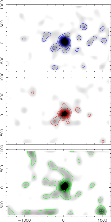
Figure 10: LensEnt2 mass reconstructions for Abell 1689 from the B (top), R (middle) and I (bottom) catalogues. The ICF is Gaussian with a width of 180″. The cluster peaks are at 1320, 1250 and $1090\ {\rm h}_{70}\ M_{\sun}.{\rm pc}^{-2}$ for B, R and I respectively. White (black) in the gray scale is set to $1\sigma$ ($5\sigma$), and contours are at 2, 3, 4 and $5\,\sigma$. $\sigma$ values are estimated as explained in §4.2. The scale is in arcsec relative to the cluster centre. A possible secondary peak is visible at [$-200\arcsec,-150\arcsec$].

The main cluster mass clump is very well detected by lensent2. The code estimates the central surface mass density of the peak, and gives its spatial configuration. Note that large ICFs smooth the main peak. Reconstructions are computed for a large set of ICFs (with scales from $60\arcsec$ to $240\arcsec$), and the best ICF width is found to be near 160–$180\arcsec$ for our dataset. An illustrative example is shown in Fig. 10 where the peak of the surface mass density is at a value of $1250\ {\rm h}_{70}\ M_{\sun}.{\rm pc}^{-2}$ in the adopted cosmology, although typical values of the critical surface mass density for massive clusters at $z_{\rm L}\sim 0.2$ are roughly around $\Sigma_{\rm c}=3200\ {\rm h}_{70}\ M_{\sun}.{\rm pc}^{-2}$ for sources at $z_{\rm S}\sim 1.0$. This is because the ICF width used here ($180\arcsec$) is much larger than the Einstein radius of the cluster ($\sim\,40\arcsec$). Therefore the smoothing process strongly attenuates the central peak density which in the case of Abell 1689 is clearly over-critical.

To assess the significance of the other mass density peaks detected in each image we randomize the orientation of the faint galaxies in the lensing catalogue, while keeping their positions and axial ratios fixed. We perform mass reconstructions of 200 randomized catalogues, and in each identify the 15 highest significance mass peaks. The statistics of these 3000 values gives a mean noise peak of $116\ {\rm h}_{70}\ M_{\sun}.{\rm pc}^{-2}$ (99, 85) above the background level (set at $100\ {\rm h}_{70}\ M_{\sun}.{\rm pc}^{-2}$ in input of lensent2) respectively in the R (B, I) images. This value is considered as the average fluctuation of the noise peaks, $\sigma$. With this definition, the cluster mass peak is detected at nearly $10\sigma$ above the background. To be formally correct, prior to randomizing their orientations we should also “unlens” the galaxies using the shear determined above and applying Eq.2. This has not been done yet for simplicity and will be explored in more detail in the next paper (Bardeau et al. in prep, paper II). However, as the lensing induced distortion is almost always very small compared to the width of the ellipticity distribution, we do not expect that this simplification will affect the estimated significance of the mass peak.

lensent2 mass reconstructions give many low significance mass peaks. For example, Fig. 10 shows that four clumps reach the 2-$\sigma$ level, but only one is above the 3-$\sigma$ level (excluding the main cluster peak). To check their reality, we can compare the reconstructions derived from the three filters (B, R and I, Fig. 10). The regions where a mass clump is detected in all three images are considered as “real” ones and can be compared to the number density map of bright cluster galaxies. Another test is to compare these clumps with any enhancement of the light distribution (§6.1), provided that the mass clumps are not associated with “dark clumps”. The multi-colour approach in our weak lensing survey provides a powerful tool to eliminate most of the inconsistencies created in the mass reconstructions from defects in the lensing catalogues. For Abell 1689, apart from the mass peak associated with the cluster, no other $>3\sigma$ peaks were detected in all three filters. A possible 2–3$\sigma$ peak is located 5′South-East of the cluster but no obvious counterpart in the galaxy distribution can be identified.

4.3 The radial shear profile

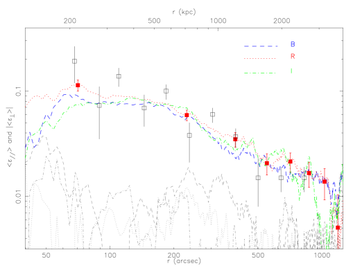
Figure 11: The tangential shear profile for Abell 1689, in the B, R and I bands. The bin width ($\Delta R$) is $160\arcsec$. A series of uncorrelated points with error bars is displayed for the R band (solid squares). Absolute values of the associated radial component $|<\varepsilon_{\perp}>|$ are indicated in grey at the bottom of the plot, showing that the signal is well detected out to $\sim 1000\arcsec$ ($\sim 3$ Mpc) from the centre. The measurements of Clowe & Schneider (2001) are also shown for comparison (open squares).

We have demonstrated that only one significant mass peak is detected in the field of Abell 1689, and that it aligns well with the cluster centre indicating it corresponds to the potential well of the cluster. In order to quantify the mass of this clump we analyse the radial distribution of the shear around this peak. Tangential and radial shear components are computed as a function of the distance to the cluster centre. They are averaged in annuli of width $\Delta R=R_{2}-R_{1}$ for a mean radius $R=\left({R_{1}}+{R_{2}}\right)/2$. $\Delta R$ is kept constant so the S/N of the shear roughly decreases as $1/\sqrt{R}$, in order to keep enough independent points at large radii (a constant S/N requires too large annuli at these radii). A quasi-continuous profile is built by using a “sliding window” with steps $\Delta r$ much smaller than $\Delta R$. In practice, we chose $\Delta R=160\arcsec$ (and $\Delta r=10\arcsec$) for the Abell 1689 R image, so about 10 independent points are included in the profile.

Fig. 11 shows the tangential and radial shear profiles from the three images of the field. The radial shear should be zero in the case of perfect data and a well chosen centre for the annuli. In practice, it can be considered as an independent estimator of measurement errors (this is also referred to as the 45 degree test). In the case of Abell 1689, the radial shear is always lower than the tangential shear out to $\sim 1100\arcsec$, arguing for good data quality in all three bands.

Note that in the very centre ($R<70\arcsec$) the shear profile appears to drop. The error bars are large due to the low number statistics: the area considered is small, reduced still further by the masking effect of the bright galaxies. Moreover the depletion of the number density of background galaxies in the center due to the magnification bias (Taylor et al. 1998) also decreases the number of observable galaxies, although this effect is only important in the inner-most annuli. These low number statistics does not completely explain the weakness of the shear: it can also be under-estimated if unlensed galaxies (such as cluster members) are included in the catalogues, which should be more likely towards the cluster core. As a consequence, the points inside $R=70\arcsec$ will not be used in the modeling of the shear profile. The measurements done by Clowe & Schneider (2001) using R band images from the ESO Wide Field Imager (WFI) are also presented in Fig. 11 for comparison. Our measurements are quantitatively in good agreement with those of Clowe & Schneider (2001). Moreover, our error bars are smaller and our points less scattered, even if we consider the different binnings. This strongly suggests that the use of im2shape in the analysis process improves significantly the shear measurements. This will be quantified in a forthcoming paper (Bridle et al. 2005, in preparation).

5 Modeling the lensing data

5.1 Description of the mass models

Three families of mass models are used to fit the measured shear profile: a singular isothermal sphere profile (SIS), a power law profile (Pow) and finally the “universal” NFW profile (Navarro et al. 1997). In addition we implemented the Aperture Mass Densitometry method (AMD) to compute a non-parametric mass profile from the shear profile itself (Fahlman et al. 1994). We recall briefly the basic equations for the mass density ($\rho$), shear ($\gamma$) and convergence ($\kappa$) profiles for the three models.

5.1.1 The Singular Isothermal Sphere model

This is the simplest mass profile used in lensing inversion. It is essentially given by the following equations:

$$\rho(r) = \frac{\sigma^{2}}{2\pi Gr^{2}}$$ (7)

$$\kappa(\theta) = \gamma(\theta)=\frac{\theta_{\rm E}}{2\theta}$$ (8)

$$\theta_{\rm E} = \frac{4\pi\sigma^{2}}{c^{2}}\frac{D_{\rm LS}}{D_{\rm S}}\quad,$$ (9)

where $\sigma$ is the velocity dispersion of the cluster. Note that once the cluster centre is fixed, this profile depends has only one free parameter ($\theta_{E}$ or equivalently $\sigma$), so only one degree of freedom is available in the fits.

5.1.2 The Power Law model

The Power Law model is a generalization of the SIS model, where the slope of the mass density profile is a free parameter (Schneider et al. 2000).

$$\gamma(\theta) = \frac{q}{2}\left(\frac{\theta}{\theta_{\rm E}}\right)^{-q}$$ (10)

$$\kappa(\theta) = \frac{2-q}{2}\left(\frac{\theta}{\theta_{\rm E}}\right)^{-q}$$ (11)

where $q$ is the slope of the Power Law ($q=1$ for the SIS model). Once the cluster centre is fixed, this model provides two degrees of freedom for fitting.

5.1.3 The NFW profile

The NFW profile is derived from fitting the density profile of numerical simulations of cold dark matter halos (Navarro et al. 1995, 1997). This theoretically-motivated profile is becoming increasingly popular in weak lensing analyses of clusters (Kneib et al. 2003) as it appears to give a reasonable description of the observed shear profiles. The mass density profile can be expressed as

$$\rho(r) = \frac{\delta_{\rm c}\rho_{\rm c}}{(r/r_{\rm s})(1+r/r_{\rm s})^{2}}$$ (12)

$$\mbox{where}\,\,\,\delta_{\rm c} = \frac{200}{3}\frac{c^{3}}{\ln(1+c)-c/(1+c)}$$ (13)

$$\mbox{and}\,\,\,\rho_{\rm c} = \frac{3H^{2}(z)}{8\pi G}\,.$$ (14)

$r_{\rm s}$ is the scale radius, $H(z)$ the Hubble parameter and $c=r_{200}/r_{\rm s}$ the concentration parameter which relates the scale radius to the virial radius $r_{200}$. This density profile is shallower than the SIS near the center but steeper in the outer parts. Similarly as the power law model, once the centre is fixed, it has two degrees of freedom: $M_{200}$ for the normalization of the mass and $r_{\rm s}$ for the scale radius, or equivalently $r_{200}$ and $c$. The details of the analytic expressions for the shear and convergence of the NFW profile can be found in King et al. (2002).

Table 2: Best fit results for the Abell 1689 R-band shear profile. For the SIS, the results are given in terms of Einstein radius ($\theta_{\rm E}$) and velocity dispersion $\sigma_{\rm los}$. For the Power Law, $\theta_{\rm E}$ is again the Einstein radius and $q$ the logarithmic slope. Finally for the universal NFW profile, $c$ is the concentration parameter and $r_{200}$ the virial radius. $M_{200}$ is the 2D-projected mass inside $r_{200}$ in units of $10^{12}\,h_{70}^{-1}\,M_{\sun}$ and $\theta_{\rm E}$ is the derived Einstein Radius. (a) refers to the fit results from Clowe & Schneider (2001), (b) from King et al. (2002). The numbers in italics assume $z_{\rm s}=1.06$.

SIS	$\sigma_{1D}\,(\mathrm{km\,s^{-1})}$	$\theta_{E}(\arcsec)$			$\chi^{2}$
	$998\pm 68$	$22.4\pm 3.0$			1.98 (1)
(a)	$1028\pm 35$	${\it 23.8\pm 1.6}$
Pow	q	$\theta_{E}(\arcsec)$			$\chi^{2}$
	$0.75\pm 0.07$	$14.6\pm 0.3$			0.637 (2)
(b)	0.88	18.0
NFW	c	$r_{200}\>({h_{70}}^{-1}$ Mpc)	$M_{200}\>(10^{12}\>{\rm M}_{\sun})$	$\theta_{E}(\arcsec)$	$\chi^{2}$
	$3.5^{+0.5}_{-0.3}$	$1.99\pm 0.25$	$1410^{+630}_{-470}$	$2.6^{+1.4}_{-0.2}$	0.334 (2)
(a)	6.0	1.83	1030	9.7
(b)	4.8	1.84	1070	5.3

5.2 Weak lensing fit

Each of the three models presented above is fitted to the data with a least square minimization over the parameter space of the models. The $\chi^{2}$ value is then:

$$\chi^{2}=\frac{1}{{\cal N}-1}\sum_{k=1}^{{\cal N}}\left(\frac{\epsilon^{\rm t}_{k}-g_{\rm model}(x_{k})}{\sigma_{k}}\right)^{2}\quad,$$ (15)

where $\cal N$ is the number of data bins, and $\sigma_{k}$ is the error on the tangential ellipticity. The error is computed in each bin as the mean error on the tangential ellipticity ($\epsilon^{\rm t}$), weighted by the number $N_{k}$ of galaxies in the bin used to do the measurement: $\sigma_{k}=\langle\sigma_{\epsilon^{\rm t}}\rangle_{k}/\sqrt{N_{k}}$.

The data in the outer regions at $r>r_{\rm max}$, where the annuli reach the borders of the field, are excluded. In practice, only the area where the tangential shear is greater than radial shear is included in the fits. Furthermore, as explained in §4.3, we also exclude the central part of the cluster. In the case of the R-band observations of Abell 1689, the fitted range corresponds to radii from $r_{\rm min}=70\arcsec$ to $r_{\rm max}=1100\arcsec$.

Table 2 summarizes the results of the fits, and Fig. 12a displays the resulting best-fit models. The lower quality of the fit by the SIS profile is easy to understand as it depends on one parameter only, contrary to the other two which are represented by two parameters. Moreover, the value of the Einstein radius deduced from the fit is significantly lower than that measured from strong lensing (which is estimated to be $\theta_{\rm E}=41\arcsec$). Note that Clowe & Schneider (2001) deduced from their weak lensing analysis a value for the Einstein radius similar to our estimate.

The fit with a power law is slightly better than the SIS as the slope of the profile appears to be shallower than isothermal, but the Einstein radius is again some 25% lower than expected (King et al. (2002) found similar results with an even lower Einstein radius).

The universal NFW profile provides the best fit to our shear profile. The concentration parameter ($c$) is slightly smaller than the values found by Clowe & Schneider (2001) and King et al. (2002), whereas the virial radius $r_{200}$ is very similar. The derived Einstein radius is however quite small and thus this model is not a good fit of the central parts of the cluster.

We conclude that total mass profile of this cluster across all angular scales is not well described by any of these simple fitting formulae and requires a more complex model, perhaps including contributions from the cluster galaxy halos and possibly a steeper central mass distribution.

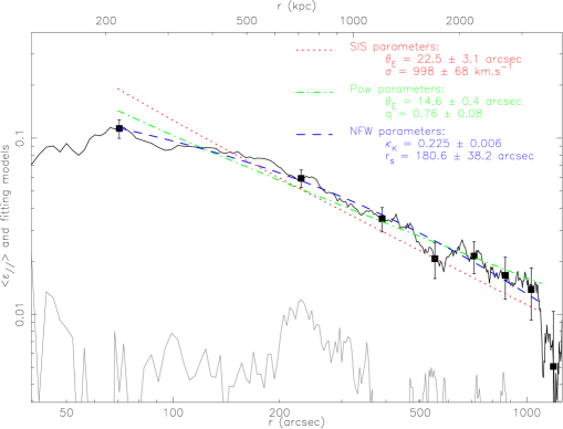
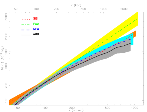
Figure 12: Top: Best fitting parameters for SIS, Power law and NFW models, for the Abell 1689 R-band shear profile. One series of uncorrelated points is shown (bin width $=160\arcsec$). Bottom: Deduced mass profiles from these models. The mass profile from the Aperture Mass Densitometry Method is also displayed, with a reference radius of 1100″. See text for details.

Fig. 12b shows the projected mass profiles from the previous fits computed with the following equation

$$M(r)=\pi r^{2}\,\Sigma_{\rm c}\,\bar{\kappa}(r)$$ (16)

where $\bar{\kappa}(r)$ is the mean dimensionless surface mass density inside radius $r$.

5.3 The Aperture Mass Densitometry method

Instead of fitting analytical formulae, we can directly integrate the measured reduced shear to determine the relative mass profile within the cluster. This direct method has been developed by Fahlman et al. (1994) and is called “Aperture Mass Densitometry” (AMD). The function $\zeta(r_{1},r_{2})$ is defined as the difference between the average convergences (or mean projected mass densities) inside the radius $r_{1}$ and within the annulus between $r_{1}$ and $r_{2}$:

$$\zeta(r_{1},r_{2}) = \bar{\kappa}(r<r_{1})-\bar{\kappa}(r_{1}<r<r_{2})$$ (17)

$$= \frac{2}{1-\left(r_{1}/r_{2}\right)^{2}}\>\int_{r_{1}}^{r_{2}}\frac{\gamma_{\rm t}}{1-\kappa(r)}\>d\ln r\quad.$$ (18)

The reconstructed mass inside the radius $r<r_{\rm max}$ is then

$$M_{\zeta}(r)=\pi r^{2}\,\Sigma_{\rm c}\;\zeta(r,r_{\rm max})\quad,$$ (19)

where $r_{\rm max}$ is the maximum radius for which we can measure the shear or the radial limit of the data. In the case of our observations of Abell 1689, we choose $r_{\rm max}\sim 1100\arcsec$, the maximum radius where annuli lie entirely within the field of view. Regarding Eq. 17, $M_{\zeta}(r)$ is only a lower limit to the true mass $M(r)=\pi r^{2}\,\Sigma_{\rm c}\,\bar{\kappa}(r)$ and should not be considered as an absolute mass determination.

The AMD mass profile is shown in Fig. 12 with the mass profiles derived by fitting the various analytical models. As expected, we find that the mass estimated from AMD is always lower than the parametric mass estimates.

6 Light distribution and mass-to-light ratio

6.1 2D light distribution

The catalogue of “bright” galaxies is expected to be dominated by cluster members, although it may also contain other bright galaxies within the field of view. Thus a density map (light density or number density) derived from this catalogue can trace the morphology of the cluster and any associated structures in its vicinity. In the case of Abell 1689, no galaxy over-densities, other than the main cluster component, are associated with any prominent peaks in the lensing mass distribution (Fig. 1).

We therefore focus on the distribution of light around the cluster centre assuming that the observed over-density is due to cluster members. First in order to build a quantitative light density map or its radial profile, it is necessary to statistically correct the catalogue for the field contamination. Fortunately, the CFH12k images are large enough so that at radii beyond 600″ from the cluster centre (2 Mpc at the cluster redshift) we can assume that the galaxy density is close to the “field” density. The mean number and light densities are therefore corrected by subtracting their minimal values estimated in the area $600\arcsec<R<1200\arcsec$.

Furthermore in order to estimate the total luminosity of the cluster and its radial profile, it is necessary to correct for the magnitude limit of the catalogue, corresponding to a cut in the cluster luminosity function (LF). The incompleteness factor $C$ is estimated as follows, the cluster LF is assumed to follow the standard Schechter luminosity function (Schechter 1976):

$$\phi(L)=\frac{{\rm d}N}{{\rm d}L}=\frac{\phi^{*}}{L^{*}}\ \left(\frac{L}{L^{*}}\right)^{-\alpha}\ {\rm e}^{-L/L^{*}}$$ (20)

Therefore the luminosity integrated in the catalogue down to a luminosity $L_{\rm inf}$ is

$$L_{\rm cat} = \int_{L_{\rm inf}}^{+\infty}L\,\phi(L)\,{\rm d}L$$ (21)

$$= \phi^{*}L^{*}\,\left[\Gamma(2-\alpha)-\Gamma(2-\alpha,L_{\rm inf}/L^{*})\right]$$ (22)

so the fraction of the luminosity not taken into account when integrating within the magnitude limits of the catalogues is written as

$$C=\frac{\Gamma(2-\alpha,L_{\rm inf}/L^{*})}{\Gamma(2-\alpha)}$$ (23)

and the total luminosity is $\displaystyle L_{\rm tot}=L_{\rm cat}/(1-C)$.

For the three bands used in this study, we need to estimate the two main parameters of the Schechter luminosity function $\alpha$ and $L^{*}$. These parameters depend on the choice of filters, on the mix of galaxy types, and on the cosmological model. The best multi-colour luminosity function determinations are presently those from the Sloan Digital Sky Survey (SDSS) early release data (Blanton et al. 2001), although they correspond to a field LF. The SDSS photometric system ($u,g,r,i,z$) is transformed to the CFH12k (Johnson) system by applying the transformations of Fukugita et al. (1996). In this paper we use the parameters of the LF summarized in de Lapparent (2003) and applied to a Sbc galaxy. Therefore the absolute magnitude $M^{*}$ in the R filter is $-21.83$ in the adopted cosmology and the slope is $\alpha_{\rm R}=1.20$. This includes also the k-correction at redshift $0.18$, computed with the galaxy evolutionary code by Bruzual & Charlot (2003).

Finally, the correction factors $1/(1-C)$ are applied to $L_{\rm cat}$ to obtain the total integrated magnitude for the B, R and I catalogues, with the magnitude ranges defined in Sect. 2.4. The precise values derived are summarized in Table 3.

Table 3: The photometric parameters of the luminosity function in B, R and I filters for our adopted cosmology: $H_{0}=70\,\mathrm{km\,s^{-1}\,Mpc^{-1}}$, $\Omega_{\rm m}=0.3$ and $\Omega_{\Lambda}=0.7$. The distance modulus is $m-M=39.70$ or equivalently the luminosity distance is $D_{\rm L}=872\,\mathrm{Mpc}$, at $z_{\rm A1689}=0.18$. $1/(1-C)$ is the correction factor applied to the integrated luminosity of the catalogues to determine the total luminosity of the cluster.

	B	R	I
k-correction	1.06	0.16	0.16
$M^{*}-5\log h_{70}$	-20.47	-21.83	-21.54
$\alpha$	1.30	1.20	1.25
$m^{*}\ (z=0.18)$	20.29	18.03	17.32
$1/(1-C)$	1.28	1.11	1.27

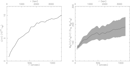
Figure 13: Left: luminosity profile for the bright galaxy catalogue, for R-band image of Abell 1689, corrected for background contamination. See Sect. 6.1 for details. Right: $M_{R}/L_{R}$ ratio as a function of radial distance from the cluster centre. The mass profile is estimated from the best fit NFW parameters. The filled region indicates the errors on the profile.

6.2 Comparison of mass and light: M/L radial profile

Using the best-fitting NFW model for the observed shear profile, the $M/L$ profile is computed by dividing the luminosity profile, estimated from the bright galaxies catalogue, by the mass profile. The field contamination in this catalogue is estimated by measuring the minimum of the surface brightness density between $600\arcsec$ and $1200\arcsec$ from the cluster center. Fig. 13a displays this integrated luminosity profile for the R-band image. Note that the $L_{\rm R}$ values adopt the correction factor discussed in the previous section.

Fig. 13b displays the $M_{\rm R}(<r)/L_{\rm R}(<r)$ profile with error bars estimated from the errors on the mass profile only. The $M/L$ increases from a low value (near $100\pm 10\,h_{70}\,(M/L)_{\sun}$ at $400\,\mathrm{kpc}$ from the centre) and flattens out beyond $\sim 1\,{\rm Mpc}$ at a value near $160\pm 40\,h_{70}\,(M/L)_{\sun}$. This behaviour is independent of the filter considered. It does however depend slightly on the background correction at large radius, and on the detailed mass modeling in the inner part of the cluster. In particular, as we derived a relatively small Einstein radius compared to that determined from strong lensing, we are likely to be underestimating the mass in the central regions, which would suggest an even flatter $M/L$ profile towards the centre.

Beyond $\sim 1\,\mathrm{Mpc}$ the $M/L$ ratio found in Abell 1689 is consistent with being constant with radius. This result is similar to the findings of Kneib et al. (2003) in their lensing analysis of the cluster Cl 0024+1654 ($z=0.39$), both in the radial distribution and in the normalization. For comparison, $(M/L)_{\rm R}$ at large radii in the Coma cluster is found to be $170\pm 50\,(M/L)_{\sun}$ from dynamical analysis (Geller et al. 1999; Rines et al. 2001). Similar profiles for mass and light on 1–5 Mpc scales are expected if cluster assembly is largely governed by infalling groups and if no strong mass segregation occurs in the cluster.

In their sample of 12 distant clusters ($0.17<z<0.56$) Smail et al. (1997) found a mean value of $(M/L)_{V}^{\rm all}=126_{-77}^{+147}\,(M/L)_{\sun}$ ($h=0.7$) in the cluster cores, where the superscript all refers to the entire population of the clusters, not only early-type galaxies. Given the colour index ($V-R$) of a mean Sa galaxy at redshift 0.18, this corresponds to $(M/L)_{R}^{\rm all}=102_{-62}^{+119}\,(M/L)_{\sun}$. Since our bright galaxies catalogue is dominated by elliptical galaxies (Fig.3), we expect to find a lower luminosity thus their $M/L$ value is consistent with our findings.

7 Discussion and Conclusion

In this paper, we describe the methodology used to analyze a multi-colour wide-field imaging survey of 11 X-ray luminous clusters. The goal of our survey is to constrain the mass distribution in clusters of galaxies using weak gravitational lensing. The main elements of the data analysis are: the use SExtractor for object detection and photometry to provide well-defined object catalogues. A “stars” catalogue is used to determine the PSF locally, a “bright galaxies” catalogue is defined to trace the distribution of cluster members and a “faint galaxies” catalogue is constructed which should comprise background galaxies. The magnitude limits of each catalogue are determined with respect to the observational constraints such as the limiting magnitudes of the available images as well as physical constraints related to the magnitude distribution in the clusters at a given redshift. In order to determine the “true” PSF-deconvolved shape properties of the background (lensed) galaxies we use the im2shape package developed recently for the purpose of improving the quality of shear measurements, including a correct treatment of the measurement errors (Bridle et al. 2001). We then reconstruct the mass distribution by computing the shear profile and either fitting it with parametric mass models like the NFW mass profile or deducing the relative profile directly with the non-parametric Aperture Mass Densitometry method. Both methods are found to be consistent. We also show a 2D mass reconstruction using the lensent2 software (Marshall et al. 2002) and applying it to the three images taken through the three filters. Finally we compute the $M/L$ ratio as a function of radius, again in the three photometric bands. The three filters are used independently for most of the processing steps in order to confirm the significance of the results (comparison of shear profiles and mass maps). They give quantitatively consistent results, further demonstrating the robustness of our method. The images in the three filters are used jointly to estimate the background galaxies’ redshift distribution and so provide a correct normalization of the mass determination.

We apply this method to the well-known cluster Abell 1689 as a test-case. We find only one significant mass peak in the mass reconstructions, corresponding to the cluster itself. This is consistent with preliminary results from a large spectroscopic survey of Abell 1689 and its outskirts (Czoske 2004), which shows that the environment of this cluster is remarkably smooth and quiet. We also compare our results to previous work by Clowe & Schneider (2001) who used an independent data set and the methods from Kaiser et al. (1995) and Kaiser & Squires (1993) for their galaxy shape measurements and mass reconstruction. Within the errors both reconstructions agree very well. The same is true for the $M/L$ determination, which is consistent with previous findings. Moreover we are able to build a $M/L$ profile which in the case of Abell 1689 shows a near constant behaviour at large radius with a possible decrease close to the center. This suggests that mass traces light at least in the outskirts of the cluster. The drop of $M/L$ in the cluster centre may be due to an underestimate of the mass in the centre, due to increasing contamination of the background galaxy catalogue by cluster members diluting the lensing signal. The flat $M/L$ profile in the infall region of the cluster indicates that the association between mass and light has already been achieved outside the cluster and the effect of the cluster environment on the mass-to-light ratio of infalling galaxies and groups is minor. This supports the picture of a hierarchical assembly of clusters.

For the results presented here we did not make use of the colour information available from multi-band imaging to separate cluster from background galaxies which makes our results directly comparable to those of Clowe & Schneider (2001). However Clowe (2003) presented an updated mass reconstruction for Abell 1689, this time using colours derived from our CFH12k images. The colour information resulted in an improved removal of cluster galaxies from his background galaxy catalogue, increasing both $r_{200}$ and $c$ for his best-fit NFW model and better agreement of the weak lensing mass profile with that derived from strong lensing. We will include colour selection of the different galaxy catalogues in a forthcoming paper aimed at comparing in great detail all the mass estimates at different scales in Abell 1689: velocity distribution of the galaxies, X-ray mass maps, strong lensing in the center of the cluster and weak lensing at larger scales. Provided the dynamics of the cluster is well understood this should give a consistent picture of its mass distribution and components. This is the main goal of the pan-chromatic survey which is conducted by our group on intermediate redshift X-ray clusters.

Finally, we will present a global study of our results based on the application of the present methodology to the whole cluster catalogue, with a discussion of the statistical properties of such clusters. A better understanding of the global properties of the mass distribution in rich clusters of galaxies will provide profound insights into the growth of structure in the Universe.