Theoretical modelling of the diffuse emission of $\gamma$-rays from extreme regions of star formation: The case of Arp 220

Abstract

Astrophys.J.617:966-986, 2004

Our current understanding of ultraluminous infrared galaxies suggest that they are recent galaxy mergers in which much of the gas in the former spiral disks, particularly that located at distances less than 5 kpc from each of the pre-merger nuclei, has fallen into a common center, triggering a huge starburst phenomenon. This large nuclear concentration of molecular gas has been detected by many groups, and estimates of molecular mass and density have been made. Not surprisingly, these estimates were found to be orders of magnitude larger than the corresponding values found in our Galaxy. In this paper, a self-consistent model of the high energy emission of the super-starburst galaxy Arp 220 is presented. The model also provides an estimate of the radio emission from each of the components of the central region of the galaxy (western and eastern extreme starbursts, and molecular disk). The predicted radio spectrum is found as a result of the synchrotron and free-free emission, and absorption, of the primary and secondary steady population of electrons and positrons. The latter is output of charged pion decay and knock-on leptonic production, subject to a full set of losses in the interstellar medium. The resulting radio spectrum is in agreement with sub-arcsec radio observations, what allows to estimate the magnetic field. In addition, the FIR emission is modeled with dust emissivity, and the computed FIR photon density is used as a target for inverse Compton process as well as to give account of losses in the $\gamma$-ray scape. Bremsstrahlung emission and neutral pion decay are also computed, and the $\gamma$-ray spectrum is finally predicted. Future possible observations with GLAST, and the ground based Cherenkov telescopes are discussed.

1 Introduction

In a recent letter (Torres et al. 2004), it was shown that some luminous and ultra-luminous infrared galaxies (LIRGs and ULIRGs) are plausible sources for GLAST and the next generation of Cherenkov telescopes (HESS, MAGIC, VERITAS). In order to show that, the $\gamma$-ray flux output of neutral pion decay, under a set of reasonable and commonly used –albeit numerous– simplifications, was computed. An obvious caveat of this earlier approach is that it was not possible to predict an spectrum of the ULIRGs-emitted high-energy radiation, but rather only integrated fluxes. Also, correlation at lower frequencies was not pursued. Here, a detailed, self-consistent model of the radio, IR, and $\gamma$-ray emission from Arp 220, the nearest ULIRG, minimizing as much as possible –based on current multiwavelength observations– any freedom in parameter selection, is presented.

To that end, a set of numerical codes that allow the computation of multiwavelength spectra from regions of star formation, molecular clouds, and other environments, was developed. Being this the first application of such program –whose validation was run against previously published results– some of the details of what it implements are discussed in a technical Appendix. The code set, dubbed ${\cal Q}$-diffuse, solves the diffusion-loss equation for electrons and protons, and finds the steady state distribution for these particles subject to a complete set of losses in the interstellar medium (ISM). It computes secondaries from hadronic interactions (neutral and charged pions) and Coulomb processes (electrons), and gives account of the radiation or decay products that these particles produce. Secondary particles (photons, muons, neutrinos, electrons, and positrons) that are in turn produced by pion decay are calculated too, using a new set of paramaterizations of the differential cross sections, developed recently by Blattnig et al. (2000). These parameterizations are discussed here in some detail as well. Additional pieces of the code compute the dust emissivity, and the IR-FIR photon density, which is used both as target for inverse Compton scattering and to model the radiation at lower frequencies. Finally, opacities to $\gamma\gamma$ and $\gamma Z$ processes are computed, as well as absorbed $\gamma$-ray fluxes, using the radiation transport equation.

Previous studies of diffuse high energy emission, and of electron and positron production, with different levels of detail and aims, go back to the early years of $\gamma$-ray astronomy. A summary of these first efforts can be found in the review paper by Fazio (1967) and in the book by Ginzburg and Syrovatskii (1968). See also the pioneering works by Ramaty & Lingenfelter (1968), Maraschi et al. (1968), and Stecker (1977), among many others. Secondary particle computations have a similarly long, and obviously related history see, e.g., Stecker (1969; 1973), Orth and Buffington (1976), and others quoted below. More recent efforts, related mainly to the modelling of supernova remnants and the Galactic center, include those of Schlickeiser (1982), see also his book and references quoted therein (Schlickeiser 2002), Aharonian et al. (1994), Drury et al. (1994), Atoyan et al. (1995), Aharonian & Atoyan (1996), Moskalenko & Strong (1998), Strong & Moskalenko (1998), Markoff et al. (1999), and Fatuzzo & Melia (2003); although making here a comprehensive list is not intended. Here, the general ideas used by Paglione et al. (1996) and Blom et al. (1999), when modelling nearby starbursts galaxies, are followed. These, in turn, closely track Brown & Marscher’s (1977) and Marscher & Brown’s (1978), regarding their studies of close molecular clouds. The current implementation seems to introduce some further improvements. Apart from using different parameterizations for pion cross sections, which were argued to better agree with experiments, as mentioned above, the code set uses the full inverse Compton Klein-Nishina cross section, computes secondaries without resorting to parameterizations which are valid only for Earth-like cosmic ray (CR) intensities, fixes the photon target for Compton scattering starting from modelling of the observations in the FIR, and considers opacities to $\gamma$-ray scape.

The rest of this paper is organized as follows. In the next Section, LIRGs and ULIRGs as $\gamma$-ray sources are discussed. Section 3 is an account of Arp 220 phenomenology. The description of the dust emission model and the supernova explosion rates that were implemented are discussed there as well. Section 4 is a discussion of the solution to the diffusion-loss equation in a general case. Section 5 shows how emissivities of secondary particles were computed. Section 6 discusses the steady distribution of particles in the different components of Arp 220, together with the resulting radio and $\gamma$-ray spectrum. Some concluding remarks are given at the end.

2 LIRGs & ULIRGs as $\gamma$-ray sources

ULIRGs are recent galaxy mergers in which much of the gas in the former spiral disks, particularly that located at distances less than $\sim 5$ kpc from each of the pre-merger nuclei, has fallen into a common center, triggering a huge starburst phenomenon (see Sanders & Mirabel 1996 for a review). The size of the inner regions of ULIRGs, where most of the gas is found, can be as small as a few hundreds parsecs; there, an extreme molecular environment is found.

This large nuclear concentration of molecular gas has been detected in the millimeter lines of CO by many groups. Using Milky Way molecular clouds to calibrate the conversion factor between CO luminosity and gas mass soon led to the paradox that most, if not all, of the dynamical mass was gas (e.g., for Arp 220, see Scoville et al. 1991). In some extreme cases, the derived gas mass exceeded the dynamical mass estimation, which unambiguously showed caveats in any of the assumptions. However, Downes et al. (1993) showed that in the central regions of ULIRGs, much of the CO luminosity comes from an intercloud medium that fills the whole volume, rather than from clouds bound by self gravity. Hence, the CO luminosity of ULIRGs traces the geometric mean of the gas and the dynamical mass, rather than just the gas. The Milky Way conversion factor, being relevant for an ensemble of giant molecular clouds (GMCs) in an ordinary spiral galaxy, seems to overestimate the gas mass of ULIRGs. Solomon et al. (1997), Downes & Solomon (1998), Bryant & Scoville (1999), and Yao et al. (2003) have argued for that in the case of ULIRGs, conversion factors between gas mass and CO luminosities can be $\sim$5 times smaller than for the Milky Way. Even with such corrections, the amount of molecular gas in ULIRGs is huge, typically reaching 10¹⁰ M_⊙.

The existence of large masses of dense interstellar gas suggests that all LIRGs may have $\gamma$-ray luminosities orders of magnitude greater than normal galaxies. This assumption was explored by Torres et al. (2004), who found that the expectation of LIRGs to shine at $\gamma$-rays is not automatically granted. It is not only the amount of gas (actually, the amount of gas divided by the distance to its location) what yields to detectability at high energies, but rather it is the amount of gas that is found at high density, and thus that it is prone to form stars and be subject to significant enhancements of cosmic rays. Using the HCN survey recently released by Gao & Solomon (2004a,b), Torres et al. noted that there are a group of 7 LIRGs (out of 31 in that sample) that, being gas-rich (i.e., CO-luminous) but having normal star formation efficiency $L_{\rm IR}/L_{\rm CO}$ (e.g., $L_{\rm HCN}/L_{\rm CO}<0.06$), are not expected to be detected in $\gamma$-rays (at least under the simple modelling explored by these authors). Some examples are NGC 1144, Mrk 1027, NGC 6701, and Arp 55. These galaxies are using the huge molecular mass they have in creating stars at a normal star formation rate (SFR). Cosmic ray enhancements are, most likely, not high enough to lead to detection, given the distance to these objects.

Then, even when they may appear far from Earth to be detected at high energies, perhaps it is the extreme environment of star-bursting ULIRGs the most appealing to study. One such galaxy stands alone among all others: Arp 220 (RA_J2000, DEC_J2000=15 34 57.24, +23 30 11.2). Although LIRGs are the dominant population of extragalactic objects in the local ($z<0.3$) universe at bolometric luminosities above $L>10^{11}$ L_⊙, they are still relatively rare (Sanders & Mirabel 1996). The luminosity function of LIRGs suggest that there should be only one object with $L_{\rm FIR}>10^{12}$ L_⊙ out to a redshift of 0.033. Indeed, Arp 220 ($z=0.018$) is the only ULIRG in the 100 Mpc sphere. As such, Arp 220 is probably the best studied ULIRG.

3 Arp 220

Arp 220’s center has two radio-continuum and two IR sources, separated by $\sim 1$ arcsec (e.g., Scoville et al. 1997, Downes et al. 1998, Soifer et al. 1999, Wiedner et al. 2002). The two radio sources are extended and nonthermal (e.g., Sopp & Alexander 1991; Condon et al. 1991; Baan & Haschick 1995), and likely produced by supernovae in the most active star-forming regions. CO line, cm, mm-, and sub-mm continuum (e.g., Downes & Solomon 1998) as well as recent HCN line observations (e.g., Gao & Solomon 2004a,b) are all consistent with these two sources being sites of extreme star formation and having very high molecular densities. Arp 220 is also an OH megamaser galaxy, as first discover by Baan et al. (1982). The 1.6 GHz continuum emission of Arp 220 has a double component structure too, with the two components being separated by about 1 arcsec and located at the same positions as the 1.4 GHz, the 4.8 GHz, and the 1.3 mm emission (see, e.g., Rovilos et al. 2002, 2003). In the eastern nucleus, the position of the maser coincide with that of the continuum. In the western one, the OH maser emission arises from regions north and south from the continuum (Rovilos et al. 2002, 2003).

Different characteristics of the two extreme starbursts and the molecular disk, some of which are used as input in our modelling, are given in Tables 1 and 2, as derived by Downes and Solomon (1998). Other authors, particularly those reporting results with sub-arcsec angular resolution (e.g., Soifer et al. 1999, Wiedner et al. 2002), while confirming the general features of the modelling of the central region proposed by Downes and Solomon, may present differences in the details. For instance, the densities quoted by Weidner et al. (2002) are slightly larger than those used here. Sakamoto et al. (1999) have proposed, also based on CO observations with sub-arcsec resolution, that the western and eastern nuclei are not spherically symmetric but are counter-rotating, $\sim 100$ pc disks, with $\sim 10^{9}$ M_⊙ masses (see their figure 5). This model seems to have some support in VLBI observations of OH masers (Rovilos et al. 2003). Regarding the $\gamma$-ray emission from Arp 220, such changes in geometry will not yield any significant change in the results, although would probably also imply higher densities that those consider here. To fix the scenario on the conservative side, Downes and Solomon’s (1998) results are adopted, and for consistency, their assumed value of Arp 220 luminosity distance (72.3 Mpc) is also used. Modifications to the cosmological model would produce an order 1% percent change in the results.

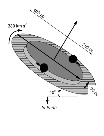
Figure 1: Geometry and different components in the model of Arp 220. Two central spherical nuclei are extreme regions of star formation, and co-rotate with the molecular disk.

The assumed geometry of the central region of Arp 220 is sketched in Figure 1, not to scale. The CO disk is inclined 40^∘ from face-on, Arp 220-west (one of the extreme starbursts) is assumed spherical, with a radius of 68 pc. Similarly, Arp 220-east has a radius of 110 pc. The disk thickness is 90 pc. The rotational curve of the CO disk indicates a dynamical mass of at least $12\times 10^{9}$ M_⊙ interior to the outer disk radius, of 480 pc, which corresponds to the central bulge mass of a large spiral like the Milky Way. The gas mass in each of the two extreme starburst nuclei is at least $6\times 10^{8}$ M_⊙. Their individual FIR luminosities are $\sim 3\times 10^{11}$ L_⊙. About half of the Arp 220 FIR luminosity comes from the molecular disk. The masses of the two extreme starbursts are negligible in comparison with the mass that controls the motion of the molecular disk. Furthermore, the two nuclei of Arp 220 have radial velocities indicating that they take part in the general disk rotation, i.e., that they share the general rotation in the potential of the old bulge, and are dominated by the disk gravity, not their self. There is no observational evidence –radio, infrared, or optical– that they contain old stars, so that the estimated mass in new stars could just be the total mass minus the gas mass (Downes & Solomon 1998). The gas density quoted in Table 1 and 2 corresponds only to estimates of molecular hydrogen, thus the total density ought to be larger. The contribution of atomic hydrogen is to be considered subdominant, as it is in the inner disk of the Milky Way (see e.g. Mirabel & Sanders 1988; 1989). The total nuclei density is derived from the H₂ number density estimation, taking into account heavier and lighter species. Also, it is important to note that the models in the paper by Downes & Solomon (1998) are for distributed gas, but there is denser gas in the star forming cores, giving rise to HCN and CS lines. Most of the CO comes from the distributed medium, so that total masses have to be corrected upwards (e.g. Gao & Solomon 2004a,b). Equally, the density might be higher that the estimate used here, perhaps especially in the disk. Thus, from the point of view of target mass, our estimates of, for instance, neutral pion decay $\gamma$-rays or charged pion decay electrons, could be regarded as a conservative estimation.

Table 1: Some properties of Arp 220’s extreme starbursts.

Property	West	East
Geometry	sphere	sphere
Radius [pc]	68	110
Average gas density (H2) [cm-3]	$1.8\times 10^{4}$	$8.0\times 10^{3}$
Luminosity (FIR) [L⊙]	$0.3\times 10^{12}$	$0.2\times 10^{12}$

Table 2: Some properties of Arp 220’s disk.

Property	Value
Geometry	cylinder
Thickness [pc]	90
Outer radius [pc]	480
Inclination from face-on	40o
Average gas density within the outer radius (H2) [cm-3]	$1.2\times 10^{3}$
Luminosity (FIR) [L⊙]	$0.7\times 10^{12}$

Table 3: Main symbols used in the paper, meaning, and units.

Symbol	Meaning	Unit
$b(E)$	rates of energy loss	GeV s-1
$\tau(E)$	confinement timescales	s
$Q(E)$	emissivities	particles GeV-1 s-1 cm-3
$N(E)$	distributions	particles GeV-1 cm-3
$J(E)$	intensities	particles GeV-1 cm-2 s-1 sr-1
$F(E)$	differential fluxes	particles GeV-1 cm-2 s-1
$F(E>\bar{E})$	integral fluxes above $\bar{E}$	particles cm-2 s-1

Additional evidence supporting the dominance of star forming processes in Arp 220, as compared with what would be the influence of an active but hidden black hole, come from the hard X-ray band/soft $\gamma$-ray bands. Dermer et al. (1997) have reported OSSE observations of Arp 220, finding a $2\sigma$ upper limit in the 50-200 keV range (see below). Previous hard X-ray limits on Arp 220, by HEAO-1 and Ginga (Rieke 1988) also ruled out a bright hard X-ray source ($>{\rm few}\,\times 10^{-11}$ erg cm^-2 s^-1). Iwasawa et al. (2001) reported observations with Beppo-Sax, which detected X-ray emission up to 10 keV but imposed only an upper limit at higher frequencies. It is also worth noticing that there is no strong Fe K line detection from Arp 220, although a tentative detection of an emission line at 6.5 keV, at the 2$\sigma$-level, has been made (Clements et al. 2002).

Starburst phenomena were used by Shioya, Trentham & Tanigushi (2001) and Iwasawa et al. (2001) to explain the X-ray properties of Arp 220, although the existence of a heavily obscured AGN is not yet ruled out. Chandra results (Clements et al. 2002) show that the nuclear X-ray emission in Arp 220 is confined to a sub-kiloparsec scale region, in contrast to other starburst galaxies. Its spectrum indicates that X-rays are more likely produced by one or more low luminosity, heavily obscured, low mass AGN, or by several high luminosity X-ray binaries, or ultra luminous X-ray sources, rather than by supernovae. Therefore the co-existence of a subdominant AGN with a dominant starburst is still plausible. Of course, even when a weak AGN would contribute now only with $\sim 1\%$ to the bolometric luminosity, in the dense nuclear region of Arp 220, the black hole is bound to grow and increase in luminosity as the system evolves. Proof of the existence of a black hole in Arp 220 (or otherwise) is then important in our understanding of the possible relationship between quasars and ULIRGs.

3.1 The supernova rate in Arp 220

18 cm VLBI (3 $\times$ 8 milliarcsec resolution) continuum imaging of Arp 220 has revealed the existence of more than a dozen sources with 0.2$-$1.2 mJy fluxes (Smith et al. 1998), mostly in the western nucleus. These compact radio sources were interpreted as supernova remnants. This interpretation is consistent with a simple starburst model for the IR luminosity of Arp 220 (Smith et al. 1998b), having a constant SFR in the range 50$-$100 M_⊙ yr^-1, and a supernova explosion rate in the range ${\cal R}\sim 1.75-3.5$ yr^-1. Smith et al. (1998) suggest the adoption of a supernova explosion rate of 2 yr^-1, with an uncertainty that could make it be twice this value. A radio supernova would thus appear in Arp 220 at least once every six months, and several individual SNRs would be visible at any given moment.

A model of the hidden nucleus was constructed using starburst99 (Shioya, Trentham & Tanigushi 2001) for which the star formation rate derived was 267 M_⊙ yr^-1; 160 M_⊙ yr^-1 [107 M_⊙ yr^-1] of which correspond only to the western [eastern] extreme starburst. For equal assumptions on the IMF slope, the lower and upper limits on star masses, and the mass needed for a star to evolve to a supernova, as compared with Smith et al.’s (1998) work, a supernova rate of $\sim 4$ yr^-1 is derived using this model, which is consistent with, but at the upper end of, previous estimates.

Van Buren and Greenhouse (1994) developed, starting from Chevalier’s (1982) model for radio emission from supenova blast waves expanding into the ejecta of their precursor stars, a direct relationship between the FIR luminosity and the rate of supernova explosions. The result is ${\cal R}=2.3\times 10^{-12}L_{\rm FIR}/L_{\odot}$ yr^-1. They proved that the supernova rate resulting from this relation was consistent with that derived from the star formation rates in M82, NGC 253, and other galaxies. In the case of ULIRGs, Manucci et al. (2003) derived a similar expression. The latter authors found, by studying a sample of 46 LIRGs and detecting 4 supernovae, that the supernova rate can be approximately given by ${\cal R}=(2.4\pm 0.1)\times 10^{-12}L_{\rm FIR}/L_{\odot}$ yr^-1, in nice agreement with Van Buren and Grennhouse’s results. Mattila and Meikle (2001) have also obtained a similar value for the proportionality factor.

In the case of Arp 220, the total so-computed supernova rate is ${\cal R}=2.8\pm 0.1$ yr^-1, which is compatible with previous results. The mentioned relationship between $L_{\rm FIR}$ and ${\cal R}$ gives then the possibility of distributing the Arp 220 total supernova rate into the different components (i.e., disk, western and eastern nuclei) according to their weight in the FIR emission, and this is the approach followed here. As shown below, this rate, together with the measured geometry of the system, fixes the primary injection proton distribution. As compared with Local Group Galaxies, the supernova rate in Arp 220 is $\sim 300$ times larger (e.g., see the compilation produced by Pavlidou and Fields 2001, where the maximum rate occurs for M31, and it is 0.9 explosions per century).

3.2 Dust emission

The continuum emission from Arp 220, at wavelengths between $\sim 1$ cm and $\sim 10$ microns, was measured by Woody et al. (1989), Eales et al. (1989), Scoville et al. (1991), Carico et al. (1992), and Rigopoulou (1996), among others. These observations did not distinguish, due to angular resolution, the different geometrical components described in Figure 1, and were fitted with different models for dust emission. In particular, Scoville et al. (1991) already found that the continuum emission was mainly produced thermally, by dust, and thus that it could be modelled with a spectrum having an emissivity law $\nu^{\sigma}B(\epsilon,T)$. Later, already with arcsec imaging, Scoville et al. (1997), Downes and Solomon (1998), and Soifer et al. (1999) distinguished the contribution of the two extreme starburst regions, and obtained results compatible with previous measurements. However, the dust emission modelling is strongly dependent on sizes, temperatures, and emissivity indices of each of the emission regions, so that for a small variation in any of these parameters, large changes in the predicted fluxes of the components may result. This produces a modelling degeneracy, acknowledged already by Soifer et al. (1999). They provide a multicomponent fit for the dust emission of Arp 220, and several possible scenarios, all compatible with observations, were presented. These scenarios were recently re-analyzed by Gonzalez-Alfonso et al. (2004), on the light of ISO-LWS observations.

Entering into too many details to represent the dust emission would increase the number of parameters without a way of distinguishing between different models with data now at hand. In addition, since forthcoming $\gamma$-ray missions telescopes will not resolve the different components, it is not really possible to relate subarcsec FIR modelling with arcmin $\gamma$-ray observations. In the spirit of Scoville et al. (1991), the simplest possible scenario is herein adopted; i.e., the FIR emission is produced by dust in each of the components, and that it is radiated with a single temperature and emissivity law. The model (sum of the three contributions) derived to fit the data ($\sigma=1.5$, $T=42.2$ K, see Appendix for details) provides an excellent description of the observations, as can be seen in Figure 2. Note that, if anything, this model may underestimates slightly what would be the real photon density, particularly in the molecular disk, what implies that this computation will not overestimate the inverse Compton contribution. In any case, at high energies, in the dense environment of Arp 220, inverse Compton emission is sub-dominant as compared with pion decay $\gamma$-rays (see below).

Note that there are two points that deviates from the theoretical curve in Figure 2. The first is at the lowest frequencies, where the dust emission model predicts less emission than observed. Indeed, this behavior is correct, since at that frequency there is a non-negligible non-thermal contribution coming from synchrotron radiation as well as a thermal contribution coming from thermal bremsstrahlung, computed below. This makes for this difference in the fit. At the highest frequencies, the dust emission predicts less emission than observed too, which is also correct, since at high frequencies the source is optically thinner and better described by a blackbody.

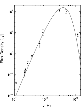
Figure 2: Data points and dust emission model assumed in this paper for the IR-FIR radiation from Arp 220. Data points come from literature quoted in the text, with typical errors of $\sim$20%. The theoretical curve is based on the assumption that the whole IR-FIR luminosity is produced by dust located at each of the components, emitting with a single temperature (42.2 K) and emissivity index (1.5).

4 Diffusion-loss equation

The general diffusion-loss equation is given by (see, e.g., Longair 1994, p. 279; Ginzburg & Syrovatskii 1964, p. 296)

$$-D\bigtriangledown^{2}N(E)+\frac{N(E)}{\tau(E)}-\frac{d}{dE}\left[b(E)N(E)\right]-Q(E)=-\frac{\partial N(E)}{\partial t}.$$ (1)

In this equation, $D$ is the scalar diffusion coefficient, $Q(E)$ represents the source term appropriate to the production of particles with energy $E$, $\tau(E)$ stands for the confinement timescale, $N(E)$ is the distribution of particles with energies in the range $E$ and $E+dE$ per unit volume (see Table 3 for units), and $b(E)=-\left({dE}/{dt}\right)$ is the rate of loss of energy. The functions $b(E)$, $\tau(E)$, and $Q(E)$ will then be different depending on the nature of the particles (i.e., electrons – positrons, and protons, are subject to different kind of losses and are also produced differently), but the form of the equation will be the same for both. Here, two terms are to be neglected: in the steady state, ${\partial N(E)}/{\partial t}=0,$ and the spatial dependence is considered to be irrelevant, so that $D\bigtriangledown^{2}N(E)=0.$ This is reasonably under the assumption of a homogeneous distribution of sources.

Eq. (1) can be –formally– solved, as can be proven by direct differentiation, by using the Green function

$$G(E,{E^{\prime}})=\frac{1}{b(E)}\exp\left(-\int_{E}^{E^{\prime}}dy\frac{1}{\tau(y)b(y)}\right),$$ (2)

such that for any given source function, or emissivity, $Q(E)$, the solution is

$$N(E)=\int_{E}^{E_{\rm max}}d{E^{\prime}}Q({E^{\prime}})G(E,{E^{\prime}}).$$ (3)

Note that the integral in $E^{\prime}$ is made on the primary energies which, after losses, produce secondaries with energy $E$. In general, however, $G(E,{E^{\prime}})$ has not a close analytical expression, and neither does $N(E)$. Numerical integration techniques are then needed to compute Eq. (3).

Instead of directly assuming a steady state particle distribution, it is considered that the latter is the result of an injection distribution being subject to losses and, eventually, to secondary production, in the ISM. In general, the injection distribution may be defined to a lesser degree of uncertainty when compared with the steady state one, since the former can be directly linked to observations, e.g., to the supernova explosion rate. Such evolution of the injection spectrum will be given as a solution of Eq. (1), with appropriate $b(E)$ and $\tau(E)$ functions.

The total rate of energy loss herein considered for protons is given by the sum of that involving ionization and pion decay, as it is discussed in the Appendix. An example of these rates of energy loss is shown in Figure 3 (left panel). For electrons, the total rate of energy loss considered is given by the sum of those involving ionization, inverse Compton scattering, bremsstrahlung, and synchrotron radiation, as it is also discussed in the Appendix. These rates of energy loss are shown in the right panel of Figure 3 for a particular choice of system parameters. In that figure, the inverse Compton losses are computed in the Thomson approximation. The full Klein-Nishina cross section is used while computing photon emission, and either Thomson or extreme Klein-Nishina approximations, as needed, are used while computing losses. This approach proves to be accurate, while significantly reduces the computational time.

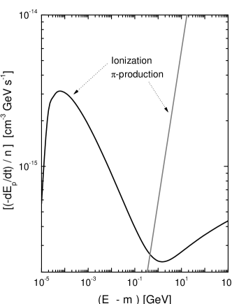
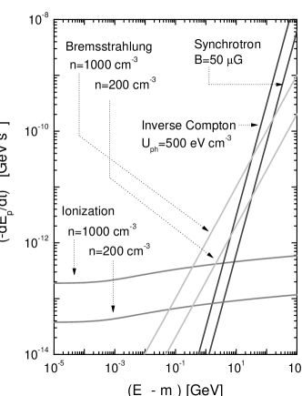
Figure 3: Example of the rate of energy loss for protons (left panel) and electrons (right panel) considered in this work. Protons losses are mainly produced by ionization and pion production. Both are proportional to the medium density, and this is factored out (in units of cm^-3). Electrons losses correspond to synchrotron and bremsstrahlung radiation, inverse Compton scattering, and ionization. A set of random parameters is assumed for this example –shown in the figure–, additionally to the assumption that the average density of the photon target is $\bar{\epsilon}=1$ eV.

The confinement timescale will be given by the characteristic escape time in the homogeneous diffusion model (Berezinskii et al. 1992, p. 50-52 and 78) $\tau_{D}={R^{2}}/({2D(E)})={\tau_{0}}/(\beta(E/{\rm GeV})^{\mu}),$ where $\beta$ is the velocity of the particle in units of $c$, $R$ is the spatial extent of the region from where particles diffuse away, and $D(E)$ is the energy-dependent diffusion coefficient, whose dependence is assumed $\propto E^{\mu}$, with $\mu\sim 0.5$. $\tau_{0}$ is the characteristic escape time at $\sim$ 1 GeV. Note that, whereas the form of $\tau_{D}$ is assumed the same for both protons and electrons, its value at a fixed energy is only the same for particles with equal Lorentz factors (and thus equal $\beta$). The total escape timescale will also take into account that particles can be carried away by the collective effect of stellar winds and supernovae. In general, it is reasonable to suppose that this timescale ($\tau_{c}$) is within one order of magnitude of $\tau_{0}$. $\tau_{c}$ is indeed $\sim R/V$, where $V$ is the collective wind velocity. Thus, in general, $\tau^{-1}(E_{p})=\tau_{o}^{-1}\beta\left({E}/{{\rm GeV}}\right)^{\mu}+{\tau_{c}}^{-1}.$

Note that if $Q(E)$ is a power law, $N(E)$ scales linearly with its normalization. However, there is no immediate scaling property with the density of the ISM, which enters differently into the several expressions of losses that conform $b(E)$.

5 Computation of secondaries

For the production of secondary electrons, only knock-on and pion processes are taken into account. These processes dominate by more than an order of magnitude the production of electrons at low and high energies, respectively, when compared with neutron beta decay (see, e.g., Marscher & Brown 1978 and Morfill 1982 for discussions on this issue).

5.1 Electrons from knock-on (or Coulomb) interactions

Knock-on (or Coulomb) collisions are interactions in which the proton CR transfers an energy far in excess of the typical binding energy of atomic electrons, so producing low-energy relativistic electrons. The cross section for knock-on production was calculated by Bhaba (1938) and subsequently analyzed by Brunstein (1965) and Abraham et al. (1966), among others. The differential probability for the production of an electron of energy $E_{e}$ and corresponding Lorentz factor $\Gamma_{e}=E_{e}/m_{e}c^{2}$, within an interval $(\Gamma_{e}-d\Gamma_{e},\Gamma_{e}+d\Gamma_{e})$, produced by the collision between a CR of particle species $j$, and energy factor $\Gamma_{j}$ and a target of charge $Z_{i}$ and atomic number $A_{i}$ is, in units of grammage,

$$\Phi(\Gamma_{e},\Gamma_{j})d\Gamma_{e}=\left[\frac{2\pi N_{0}Z_{i}r_{e}^{2}Z_{j}^{2}}{A_{i}(1-\Gamma_{j}^{-2})}\left(\frac{1}{(\Gamma_{e}-1)^{2}}-\frac{s\left(\Gamma_{j}+\frac{s^{2}+1}{2s}\right)}{(\Gamma_{e}-1)\Gamma_{j}^{2}}+\frac{s^{2}}{2\Gamma_{j}^{2}}\right)\right]\,d\Gamma_{e}\;{\rm cm}^{2}\;{\rm g}^{-1}.$$ (4)

Here $N_{0}$ is the Avogadro’s number, $r_{e}=e^{2}/mc^{2}=2.82\times 10^{-13}$ cm is the classical radius of the electron, and $s=m_{e}/(A_{i}m_{p})\sim 1/1836$ (see below). Note that the probability for interaction is proportional to $Z_{i}/A_{i}$. Then, it will suffice to assume that the interstellar medium is 90% hydrogen and 10% Helium and neglect the contribution of higher atomic numbers. This approximation introduces negligible error. Contributions by various nuclei in the colliding CR population are more important, since the probability for interaction is proportional to $Z_{j}^{2}$. If the total contribution of all primaries with charge $Z\geq 2$ relative to that of protons is $\sim 0.75$, then $\sum_{i}\sum_{j}\Phi(\Gamma_{e},\Gamma_{j})\sim 1.75\,\Phi(\Gamma_{e},\Gamma_{p}).$

The maximum transferable energy in this kind of collisions is (e.g., Abraham et al. 1966) $\Gamma_{\rm max}=1+\left(\Gamma_{p}^{2}-1\right)/\{s\left(\Gamma_{p}+[{s^{2}+1}/{2s}]\right)\}.$ Thus, the maximum possible energy is limited only by the maximum value of $\Gamma_{p}$, while the minimum proton Lorentz factor that is needed to generate an electron of energy $E_{e}$ is fixed by solving the inequality $\Gamma_{e}\leq\Gamma_{\rm max}$. The result is that $\Gamma_{p}\geq\Gamma_{1}$, with $\Gamma_{1}=[1/2]s(\Gamma_{e}-1)+\sqrt{1+\frac{1}{2}(1+s^{2})(\Gamma_{e}-1)+\frac{1}{4}s^{2}(\Gamma_{e}-1)^{2}}.$ With this in mind, the source function for knock-on electrons to be considered in the diffusion-loss equation is then given by

$$Q_{\rm knock}(E_{e})\sim 1.75\;m_{p}\;n\;4\pi\;\int_{E_{1,p}}\Phi(E_{e},E_{p})\,J_{p}(E_{p})\,dE_{p}\;,$$ (5)

where $E_{1,p}=\Gamma_{1}\,m_{p}$, $\Phi(E_{e},E_{p})=\Phi(\Gamma_{e},\Gamma_{p})/m_{e}$, i.e. energies, instead of Lorentz factors, are used to write the final integral, and $J_{p}$ is the CR proton intensity ($J_{p}(E)=(c\beta/4\pi)N(E)$).

If the CR intensity is described by a power law whose exponent is exactly an integer or half of an integer, i.e., $-2,-2.5,-3,$ etc., lengthy analytical expressions for the knock-on source function can be obtained. This is no longer true for generic power laws. Examples of the results for the computation of the knock-on source function are given in Figure 4.

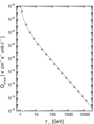
Figure 4: Left: Knock-on source function for different CR intensity $J_{p}(E_{p})=A(E_{\rm kin}/{\rm GeV})^{\alpha}$ protons cm^-2 s^-1 sr^-1 GeV^-1. We have normalized the source function by taking an ISM density ($n=1$ cm^-3) and unit normalization of the incident proton spectrum, $A$=1. Curves shown are, from top to bottom, the corresponding to $\alpha=-2.1,-2.5$, and $-2.7$. Right: Simple power law fit of the knock-on source function for $\alpha=-2.5$. Similar fits can be plotted for all values of $\alpha$, see text for details.

As it is shown there, and was first proposed by Abraham et al. (1966), the behavior of the knock-on source function can be well represented by a power law of the form $Q_{\rm knock}(E_{e})\sim constant\times(\Gamma_{e}-1)^{-b}{\rm electrons}\;{\rm cm}^{-3}\;{\rm s}^{-1}\;{\rm GeV}^{-1}.$ An example of such a description can be found in the right panel of Figure 4, where the spectrum obtained using Eq. (5) is superposed to the fit.

5.2 $\gamma$-rays from neutral pion decays

The $\pi^{0}$ emissivity resulting from an isotropic intensity of protons, $J_{p}(E_{p})$, interacting with –fixed target– nuclei with number density $n$, through the reaction $p+p\rightarrow p+\pi^{0}\rightarrow p+2\gamma$, is given by (e.g., Stecker 1971)

$$Q_{\pi^{0}}(E_{\pi^{0}})=4\pi n\int_{E_{th}(E_{\pi^{0}})}dE_{p}\,J_{p}(E_{p}){d\sigma(E_{\pi^{0}},E_{p})\over dE_{\pi^{0}}}\;,$$ (6)

where $E_{p}(E_{\pi^{0}})$ is the minimum proton energy required to produce a pion with total energy $E_{\pi^{0}}$, and is determined through kinematical considerations. ${d\sigma(E_{\pi^{0}},E_{p})/dE_{\pi^{0}}}$ is the differential cross section for the production of a pion with energy $E_{\pi^{0}}$, in the lab frame, due to a collision of a proton of energy $E_{p}$ with a hydrogen atom at rest. The $\gamma$-ray emissivity is obtained from the neutral pion emissivity $Q_{\pi^{0}}$ as

$${Q_{\gamma}(E_{\gamma})}_{\pi}=2\int_{E_{\pi^{0}}^{min}(E_{\gamma})}dE_{\pi^{0}}{Q_{\pi^{0}}(E_{\pi^{0}})\over(E_{\pi^{0}}^{2}-m_{\pi^{0}}^{2}c^{4})^{1/2}}$$ (7)

where $E_{\pi^{0}}^{min}(E_{\gamma})=E_{\gamma}+m_{\pi^{0}}^{2}c^{4}/(4E_{\gamma})$ is the minimum pion energy required to produce a photon of energy $E_{\gamma}$ (e.g., Stecker 1971).

Recently, Blattnig et al. (2000) developed parameterizations of the differential cross sections regulating the production of neutral and charged pions. On one hand, Blattnig et al. have presented a parameterization of the Stephens and Badhwar’s (1981) model by numerically integrating the Lorentz-invariant differential cross section (LIDCS). The expression of such parameterization is divided into two regions, depending on the (laboratory frame) proton energy (Blattnig et al. 2000).

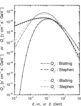
Figure 5: Left: $\pi^{0}$ and $\gamma$-emissivities computed using Blattnig et al.’s (2000) and Stephen and Badhwar’s (1981) parameterizations. Right: Discrepancies between cross section models are shown as the ratio of the emissivities of secondary neutral particles. In both panels, $n=1$ cm^-3, and an Earth-like proton spectrum ($\propto E^{-2.75}$) are assumed.

On the other hand, Blattnig et al.’s new parameterization has, particularly in the case of neutral pions, a much simpler analytical form. It is given by

$$\frac{d\sigma(E_{\pi^{0}},E_{p})}{dE_{\rm\pi^{0}}}=10^{-27}e^{\left(-5.8-{1.82}/{(E_{p}-m_{p})^{0.4}}+{13.5}/{(E_{\rm\pi^{0}}-m_{\rm\pi^{0}})^{0.2}}-{4.5}/{(E_{\rm\pi^{0}}-m_{\rm\pi^{0}})^{0.4}}\right)}{\rm cm}^{2}\;{\rm GeV}^{-1}$$ (8)

which ease the computation of the pion spectrum as compared to the isobaric (Stecker 1971) or scaling models (Stephens & Badwhars 1981), see, e.g. Dermer (1986), although yet requiring numerical integration subroutines. [Recall that rest masses and energies must be given, in the last equation, in units of GeV.] Blattnig et al.’s parameterization were not yet applied to compute $\gamma$-ray emission. Then, a brief analysis can prove useful. Specifically, the computed pion decay emissivity using the new Blattnig et al.’s (2000) parameterization (Eq. 8) is herein compared with that corresponding to the Stephen and Badhwar’s (1981) one, assuming the same proton injection and density as in Dermer (1986).

Using Eq. (7), it is possible to see that under the Blattnig et al. new parameterization, the number of pions produced at low ($E_{\pi^{0}}-m_{\rm\pi^{0}}<10^{-2}$ GeV) energies is significantly less than that produced using the alternative model. Fig. 6 of Blattnig et al. (2000) shows that their new differential cross section parameterization decreases rapidly at low energies and goes to approximately zero at 10 MeV. Fig. 5 of the same paper shows that Stephen and Badhwar’s cross section, instead, is much larger at very low pion energies (see Blattnig et al. 2000b for further details). Noteworthy, this fact, however, does not substantially affect the $\gamma$-ray emission in the region of interest since to produce a photon of energy $\sim$10^-2 GeV, pions of minimum energy of $\sim 0.5$ GeV are required, and at these energies, the pion spectrum using both approaches agrees reasonable well (i.e. the $\gamma$-ray spectrum is within an order of magnitude at all energies). This comparison is shown in detail in the two panels of Figure 5.

Regrettably, it seems not possible to answer which parameterization is the correct one at low energies with current experimental data (see Blattnig et al. 2000 for a discussion). The problem being that the shapes of the two spectral distributions, (${d\sigma(E_{\pi^{0}},E_{p})}/{dE_{\rm\pi^{0}}}$), look quite different even when both original LIDCSs have a similar fit to the data at low transverse momentum of the produced pion, where the cross section is the greatest, and that both integrate to the same total cross section. Notwithstanding, at high transverse momentum, Stephen and Badwhars’s parameterization overpredicts the cross section for several orders of magnitude, and Blattnig et al.’s form is preferred, (Eq. 8). Then, for neutral pion decay computations, Eq. 8 is adopted in our computations. In the case of charged pions, Badwhar’s (1977) LIDCS is considered the most reliable at all energies, and then their corresponding spectral distributions are adopted, see below.

5.3 Electrons and positrons from charged pion decay

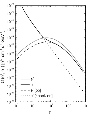
Figure 6: Left: $\pi^{\pm}$-emissivities produced using Blattnig et al.’s (2000) parameterizations of Bhadwar et al.’s (1977) spectral distribution, ${d\sigma}/{dE}$. Right: $e^{\pm}$-emissivities. In the case of electrons, the total emissivity adds up that produced by knock-on interactions, which dominates at low energies. In both panels, $n=1$ cm^-3, and an Earth-like proton spectrum ($\propto E^{-2.75}$) are assumed.

Positron production occurs through muon decay in the reactions $p+p\rightarrow X+\pi^{+}$ with the pion then decaying as $\pi^{+}\rightarrow\mu^{+}+\nu_{e}+\bar{\nu}_{\mu}$. Electron production occurs, similarly, through, $p+p\rightarrow X+\pi^{-}$ with the pion then decaying as $\pi^{-}\rightarrow\mu^{-}+\bar{\nu}_{e}+\nu_{\mu}$. Considering first the latter decays in the frame at rest with the pion, conservation of energy and momentum imply ${p_{\mu}}^{\prime}=\left({{E_{\mu}}^{2}}^{\prime}-{m_{\mu}}^{2}\right)^{1/2}=[{m_{\pi}}^{2}-{m_{\mu}}^{2}]/{2m_{\pi}},$ where $m_{\mu,\pi}$ are the masses of the muon and pion, respectively, $E$ are total energies and the prime is used to represent the pion rest frame. This implies that the energy of the pion in such frame is ${\Gamma_{\mu}}^{\prime}={{E_{\mu}}^{\prime}}/{m_{\mu}}=[{m_{\pi}}^{2}+{m_{\mu}}^{2}]/[2m_{\pi}m_{\mu}]\sim 1.04.$ The value of ${\Gamma_{\mu}}^{\prime}$ implies, as long as the velocity of the pion in the laboratory frame is not exceedingly small ($\Gamma_{\pi}>1.04$), that the muon is practically at rest in the rest frame of the pion, and that as seen from the lab, $\Gamma_{\mu}\sim\Gamma_{\pi}$. Then, per unit Lorentz factor, the muon emissivity is equal to that of the pion $Q_{\pi^{+}}(\Gamma_{\pi^{+}})=Q_{\mu^{+}}(\Gamma_{\mu^{+}})$, $Q_{\pi^{-}}(\Gamma_{\pi^{-}})=Q_{\mu^{-}}(\Gamma_{\mu^{-}}).$ The charged pion emissivity resulting from an isotropic distribution of protons $J_{p}(E_{p})$ interacting with –fixed target– nuclei found with number density $n$ can be computed as that of the neutral pions, by just changing the spectral distribution

$$Q_{\pi^{\pm}}(\Gamma_{\pi^{\pm}})=4\pi n\int_{\Gamma_{th}(\Gamma_{\pi^{\pm}})}d\Gamma_{p}\,J_{p}(\Gamma_{p}){d\sigma(\Gamma_{\pi^{\pm}},\Gamma_{p})\over d\Gamma_{\pi^{\pm}}}\;,$$ (9)

where $\Gamma_{p}(\Gamma_{\pi^{\pm}})$ is the minimum proton Lorentz factor required to produce a pion (either positively or negatively charged) with Lorentz factor $\Gamma_{\pi^{\pm}}$. Thus, knowledge of the spectral distribution ${d\sigma(\Gamma_{\pi^{\pm}},\Gamma_{p})/d\Gamma_{\pi^{\pm}}}$ secures knowledge of the muon emissivity. Use of the new parameterizations of the Bhadwar et al. (1977) LIDCS (Blattnig et al. 2000). Figure 6, left panel, shows an example of the $\pi^{+}$– and $\pi^{-}$–emissivity. The electron and positron emissivities are computed as a three-body decay process (see, e.g. Schlickeiser 2002, p. 115):

$$Q_{e^{\pm}}(\Gamma_{e^{\pm}})={\int_{1}}^{{\Gamma_{e}}^{\prime{\rm max}}}d{\Gamma_{e}}^{\prime}\frac{1}{2}\frac{P({\Gamma_{e}}^{\prime})}{\sqrt{{\Gamma_{e}}^{\prime 2}-1}}\int_{\Gamma_{\mu 1}}^{\Gamma_{\mu 2}}d{\Gamma_{\mu}}\frac{Q_{\mu^{\pm}}(\Gamma_{\mu^{\pm}})}{\sqrt{{\Gamma_{\mu}}^{2}-1}}.$$ (10)

Here ${{\Gamma_{e}}^{\prime{\rm max}}}=104$, $\Gamma_{\mu 1,\mu 2}=\Gamma_{e^{\pm}}{\Gamma_{e}}^{\prime}\mp\sqrt{{\Gamma_{e}}^{\prime 2}-1}\sqrt{{\Gamma_{e}}^{2}-1},$ and the function $P$ is $P({\Gamma_{e}}^{\prime})=2{{\Gamma_{e}}^{\prime}}^{2}\left[3-\frac{2{{\Gamma_{e}}^{\prime}}}{{{\Gamma_{e}}^{\prime{\rm max}}}}\right]/{({{\Gamma_{e}}^{\prime{\rm max}}})^{3}}.$ Figure 6, right panel, shows an example of the $e^{+}$– and $e^{-}$–emissivity, as implemented in the code. These results are compatible with previous computations.

6 Steady distributions, emissivities, and magnetic fields in Arp 220

6.1 Protons

The injection proton emissivity is here, following Bell (1978), assumed to be a power law in proton kinetic energies, with index $p$ (herein $p=2.2$),

$$Q_{\rm inj}(E_{\rm p,\,kin})=K\left(\frac{E_{\rm p,\,kin}}{\rm GeV}\right)^{-p},$$ (11)

where $K$ is a normalization constant. This normalization is to be obtained from the total power transferred by supernovae into CRs kinetic energy within a given volume

$$\int_{E_{\rm p,\,kin,\,min}}^{E_{\rm p,\,kin,\,max}}Q_{\rm inj}(E_{\rm p,\,kin})E_{\rm p,\,kin}dE_{\rm p,\,kin}=-K\frac{E_{\rm p,\,kin,\,min}^{-p+2}}{-p+2}\equiv\frac{\sum_{i}\eta_{i}{\cal P}{\cal R}_{i}}{V}$$ (12)

where it was assumed that $p\neq 2$, used the fact that $E_{\rm p,\,kin\,min}\ll E_{\rm p,\,kin,max}$ in the second equality, and defined ${\cal R}_{i}$ ($\sum_{i}{\cal R}_{i}={\cal R}$) as the rate of supernova explosions in the star forming region being considered, $V$ being its volume, that transfer a fraction $\eta_{i}$ of the supernova explosion power (${\cal P}\sim 10^{51}$ erg) into CRs. The summation over $i$ takes into account that not all supernovae will transfer the same amount of power into CRs (alternatively, that not all supernovae will release the same power). The rate of power transfer is assumed to be in the range 0.05 $\lesssim\eta_{i}\lesssim$ 0.25 (e.g., Torres et al. 2003 and references therein), uniformly distributed. Then, taking a ten-piece histogram, $\sum_{i}\eta_{i}{\cal R}_{i}=0.165{\cal R}$. Note that $E_{\rm p,\,kin,min}$ is also fixed by requiring that the minimum kinetic proton energy with which a CR escapes from a shock front be larger than $2m_{p}v_{s}^{2}$ (Bell 1978). For shock velocities of the order of 10^3-4 km s^-1, this is in the range of a few MeV. A value of 10 MeV is taken to fix numerical constants, although its precise value is not a relevant parameter in this problem.

These assumptions imply that the injection is fixed as

$$Q_{\rm inj}(E_{p})=\!\left[\frac{{\cal P}\times{\sum_{i}\eta_{i}{\cal R}_{i}}\times V^{-1}}{\rm GeV\,{\rm s}^{-1}\,{\rm cm}^{-3}}\right]\!\![p-2]\!\!\left[\frac{E_{\rm p,\,kin,\,min}}{\rm GeV}\right]^{p-2}\!\!\left[\frac{E_{p}-m_{p}}{\rm GeV}\right]^{-p}\!\!{\rm GeV}^{-1}\,{\rm cm}^{-3}\,{\rm s}^{-1}.$$ (13)

The numerical solution of the diffusion-loss equation for protons, subject to the losses described in the Appendix, is shown in Figure 7. It is assumed that the unknown diffusion timescale is proportional to $\tau_{o}=1$ Myr for the extreme starburst regions, and to $\tau_{o}=10$ Myr for the much larger volume occupied by the disk. The chosen $\tau_{o}$ is a factor of 2–10 less than that estimated for our Galaxy or M33 (e.g., Gaisser 1990, Duric et al. 1995), and parallels that obtained in the study of NGC 253 and M82, which are a galaxies presenting a more similar environment to Arp 220 (Paglione et al. 1996, Blom et al. 1999). The shorter residence timescale for the extreme starburst regions actually makes for a conservative assumption: if erring, it would be (slightly) underestimating the $\gamma$-ray flux. The previous values will stand for the assumed model of Arp 220, but others are explored in the middle panel of Figure 7. There, corresponding to the western nucleus, the ratio between the proton distribution obtained with $\tau_{o}=10,0.5,$ and 0.1 Myr, and that obtained with the adopted model in this paper ($\tau_{o}$=1 Myr), is shown. Unless in the extreme case of very low $\tau_{o}$, the steady distribution is not significantly sensitive to this parameter. Differences increase with energy, and amount to less than 5% at 1 TeV, what is practically unobservable regarding the $\gamma$-ray output. The latter can increase or decrease slightly, depending on the value of $\tau_{o}$ adopted, and uncertainties in other parameters can wash out this effect completely. For the case with $\tau_{o}=0.1$ Myr, there would be a reduction of the relativistic distribution of protons by a factor of 2 at the highest energies. However, such a low value of $\tau_{o}$ is not favored: it represents a residence time two orders of magnitude shorter than that of our Galaxy, and it would largely dominate over the radiative timescales, what is not the case in dense molecular clouds (see, e.g., the appendix of the work by Marscher & Brown 1978).

Ionization (pion) losses dominates at low (high) energy, and this change in the dominant mechanism for the energy loss produces the kink that appears in the curves of Figure 7 around a kinetic energy of 300 MeV. Note that the steady distribution in each of the components is similar (and actually, slightly larger for the extreme starburst regions) despite of their different sizes. This implies that the number of protons per unit energy is more than 50 times larger in the extreme starburst regions than in the molecular disk.

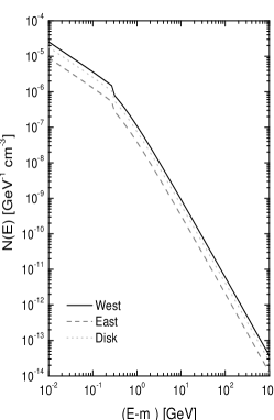
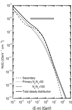
Figure 7: Left: Steady distribution of protons in each of the components of Arp 220. Middle: Testing the influence of the parameter $\tau_{0}$ in the determination of the proton steady distribution. Right: Example for a steady distribution of electrons and positrons in a western-like starburst (with $B=10$ mG). The contribution to the total steady distribution of the primary and secondary electrons and positrons is separately shown. The horizontal rectangle shows the region of electron kinetic energies where the steady distribution of secondary electrons is larger than that of the primary electrons. It is in this region of energies where most of the synchrotron radio emission is generated.

6.2 Electrons and positrons

With the steady proton spectrum shown in Figure 7, left panel, the knock-on, and pion-generated electron and positron emissivities are computed. To these emissivities, an injection electron spectrum is also added, which is assumed as the proton injection times a scaling factor; the inverse of the ratio between the number of protons and electrons, $N_{p}/N_{e}$ (e.g., Bell 1978). This ratio is about 100 for the Galaxy, but could be smaller in star forming regions, where there are multiple acceleration sites. For instance, Völk et al. (1989) obtain $N_{p}/N_{e}\sim 30$ for M82. $N_{p}/N_{e}=100$ is assumed for the disk and $N_{p}/N_{e}=50$ is assumed for both of the starburst nuclei. These values stand for a conservative approach, e.g. the more the primary electrons, the larger the inverse Compton $\gamma$-ray emission.

With such emissivities, and using the diffusion-loss equation with corresponding losses, the leptonic steady distribution is calculated. The inverse Compton scattering losses make use of the photon density in the FIR derived above, and additionally, a value of magnetic field is assumed to compute the influence of synchrotron losses. The difference between the primary and secondary electrons steady distributions, for a western-like extreme starburst with a magnetic field of 10 mG is shown in the right panel of Figure 7.

6.3 Radio emission and magnetic fields

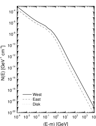
Figure 8: Left: Influence of the magnetic field in the determination of the steady state electron distribution in a western-like starburst region. Right: Final steady leptonic distributions whose radio emission fit observations. It is with these distributions that leptonic $\gamma$-ray emissivities are computed.

The influence of the magnetic field upon the steady state electron distribution is shown in Figure 8. The greater the field, the larger the synchrotron losses –what is particularly visible at high energies, where synchrotron losses play a relevant role. Thus, the larger the field the smaller the steady distribution. These effects evidently compete between each other in determining the final radio flux. In order to model the different components of Arp 220, the magnetic field is required to be such that the radio emission generated by the steady electron distribution in each region (see Appendix) is in agreement with the observational radio data. This is achieved by iterating the feedback between the choice of magnetic field, the determination of the steady distribution, and the computation of radio flux [and at the same time taking into account free-free emission and absorption processes, see Appendix]. These distributions are shown in the right panel of Figure 8. To reproduce the observational radio data, it is important to note that whereas free-free emission is subdominant when compared with the synchrotron flux density, free-free absorption plays a key role at low frequencies, where it determines the opacity.

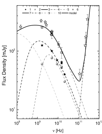
Figure 9: Radio and FIR emission of the different components of Arp 220. 1, 2, 3 (also compiled by Downes & Solomon 1998, see their figure 19), and 4 (see Figure 2) are observational data points corresponding to the western and eastern nuclei, the disk, and the total FIR flux density, respectively. The curves close to each of these set of points is the result of the modelling. The curve with no observational data points nearby is the model prediction for the molecular disk; its emission is summed into the thickest black curve, which is the result of adding all components and the final prediction of the model for the radio emission.

The radio emission produced by these distributions is shown in Figure 9, together with observational data. The beam size for the different data points varies (see, e.g., table 3 of Soop & Alexander 1991) and unless in the cases of sub-arcsec observations, in general, the beam contains a region larger than the one modelled herein. However, it is expected that most of the radio emission comes from the central and more active regions of the galaxy, and thus a reasonable model of the nuclear environment should reproduce most of the radiation. The magnetic field and the free-free critical frequencies for each of the components are given in Table 4. The solid curve in Figure 9 is, then, not a fit to the data, but the prediction of the theoretical model with the chosen magnetic field. This prediction takes into account the presence of secondary electrons, which, as can be seen in the right panel of Figure 7, dominate the steady distribution in the energy range where most of the radio emission is produced. The FIR observations and modelling shown in Figure 9 is that already presented in Figure 2: it can be noted here that the observational data point at $\nu\sim 10^{11}$ Hz is accounted for when considering the contribution of the non-thermal radio emission at that frequency.

The lowest frequency data point in each of the components is used to define the critical frequency for the free-free opacity. This is a function of the emission measure and temperature. But since there is only one observational point at such low values of $\nu$, the reliability of the determination of the critical frequency is lower than that of the magnetic field. The latter is the main responsible for the fixing of the steady electron distribution and the prediction of the radio emission at higher frequencies, where several observations are available for comparison.

To exemplify the uncertainty in the critical frequency determination, consider the western nucleus. In that case, the lowest frequency point could be thought of as being part of the free-free opacity-produced decay of the radio emission curve, or as part the non-thermal synchrotron trend, if the critical frequency is lower. An intermediate situation is adopted here. This also influences the value of critical frequency adopted for the disk –forcing the critical frequency in that case to be lower than that in the extreme starbursts in order to be in agreement with the first data point of the total radio curve. For the eastern nucleus, it is apparently clear that the first data point –obtained at high angular resolution– is already opacity-dominated, since its value is less than the contiguous data at higher frequency. In any case, both nuclei seem to have a relatively high critical frequency, particularly when compared with the disk, what would be in agreement with them being stronger star forming regions. The critical frequencies mentioned in Table 4 can be obtained with temperatures between 5 and 10 $\times 10^{3}$ K, and EM values between 10⁴ and 10⁷ pc cm^-6, the smaller EM corresponding to the disk. Similar values of critical frequencies, temperatures, and emission measures were used to model the radio emission in the case of the starburst galaxy NGC 253 (Paglione et al. 1996).

Table 4: Parameters for radio modelling.

Component	Magnetic Field	Critical Frequency
western starburst	6.5 mG	0.38 GHz
eastern starburst	4.5 mG	2.86 GHz
disk	280 $\mu$G	0.07 GHz

Consider now the analysis of the magnetic field results, which appear, as said, to be more stable against model degeneracy. It is worth noticing that not much is known about the magnetic field in ULIRGs, except for upper limits ($\sim 5$ mG), obtained with Zeeman splitting measurements of four southern OH megamaser galaxies (Killeen et al. 1996). This study, being for a more active star-forming galaxy, is compatible with these estimates and favor the ideas regarding the existence of such high fields in extreme starbursts (e.g., Smith et al. 1998).

It is to be remarked that for both the western and eastern nuclei, the minimal energy argument does not seem to hold. With the magnetic field strength given in Table 4, and the relativistic steady state populations of Figures 7 (left panel) and 8 (right panel), only the molecular disk is in magnetic energy equipartition. This appears to be a similar scenario -although more extreme- to that found for the interacting galaxy NGC 2276, where the magnetic field seems not in energy equipartition with cosmic rays either (Hummel & Beck 1995).

The magnetic field in the extreme starbursts is compatible with those measured nearby supernova remnants in the Galaxy (Koralesky et al. 1998; Brogan et al. 2000), where field strengths between 0.1 and 4 mG were found. These fields strengths were interpreted as being an ambient magnetic field compressed by the supernova remnant. The same mechanism could be thought of for Arp 220’s western and eastern nucleus. The disk magnetic field, in turn, is compatible with the result for molecular clouds presented by Crutcher (1991), what is in agreement with the disk itself being thought of as a gigantic molecular cloud with the gas filling all the medium.

Similarly high values of magnetic fields ($B>800\,\mu$G) were necessary to produce the observed collimated outflows in ULIRGs, and particularly in Arp 220, as a resultant of a strong starburst environment (Gouveia Dal Pino & Medina Tanco 1999). Finally, the overall magnetic field distribution bears some resemblance with our own Galactic Center. There, in a few dense gas clouds about 2 pc north of the Galactic center, field strengths in the milligauss range were derived from Zeeman measurements (see Beck 2001 for a review; Plante et al. 1994; Yusef-Zadeh et al. 1996). The average field in Sgr A complex is, in analogy with the disk value, restricted to less than 0.4 mG (Reich 1994). The non-detection of the Zeeman effect in the OH lines (Uchida and Güsten 1995) also indicates a relatively weak general magnetic field into which clouds with strong fields are embedded.

6.4 $\gamma$-ray emissivity and first estimation of fluxes

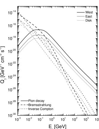
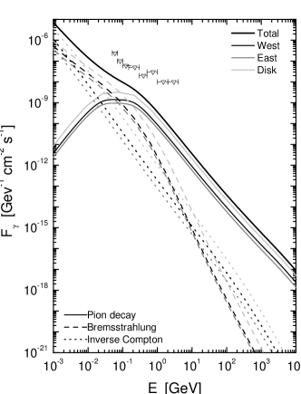
Figure 10: Left: Bremsstrahlung, inverse Compton, and pion decay emissivity of $\gamma$-rays in the different components of Arp 220. Right: Differential fluxes without considering opacity effects. The down-triangles are EGRET upper limits.

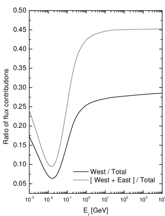
Figure 11: Relative importance of the extreme starburst regions as compared with the total $\gamma$-ray flux predicted from Arp 220. No opacities are herein considered although its inclusion would not change this result.

In the left panel of Figure 10 the bremsstrahlung, inverse Compton, and pion decay $\gamma$-ray emissivities of the different components of Arp 220, is shown. These results are derived for the model which is in agreement with radio and IR-FIR observations. At energies above 100 MeV, pion decay $\gamma$-rays is the dominant contribution, as expected. Clearly, the emissivity of high energy photons is the largest in the western extreme starburst, the most active region of star formation. It is followed by the eastern nuclei, and in a subdominant role, by the molecular disk. The differential flux, shown in the right panel of Figure 10 without considering absorption effects, shows the effect of volume. The disk $\gamma$-ray flux is the largest, and the nuclei are now subdominant. Nevertheless, only the western starburst provides more than one fourth of the total $\gamma$-ray flux (similar to the weight of its contribution in the IR band; although note, however that the total luminosity in the $\gamma$-ray band is much less than in the IR). The relative importance of the western and eastern nuclei in the total $\gamma$-ray radiation budget is shown in Figure 11. Upper limits to the differential photon flux from Arp 220 are also shown in Figure 10. These limits were obtained from an analysis of 4 years of EGRET data (see Cillis et al. 2004) and are in agreement with model predictions.

6.5 $\gamma$-ray escape

The opacity to $\gamma\gamma$ pair production with the photon field which, at the same time, is target for inverse Compton processes can be computed as $\tau(R_{c},E_{\gamma})^{\gamma\gamma}=\int\int_{R_{c}}^{\infty}n(\epsilon)\sigma_{e^{-}e^{+}}(\epsilon,E_{\gamma})^{\gamma\gamma}dr\,d\epsilon,$ where $\epsilon$ is the energy of the target photons, $E_{\gamma}$ is the energy of the $\gamma$-ray in consideration, $R_{c}$ is the place where the $\gamma$-ray photon was created within the system, and $\sigma_{e^{-}e^{+}}(\epsilon,E_{\gamma})^{\gamma\gamma}=({3\sigma_{T}}/{16})(1-\beta^{2})(2\beta(\beta^{2}-2)+(3-\beta^{4})\ln((1+\beta)/(1-\beta))),$ with $\beta=(1-(mc^{2})^{2}/(\epsilon\,E_{\gamma}))^{1/2}$ and $\sigma_{T}$ being the Thomson cross section, is the cross section for $\gamma\gamma$ pair production (e.g. Cox 1999, p.214). Note that the lower limit of the integral on $\epsilon$ in the expression for the opacity is determined from the condition that the center of mass energy of the two colliding photons should be such that $\beta>0$. The fact that the dust within the starburst reprocesses the UV star radiation to the less energetic infrared photons implies that the opacities to $\gamma\gamma$ process is significant only at the highest energies. It can be seen that $\tau(R_{c},E_{\gamma})^{\gamma\gamma}<\tau(E_{\gamma})_{\rm max}^{\gamma\gamma}=2R\int_{0}^{\infty}n(\epsilon)\sigma_{e^{-}e^{+}}(\epsilon,E_{\gamma})d\epsilon\,$, since no source of opacity outside the system under consideration is assumed, whose maximum linear size in the direction to the observer is, in the case of a sphere of radius $R$, equal to $2R$. For the molecular disk, $\tau(E_{\gamma})_{\rm max}^{\gamma\gamma}=(h/\cos i)\int_{0}^{\infty}n(\epsilon)\sigma_{e^{-}e^{+}}(\epsilon,E_{\gamma})d\epsilon\,$.

The opacity to pair production from the interaction of a $\gamma$-ray photon in the presence of a nucleus of charge $Z$ needs to be considered too. Its cross section in the completely screened regime ($E_{\gamma}/mc^{2}\gg 1/(\alpha Z)$) is independent of energy, and is given by (e.g. Cox 1999, p.213) $\sigma_{e^{-}e^{+}}^{\gamma Z}=(3\alpha Z^{2}\sigma_{T}/2\pi)(7/9\ln(183/Z^{1/3})-1/54)$. At lower energies the relevant cross section is that of the no-screening case, which is logarithmically dependent on energy, $\sigma_{e^{-}e^{+}}^{\gamma Z}=(3\alpha Z^{2}\sigma_{T}/2\pi)(7/9\ln(2E_{\gamma}/mc^{2})-109/54)$, and matches the complete screening cross section at around 0.5 GeV. Both of these expression are used to compute the opacity, depending on $E_{\gamma}$. Use of the fact that the cross section, in typical ISM mixtures of H and He, is $\sim 1.3$ times bigger than that of H with the same concentration, is also made and the opacity is accordingly increased (see, e.g., Ginzburg & Syrovatskii 1964, p. 30).

From the properties deduced from the radio emission, i.e. the magnetic field and emission measure in each of Arp 220 components, it can be seen that Compton scattering and attenuation in the magnetic field by one-photon pair production are negligible.

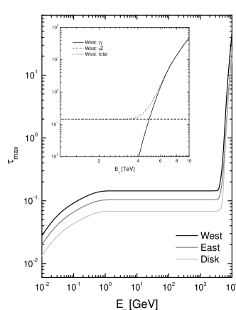
Figure 12: Opacities to $\gamma$-ray scape in the different components of Arp 220 as a function of energy. The highest energy is dominated by $\gamma\gamma$ processes, whereas $\gamma Z$ dominates the opacity at low energies. Significant $\tau_{\rm max}$ are only encountered above 1 TeV, the inset shows the total, and the contributions to the total opacity, in the case of the western nucleus of Arp 220 for this range of energy.

In Figure 12, both, the different contributions to the opacity from $\gamma\gamma$ and $\gamma Z$, in the case of the western starburst, and the total opacity for the three Arp 220 components are shown. The western nucleus is subject to the biggest opacities, its value is $\sim 0.1$ up to $\sim 4$ TeV and then rapidly increases. The equation of radiation transport (see Appendix), for the molecular disk and extreme starburst regions, are then used to compute the predicted $\gamma$-ray flux taking into account all absorption processes. The smallness of $\tau_{\rm max}$ throughout most of the energy range implies that the correction factors to the fluxes are only a few percent up to TeV energies (it is not possible to see the difference in a plot like that presented in the right panel of Figure 10). In Figure 13 the effect of TeV photon absorption in each of the components of Arp 220 is shown in detail. Note that the disk is subject to relatively lower opacities than the eastern and western extreme starbursts. This is caused mainly by a reduction of the photon target density (i.e. a reduction in $\tau^{\gamma\gamma}$ when compared with the corresponding values found in the extreme star forming regions).

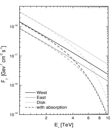
Figure 13: Fluxes with and without absorption processes being considered. Appreciable differences appear only at the highest energies.

6.6 Observability

The total predicted flux in $\gamma$-rays above 100 MeV, after the effects of absorption are taken into account at all energies, is $2.8\times 10^{-9}$ photons cm^-2 s^-1. This is comfortably below the upper limit for this galaxy imposed with EGRET data by Torres et al. (2004) in the same energy range, which is about one order of magnitude larger. It is, however, above the threshold for detection with GLAST: $F(>100\;{\rm MeV})\sim 2.4\times 10^{-9}\;{\rm photons\;cm^{-2}s^{-1}}$ is the GLAST satellite sensitivity for a 5$\sigma$ detection of a point-like, high latitude source after 1 yr of all-sky survey. If this model bears resemblance with reality, then, it might be possible for GLAST to detect Arp 220 for the first time in $\gamma$-rays.

By the same token, the total predicted fluxes in $\gamma$-rays above 300 GeV and 1 TeV are $\sim 2\times 10^{-12}$ photons cm^-2 s^-1 and $\sim 7\times 10^{-13}$ photons cm^-2 s^-1, respectively. These fluxes are high enough as to render possible, again in the case this model bears resemblance with reality, to detect Arp 220 at higher energies. Reliability of the flux predictions above 1 TeV also depends on the cross section modelling being reasonably correct.

Čherenkov telescopes cannot typically observe at zenith angles much larger than 70^∘. The zenith angle $\vartheta$ at the upper culmination of an astronomical object depends on the latitude $\phi$ of the observatory and the declination DEC of the object according to $\vartheta=|\phi-\mathrm{DEC}|$. Therefore, the condition $|\phi-\mathrm{DEC}|\leq 70^{o}$ has to be imposed in the selection of observable objects. For the next generation (but already operating) Čherenkov telescopes and because of location, Arp 220 seems to be a good candidate for a northern hemisphere observatory [e.g. MAGIC has $\vartheta\sim 5.5^{o}$; VERITAS has $\vartheta\sim 9^{o}$]. However, it seems also possible (see Petry 2001) for HESS to observe Arp 220 at high zenith angles, since DEC${}_{\rm Arp220}<+37^{o}$ implying $\vartheta<60^{o}$.

As a function of $\vartheta$, an increase in effective collection area is accompanied by a proportional increase in hadronic background rate, such that the gain in flux sensitivity is therefore only the square-root of the gain in area (Petry 2001). In addition, the higher the value of $\vartheta$, the higher is the energy threshold for observation, what reduces the integral flux. If $F_{5\sigma}(E>E_{\mathrm{thr}})$ is defined as the integral flux above the energy threshold $E_{\mathrm{thr}}$ which results in a $5\sigma$ detection after 50 h of observation time, $F_{5\sigma}(E>E_{\mathrm{thr}}(\vartheta),\vartheta)=F_{5\sigma}(E>E_{\mathrm{thr}},0^{\circ})\cdot\cos(\vartheta).$ The needed observation time to observe a source with flux $F_{5\sigma}(E>E_{\mathrm{thr}})$ can be conservatively estimated as (Petry 2001) $T_{5\sigma}(E>E_{\mathrm{thr}})=\left({F(E>E_{\mathrm{thr}})}/{F_{5\sigma}(E>E_{\mathrm{thr}})}\right)^{-2}50\,\mathrm{hours}.$ In the case of the modelling herein presented for Arp 220, assuming a generic, but conservative, $F_{5\sigma}(E>E_{300{\rm GeV}},0^{\circ})=3\times 10^{-12}$ photons cm^-2, the needed observation time for the galaxy to appear above 300 GeV is about 95 hours.

Finally, note that the decay of charged pions will also lead to the production of energetic neutrinos. While the analysis of the neutrino production and possible observability of Arp 220 by the future neutrino telescopes is left to a subsequent publication, we note that the flux of neutrinos that is outcome of this model would not violate the upper limits imposed by the AMANDA II experiment (Ahrens et al. 2004). Even if the neutrino flux from Arp 220, is the same as the photon flux, it would be below imposed upper limits to the fluxes from all candidate neutrino sources.

7 Concluding remarks

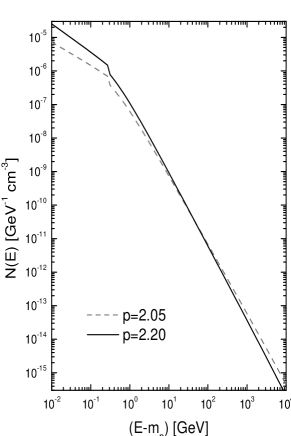
Figure 14: Left: dependence of the steady state proton distribution on the proton injection power law slope, $p$. Right: ratio between pion decay fluxes, in the western nuclei of Arp 220, for different proton injection power law slopes.

Luminous infrared galaxies are certainly interesting objects, and until recently, focus on them have been mainly granted at all wavelengths but one, the high energy domain. With several new Čerenkov telescopes, $\gamma$-ray satellites, cosmic ray, and neutrino observatories on the verge of becoming operational, or operating already, the interest on the possible high energy features of LIRGs and ULIRGs has been rekindled. There is much to learn at high energies, whether these galaxies are detected or not. Sensitivities of forthcoming equipments is –as discussed above– high enough as to impose severe constraints on theoretical models or provide interesting clues in our understanding of these objects.

Recently, ULIRGs have been analyzed as possible ultra high energy cosmic ray sources (Smialkowski, Giller & Michalak 2002; Torres & Anchordoqui 2004), and yet unidentified $\gamma$-ray detections (Torres et al. 2004; Torres 2004; Cillis et al. 2004). In this paper, a self-consistent model for the radio, IR, and $\gamma$-ray emission from Arp 220, the prototypical and nearest ULIRG, was presented. Complete agreement with observational data was obtained at all frequencies, and predictions of $\gamma$-ray fluxes were obtained. These fluxes suggest that Arp 220 could be a source for GLAST as well the new Čerenkov telescopes. The radio emission modelling of Arp 220, as the result of primary and secondary electrons’ synchrotron emission, appear to indicate that the central regions of Arp 220 are subject to a strong magnetic field.

Although many are the free parameters involved in this modelling, few are those which are unrelated to observations, and even fewer are those which –if changing– may have a significant impact on the results. Consider, as an example, the choice of the power slope for the injected proton spectrum. The model presented assumed it to be 2.2 (i.e. $Q_{\rm inj}\propto E^{-2.2}$), for all three Arp 220 components analyzed. However, there is nothing a priori yielding to this value, except that it is a reasonable and conservative expectation for the slope of a relativistic proton population in the vicinity of its acceleration site, e.g. a supernova remnant shock. But perhaps, given that the western extreme starburst is the strongest site of star formation known, the proton population might have there a harder spectrum, in particular, as compared with that found in the disk. Figure 14 explores how a change in the injected proton spectrum would affect the results. The left panel compares the steady state proton distribution for a 2.2 (the previously assumed slope) and a 2.05 spectrum. Since the same power is injected with a harder slope, the latter spectrum dominates at high energies. The right panel shows that the ratio between –for instance– $\gamma$-ray fluxes produced in pion decays in the western nucleus would not change much as a function of energy, although in the direction of favoring the possible detection.

It is also interesting to note that the electron steady distribution, interacting via inverse Compton with the abundant IR photons, will also contribute to the flux at lower frequencies, i.e. in the hard X-ray regime. Thus, a diffuse model for the high energy emission also needs to yield fluxes in agreement with imposed upper limits at hard X-ray/soft $\gamma$-ray frequencies. Dermer et al. (1997) found using OSSE that the photon flux is less than $1.2\times 10^{-4}$ photons cm^-2 s^-1, and $0.7\times 10^{-4}$ photons cm^-2 s^-1, in the 0.05–0.10 and 0.10–0.20 MeV bands, respectively. The luminosity limit in the whole energy range mentioned is $3\times 10^{43}$ erg s^-1. Iwasawa et al. (1999) found using Beppo-Sax a luminosity upper limit of $5\times 10^{40}$ and $1\times 10^{41}$ erg s^-1 in the 0.5–2 and 2–10 keV bands, respectively. These are also consistent with previously imposed ASCA limits, and stringent than those limits imposed using Chandra at such hard X-ray energies. The model discussed in this work yields inverse Compton fluxes of a few percent or less than the mentioned upper limits at these energies. Moran et al. (1999) found, although with a less detailed modelling, a similar situation in the galaxy NGC 3256. This is consistent with the hard X-ray/soft $\gamma$-ray emission being mostly generated not by diffuse processes, but by several powerful point sources, which is also the case, according to recent INTEGRAL observations (Lebrun et al. 2004), in our Galactic Center.

In closing, three remarks are deemed important to keep in mind when analyzing possible observations of Arp 220 and other LIRGs a) Additional hadronic production of high energy $\gamma$-rays with matter in the winds of stars (Romero & Torres 2003; Torres et al. 2003), and emission from particular stellar systems in general (e.g., Romero et al. 1999, Benaglia et al. 2001, Benaglia & Romero 2003) was herein disregarded, and although subdominant, it would certainly help in increasing the $\gamma$-ray emission at the highest energies. b) Only non-variable $\gamma$-ray sources can be ascribed to LIGs if diffusive process such as the one explored in this work are responsible for the emission. Variability indices (Torres et al. 2001, Nolan et al. 2003) could then help in discriminating unidentified detections. c) The small redshift of Arp 220 and other galaxies in the 100 Mpc sphere makes opacities due to processes with photons of the cosmic microwave and IR background outside the galaxy negligible below 10 TeV (see, e.g., figure 2 of Aharonian 2001).

Acknowledgements

This work was performed under the auspices of the U.S. D.O.E. (NNSA) by the University of California Lawrence Livermore National Laboratory, under contract No. W-7405-Eng-48. I thank Felix Aharonian, Luis Anchordoqui, Steve Blattnig, Valenti Bosch-Ramón, Analia Cillis, Thomas Dame, Seth Digel, Eva Domingo-Santamaría, Yu Gao, Felix Mirabel, Martin Pessah, Olaf Reimer, Gustavo Romero, Nick Scoville, & Wil Van Breugel for comments related to this work. Eva Domingo, Seth Digel, and Analia Cillis are further thanked for discussions on TeV analysis of data, GLAST sensitivity, and EGRET upper limits, respectively. Martin Pessah is further acknowledged for discussions regarding geometry. An anonymous referee is also acknowledged. I finally thank Ileana Andruchow for support.

Appendix

Here we present some of the main formulae used in the paper and a few details of implementation. For a more complete account see the SPIRES-HEP version (astro-ph/0407240) of this article.

Proton losses

During the motion of a proton through a neutral medium, the ionization loss rate is given by (e.g., Ginzburg & Syrovatskii 1964, p.120ff)

$$-\left(\frac{dE}{dt}\right)_{{\rm Ion},p}\sim 1.83\times 10^{-17}\left(\frac{n_{\rm H}+2n_{{{\rm H}}_{2}}}{{\rm cm}^{-3}}\right)\frac{c}{v}\left\{10.9+2\ln\left(\frac{E}{m_{p}c^{2}}\right)+\ln\left(\frac{v^{2}}{c^{2}}\right)-\frac{v^{2}}{c^{2}}\right\}{\rm GeV\;s}^{-1}.$$ (14)

The energy loss by pion production is given as (Mannheim and Schlickeiser 1994, Schlickeiser 2002, p. 125 and 138)

$$-\left(\frac{dE}{dt}\right)_{{\rm Pion},p}\sim 5.85\times 10^{-16}\,\left(\frac{n}{{\rm cm}^{-3}}\right)\,\left(\frac{E_{p}-m_{p}c^{2}}{\rm GeV}\right)\,\Theta(E_{p}-E_{\rm th})\,{\rm GeV\;s}^{-1}.$$ (15)

Electron losses

In the ultrarelativistic case ($E\gg mc^{2}$), the ionization losses in neutral atomic matter (e.g., Schlickeiser 2002, p. 99; Ginzburg & Syrovatskii 1964, p. 140ff)

$$-\left(\frac{dE}{dt}\right)_{{\rm Ion},e}\sim 2.75\times 10^{-17}\left[6.85+\ln\left(\frac{E}{mc^{2}}\right)\right]\left[\frac{n_{\rm H}+2n_{{{\rm H}}_{2}}}{{\rm cm}^{-3}}\right]{\rm GeV\,s}^{-1}.$$ (16)

Synchrotron losses can be computed as (e.g., Ginzburg & Syrovatskii 1964, p. 145ff; Blumenthal & Gould 1970)

$$-\left(\frac{dE}{dt}\right)_{{\rm Sync},e}=\frac{2}{3}c\left(\frac{e^{2}}{mc^{2}}\right)^{2}B_{\bot}^{2}\left(\frac{E}{mc^{2}}\right)^{2}\sim 2.5\times 10^{-6}\left(\frac{B}{{\rm Gauss}}\right)^{2}\left(\frac{E}{{\rm GeV}}\right)^{2}{\rm GeV\;s}^{-1},$$ (17)

where $B_{\bot}$ represents the magnetic field in a direction perpendicular to the electron velocity, and the second equality takes into account that an isotropic distribution of pitch angles. In this case, particles velocities are distributed according to $p(\alpha)d\alpha=[(1/2)\sin\alpha)]d\alpha$, with $\alpha$ the angle between the particle’s velocity and $B$, varying between 0 and $\pi$. Then, as $B_{\bot}=B\sin\alpha$, the average in Eq. (17) requires the integral $\int[(1/2)\sin\alpha)]\sin^{2}\alpha\,d\alpha=2/3$, in order to go from $B_{\bot}$ to $B$.

The losses produced by Inverse Compton emission are given by (e.g., Blumenthal & Gould 1970)

$$-\left(\frac{dE}{dt}\right)_{{\rm IC},e}=\int_{0}^{\infty}d\epsilon\,\int_{{E_{\gamma}}^{\rm min}}^{{E_{\gamma}}^{\rm max}}\,dE_{\gamma}\,E_{\gamma}c\,n_{\rm ph}(\epsilon)\,\frac{d\sigma(\epsilon,E_{\gamma},E)}{dE_{\gamma}}$$ (18)

where $n_{\rm ph}(\epsilon)$ is the target photon distribution (usually a black or a greybody), $\epsilon$ and $E_{\gamma}$ are the photon energies before and after the Compton collision, respectively, and $d\sigma(\epsilon,E_{\gamma},E)/dE_{\gamma}$ is the Klein-Nishina differential cross section (Schlikeiser 2002, p. 82).

Additional losses are caused by the emission of bremsstrahlung $\gamma$-ray quanta in interactions between electrons and atoms of the medium. The energy loss can be computed as (e.g., Schlickeiser 2002, p. 95ff; Ginzburg & Syrovatskii 1964, p. 143, Blumenthal & Gould 1970):

$$-\left(\frac{dE}{dt}\right)_{{\rm Brem},e}=\int dE_{\gamma}\;E_{\gamma}\left(\frac{dN}{dt\,dE_{\gamma}}\right),$$ (19)

where $({dN}/{dt\,dE_{\gamma}})=c\sum_{j}n_{j}(d\sigma_{j}/dE_{\gamma})$ represents the number of photons emitted with energy $E_{\gamma}$ by a single electron of initial energy $E$ in a medium with $j$ different species of corresponding densities $n_{j}$, and where $(d\sigma_{j}/dE_{\gamma})$ is the Bethe-Heitler differential cross section.

Leptonically-generated high energy radiation

The bremsstrahlung emissivity can be computed from the steady CR electron spectrum as the integral as ${Q_{\gamma}(E_{\gamma})}_{{\rm Brem}}=n\,{E_{\gamma}}^{-1}\int_{{E_{\gamma}}}^{\infty}dE_{e}\,c\,N_{e}(E_{e})\,\sigma_{{\rm Brem}},$ where $\sigma_{{\rm Brem}}$ is the bremsstrahlung cross section, equal to $3.38\times 10^{-26}$ cm², and $n=(n_{\rm H}+2n_{{{\rm H}}_{2}})$ is the ISM atomic hydrogen density.

The inverse Compton emissivity is given by

$${Q_{\gamma}(E_{\gamma})}_{{\rm IC}}=\int_{0}^{\infty}n_{\rm ph}(\epsilon)d\epsilon\int_{E_{\rm min}}^{E_{\rm max}}\frac{d\sigma(E_{\gamma},\epsilon,E_{e})}{dE_{\gamma}}\,c\,N_{e}(E_{e})dE_{e}\;.$$ (20)

${E_{\rm max}}$ is the maximum electron energy for which the distribution $N_{e}(E_{e})$ is valid. ${E_{\rm min}}$ is the minimum electron energy needed to generate a photon of energy $E_{\gamma}$, i.e. ${E_{\rm min}}=(E_{\gamma}/2)[1+(1+(mc^{2})^{2}/\epsilon E_{\gamma})^{1/2}]$.

Synchrotron emission

The synchrotron emissivity can be written as

$$\epsilon_{\rm Sync}(\nu)=1.166\times 10^{-20}\left(\frac{B}{\rm Gauss}\right)\int dE\,N(E){\int_{0}}^{\pi/2}d\alpha\,\frac{\nu}{\nu_{c}}\sin^{2}\alpha\int_{\nu/\nu_{c}}^{\infty}d\xi K_{5/3}(\xi)\;$$

$$\hskip 142.26378pt{\rm GeV\,s^{-1}\,cm^{-3}\,Hz^{-1}\,sr^{-1}}.$$ (21)

A useful result is given by the product of $\epsilon_{\rm Sync}$ and $V/D^{2}$, $f_{\rm Sync}(\nu)$. This is the synchrotron flux density (units of Jy) expected from a region of volume $V$ located at a distance $D$ in cases in which opacities are negligible, see below. In cases where opacities are not negligible, one has to solve first for the specific intensity considering all absorption processes, compute the emissivity, and consider the geometry.

Free-free emission and absorption

The emission and absorbtion coefficients for this process are given by the following expressions (e.g., Rybicki & Lightman 1979, Ch. 5, Schlickeiser 2002, Ch. 6) $\epsilon_{\rm ff}(\nu)=3.37\times 10^{-36}Z^{2}\left({n_{e}n_{i}}/{\rm cm^{-6}}\right)\left({T}/{\rm K}\right)^{-1/2}\left({\nu}/{\rm GHz}\right)^{-0.1}e^{-h\nu/kT}{\rm GeV\,cm^{-3}\,s^{-1}\,Hz^{-1}\,sr^{-1}}$ and $\kappa_{\rm ff}(\nu)=2.665\times 10^{-20}Z^{2}\left({T}/{\rm K}\right)^{-1.35}\left({n_{e}n_{i}}/{\rm cm^{-6}}\right)\left({\nu}/{\rm GHz}\right)^{-2.1}{\rm cm^{-1}},$ respectively. Here, the plasma is described by a temperature $T$, metallicity $Z$ and thermal electron and ion densities $n_{e}$ and $n_{i}$, respectively. The free-free opacity is given by the integral $\tau_{\rm ff}\equiv\int_{0}^{\infty}dr\,\kappa_{\rm ff}\sim 8.235\times 10^{-2}\left({T}/{\rm K}\right)^{-1.35}\left({\nu}/{\rm GHz}\right)^{-2.1}\left({\rm EM}/{\rm cm^{-6}\,pc}\right),$ where EM is the emission measure, defined as EM=$\int_{0}^{\infty}dr\,n_{i}n_{e}$. For simplicity, and in lack of other knowledge, it is assumed that the EM is constant. The turnover frequency $\nu_{t}$ (for frequencies less than $\nu_{t}$ the emission is optically thick) can also be given in terms of EM, $\nu_{t}=0.3[({T}/{\rm K})^{-1.35}{\rm EM}]^{1/2}$ GHz.

Radiation transport equation, and fluxes from emissivities

This paper analyzes the case in which emission and absorption are uniform, co-spatial, and without further background or foreground sources or sinks (see, e.g., Appendix A in Schlickeiser 2002). The solution to the radiation transport equation in these situations is $I_{\nu}=\frac{\epsilon_{\nu}}{\kappa_{\nu}}(1-e^{-\tau_{\nu}}),$ where $\epsilon_{\nu}$ is the emission coefficient –or emissivity–, $\kappa_{\nu}$ is the absorption coefficient, and $\tau_{\nu}=\kappa_{\nu}L$ is the opacity in the far end ($L$) of the emission region (also referred to as the maximum opacity). In cases in which there are more than one process involved in the emission or in the absorption, a sum over processes must be performed. Units are consistent with the rest of the paper, such that $[\epsilon_{\nu}]=$ GeV cm^-3 s^-1 sr^-1 Hz^-1 (in the case of $\gamma$-rays, photon emissivities are used instead, $Q/4\pi$, with units of photons cm^-3 s^-1 sr^-1 GeV^-1), $[\kappa_{\nu}]=$cm^-1, and $[\tau]=1$. Additionally, $I_{\nu}$ is the emergent intensity ($[I_{\nu}]=$GeV cm^-2 s^-1 sr^-1) after the absorption processes are considered.

Consider first the case in which opacities are negligible. To compute the flux, given the knowledge of its emissivity under a particular process, information on the solid angle -as seen from the observer- ($\Omega$) and depth ($L$) along the line of sight, or volume and distance of the region of emission is needed. For instance, the integral flux of $\gamma$-rays, with no absorption, is given by

$$F_{\gamma}(E_{\gamma}>E)=\int_{E}^{\infty}{Q_{\gamma}(E_{\gamma})}\frac{\left[\Omega L\right]_{\rm obs}}{4\pi}dE_{\gamma}=\frac{V}{4\pi D^{2}}\int_{E}^{\infty}{Q_{\gamma}(E_{\gamma})}dE_{\gamma},$$ (22)

where ${Q_{\gamma}(E_{\gamma})}={Q_{\gamma}(E_{\gamma})}_{{\rm Brem}}+{Q_{\gamma}(E_{\gamma})}_{{\rm IC}}+{Q_{\gamma}(E_{\gamma})}_{\pi^{0}}$ is the total $\gamma$-ray emissivity, and ${\left[\Omega L\right]_{\rm obs}}/{4\pi}$ corrects for the fraction of the emission which is in the direction of the observer. Clearly, in this case, the differential photon flux is $F_{\gamma}(E_{\gamma})=[{V}/{4\pi D^{2}}]{Q_{\gamma}(E_{\gamma})}$.

When there are absorption processes involved, but the geometry is such that $I$ is not depending on the position within the emitting region, i.e., when both emission and absorption coefficients are uniform and the maximum value of $\tau$ is the same for all the region, the flux can be computed as

$$F_{\nu}=\frac{\epsilon_{\nu}}{\tau_{\nu}}(1-e^{-\tau_{\nu}})\frac{V}{D^{2}}\equiv\epsilon_{\nu}\frac{V}{D^{2}}f_{1}.$$ (23)

However, in the case of an sphere, for example, even when emission and absorption are uniform, the specific intensity is not. Because the linear size is different at different angles $\theta^{\prime}$ as measured from the center of the sphere, the opacity will also change. This change can be represented as $\tau_{\nu}=\kappa_{\nu}\times 2R\cos\theta^{\prime}=\tau_{\rm max}\cos\theta^{\prime}$, i.e. through the use of the maximum opacity $\tau_{\rm max}$ affecting a photon equatorially traversing the system. $\tau_{\rm max}$ is also a function of the frequency, although the subindex $\nu$ is omitted for simplicity. The flux is

$$F = \int I[\cos\theta]\ d\Omega=\int\frac{\epsilon_{\nu}}{\kappa_{\nu}}(1-e^{{-\tau_{\nu}}(\theta^{\prime})})\,2\pi\,\cos\theta\,\sin\theta\,d\theta$$ (24)

$$= \frac{\epsilon_{\nu}}{\kappa_{\nu}}2\pi\int_{0}^{\theta_{\rm max}}\left(1-e^{\tau_{\rm max}\sqrt{1-(D/R)^{2}\sin\theta}}\right)\cos\theta\sin\theta d\theta.$$

The solution to this integral can be analytically obtained and after some algebra the result can be written as

$$F=\frac{\epsilon_{\nu}}{\tau_{\rm max}}\frac{V}{D^{2}}\left[\frac{3}{2}+\frac{3}{\tau_{\rm max}^{2}}\left((1+\tau_{\rm max})e^{-\tau_{\rm max}}-1\right)\right]\equiv\epsilon_{\nu}\frac{V}{D^{2}}f_{2}.$$ (25)

Note that when $\tau_{\rm max}\ll 1$ the previous result reduces to the case of no absorption, $f_{2}=1$. Figure 15 shows the behavior of the correction factors for absorption that appear in the different contexts analyzed in this paper, $f_{1}$ and $f_{2}$.

Figure 15: Correction factors for absorption. The $f_{2}/f_{1}$ curve asymptotically tends to 1.5.

Dust emission

We assume that the dust photon emissivity, which dominates the luminosity at micron-frequencies, is given by $q_{d}=q_{0}\epsilon^{\sigma}B(\epsilon,T)$, where $\sigma\sim 1-2$ is the emissivity index, $B(\epsilon,T)$ is the Planck function of temperature $T$, and $\epsilon$ is the photon energy (see, e.g., Rice et al. 1988; Goldshmidt and Rephaeli 1995; Krügel 2003, p.245). Units correspond to $[q_{d}]=$ photons s^-1 cm^-2. Then, the flux produced by dust can be computed as $F=2\pi\int_{0}^{\pi/2}q_{d}\cos\theta\sin\theta d\theta d\epsilon=\pi\int q_{d}d\epsilon$ and normalized to $[L/4\pi R^{2}]$, with $L$ and $R$ being the IR luminosity and radius of the emitting region, respectively; i.e., normalized to the power per unit area through the surface of the emitting region. This fixes the dimensional constant. Units are such that $[q_{0}]=$ GeV^-1-σ s^-1, and [$B(\epsilon,T)]=$ GeV cm^-2.

The flux density of dust emission at the surface of the emitting region is obtained from the definition $F\equiv\int f_{\rm dust}(\nu)d\nu$, where units are, for consistency, $[f_{\rm dust}]=$ s^-1 cm^-2 Hz^-1 GeV. The IR photon number density per unit energy, $n(\epsilon)$, can be obtained by equating the particle flux outgoing the emission region, $\pi R^{2}cn(\epsilon)\epsilon d\epsilon$, with the expression of the same quantity that make use of the emissivity law, $4\pi R^{2}\pi q(\epsilon)d\epsilon$.

References

- (1) Aharonian F. A., Drury L. O’C., & Völk H. J. 1994, A&A 285, 645
- (2) Aharonian F. A. & Atoyan, A. M. 1996, A&A 309, 91
- (3) Aharonian F. A. 2001, Rapporteur, and Highlight papers of ICRC 2001: 250
- (4) Ahrens J., et al. 2004, Phys. Rev. Lett. 92, 071102
- (5) Atoyan A. M., Aharonian F. A. & Völk H. J. 1995, Physical Review D52, 3255
- (6) Abraham P. B., Brunstein K. A. & Cline T. L. 1966, Physical Review 150, 150
- (7) Baan W. A., Wood P. A. D. & Haschick A. D. 1982, ApJ 260, L49
- (8) Baan W. A. & Haschick A. D. 1995, ApJ 454, 745
- (9) Bhabha H. J. 1938, Proc. Roy. Soc. (London) A164, 258
- (10) Badhwar G. D., Stephens S. A. & Golden R. L. 1977, Physical Review D15, 820
- (11) Beck R. 2001, Space Science Reviews 99, 243
- (12) Bell A. R. 1978, MNRAS 182, 443
- (13) Benaglia P., Romero G. E., Stevens I. R. & Torres D. F. 2001, A&A 366, 605
- (14) Benaglia P. & Romero G. E. 2003, A&A 399, 1121
- (15) Blattnig S. R. et al. 2000a, Physical Review D62, 094030
- (16) Blattnig S. R. et al. 2000b, NASA/TP-2000-210640, Langley Research Center, available online at http://techreports.larc.nasa.gov/ltrs/PDF/2000/tp/NASA2000tp210640.pdf
- (17) Blom J. J., Paglione T. A. & Carramiñana A. 1999, 516, 744
- (18) Brogan C. L., Frail D. A., Goss W. M. & Troland T. H. 2000, ApJ 537, 875
- (19) Brown R. L. & Marscher A. P. 1977, ApJ 212, 659
- (20) Bryant P. M., & Scoville N. Z. 1999, ApJ 117, 2632
- (21) Carico D. P., Keene J., Soifer B.T. & Neugebauer G. 1992, PASP 104, 1086
- (22) Chevalier R. A. 1982, ApJ 259, 302
- (23) Cillis A., Torres D. F. & Reimer O. 2004, in preparation
- (24) Clements D. L., MacDowell J. C., Shaked S., Baker A. C., Borne K., Collina L., Lamb S., Mundell S., 2002, ApJ, 581, 974
- (25) Condon J. J., Huang Z. P., Yin Q. F. & Thuan T. X. 1991, ApJ 378, 65
- (26) Cox, A. N. 1999, Allen’s Astrophysical Quantities, Springer Verlag, New York
- (27) De Gouveia Dal Pino E. & Medina Tanco G. A. 1999, ApJ 518, 129
- (28) Dermer C. D., & Schlickeiser R. 1991, A&A 252, 414
- (29) Dermer C. D., Bland-Hathworn J., Chiang J. & McNaron-Brown K. 1997, ApJ 484, L121
- (30) Domingo-Santamaria E. & Torres D. F. , arXiv:astro-ph/0506240. To appear in A&A.
- (31) Donahue T.M. 1951, Physical Review 84, 972
- (32) Downes D., & Solomon P.M. 1998, ApJ 507, 615
- (33) Downes D., Solomon P. M. & Radford S. J. E. 1993, ApJ 414, L13
- (34) Drury L. O’C., Aharonian F. A. & Völk H. J. 1994, A&A 287, 959
- (35) Duric N., Gordon S. M., Goss W. M., Viallefond F. & Lacey C. 1995, ApJ 445, 173
- (36) Eales S. A., Wynn-Williams C. G. & Duncan W. D. 1989, ApJ 339, 859
- (37) Ellison D. C., Decourchelle A. & Ballet J. 2004, A&A 413, 189
- (38) Fazio G. G. 1967, ARA&A 5, 481
- (39) Fatuzzo M. & Melia F. 2003, ApJ 596, 1035
- (40) Feenberg E. & Primakoff H. 1948, Physical Review 73, 449
- (41) Gaisser T. K. 1990, Cosmic Rays and Particle Physics, Cambridge University Press, Cambridge, UK
- (42) Gao Y. & Solomon P. M. 2004a, ApJ Suppl. 152, 63
- (43) Gao Y. & Solomon P. M. 2004b, ApJ 606, 271
- (44) Ginzburg V. L. & Syrovatskii S. I. 1964, “The origin of cosmic rays”, Pergamon Press, Oxford, England.
- (45) Gonzalez-Alfonso E., Smith H. A., Fischer J. & Cernicharo J. 2004, astro-ph/0406427
- (46) Hummel E. & Beck R. 1995, A&A 303, 691
- (47) Iwasawa K., Matt G., Guainazzi M. & Fabian A. C. 2001, MNRAS 326, 894
- (48) Killeen N. 1996, et al. MNRAS 280, 1143
- (49) Koralesky B., Frail D. A., Goss W. M., Claussen M. J. & Green, A. J. 1998, AJ 116, 1323
- (50) Krügel E. 2003, “The physics of interestellar dust”, IoP, Cambridge
- (51) Lebrun F. et al. 2004, Nature 428, 293
- (52) Longair M. S. 1994, “High Energy Astrophysics, Vol.2: Stars, the Galaxy and the Interstellar Medium”, Cambridge University Press, 2nd ed.
- (53) Lonsdale C. J., Diamond P.J., Smith H. E. & Lonsdale C. J. 1998, ApJ 493, L13
- (54) Lonsdale C. J., et al. 2001, in Galaxies and their Constituents at the Highest Angular Resolutions, Proceedings of IAU Symposium 205, held 15-18 August 2000 at Manchester, United Kingdom. Edited by R. T. Schilizzi, 2001, p. 386
- (55) Mannheim K. & Schlickeiser R. 1994, A&A 286, 983
- (56) Manucci F. et al. 2003, A&A 401, 519
- (57) Maraschi L., Perola G. C. & Schwarz S. 1968, Il Nuovo Cimento LIII B, 1975
- (58) Markoff S., Melia, F. & Sarcevic I. 1999, ApJ 522, 870
- (59) Marscher A. P. & Brown R. L. 1978, ApJ 221, 588
- (60) Mattila S. & Meikle W. P. S. 2001, MNRAS 324, 325
- (61) Mirabel F. & Sanders D. B. 1989, ApJ 335, 104
- (62) Mirabel F. & Sanders D. B. 1989, ApJ 340, L53
- (63) Morfill G. E. 1982, ApJ 262, 749
- (64) Moran E. C., Lehnert M. D. & Helfand D. J. 1999, ApJ 526, 649
- (65) Moskalenko I. & Strong A. 1998, ApJ 493, 694
- (66) Nolan P., Tompkins W., Grenier I. & Michelson P. 2003, ApJ, 597, 615
- (67) Orth C. D. & Buffington A. 1976, ApJ 206, 312
- (68) Padmanabhan T. 2000, “Theoretical Astrophysics, Vol. I”, Cambridge University Press, Cambridge, UK
- (69) Paglione T. A. D., Marscher A. P., Jackson J. M. & Bertsch D. L. 1996, ApJ 460, 295
- (70) Petry D. 2001, Proc. Int. Workshop on The Nature of Galactic Unidentified Gamma-ray Sources, O. Carramiñana, O. Reimer, D. Thomson Eds., Kluwer Academic Press, p.299
- (71) Plante R. L., Lo K. Y., Crutcher R. M. & Killeen, N. E. B. 1994, in The Magnetic Field at the Galactic Center: Detection of HI Zeeman Splitting, in R. Genzel and A. I. Harris (eds.), The Nuclei of Normal Galaxies, Kluwer Acad. Publ., Dordrecht, p. 205207.
- (72) Ramaty R., Lingenfelter R. E. 1966, Journal of Geophysical Research 71, 3687
- (73) Reich W. 1994, in R. Genzel and A. I. Harris (eds.), The Nuclei of Normal Galaxies, Kluwer Acad. Publ., Dordrecht, p. 5562
- (74) Rieke G. 1988, ApJ 331, L5
- (75) Rigopoulou D., Lawrence A. & Rowan-Robinson M. 1996, MNRAS 278, 1049
- (76) Rodriguez-Espinosa J. M., Perez-Garcia A. M., Lemke D. & Meisenheimer K. 1996, A&A 315, L129
- (77) Romero G. E., Benaglia P. & Torres D. F. 1999, A&A 348, 868
- (78) Romero G. E. & Torres D. F. 2003, ApJ 586, L33
- (79) Rovilos et al. 2002, 6th European VLBI Network Symposium on New Developments in VLBI Science and Technology, held in Bonn, June 25th-28th 2002, proceedings edited by E. Ros, R. W. Porcas, A. P. Lobanov, and J. A. Zensus, published by the Max-Planck-Institut fuer Radioastronomie (Bonn). p. 179.
- (80) Rovilos et al. 2003, MNRAS 342, 373
- (81) Sakamoto K., Scoville N. Z., Yun M. S., Crosas M., Genzel R. & Tacconi L. J. 1999, ApJ 514, 688
- (82) Sanders D. B. & Mirabel I. F. 1996, ARA&A 34, 749
- (83) Schlickeiser R. 1982, A&A 106, L5
- (84) Schlickeiser R. 2002, “Cosmic ray astrophysics”, Springer-Verlag, New York
- (85) Scoville N. Z., Sargent A. I., Sanders D. B. & Soifer B. T. 1991, ApJ 366, L5
- (86) Scoville N. Z., Yun M. S. & Bryant P. M. 1997, ApJ 484, 702
- (87) Shioya Y., Trentham N. & Taniguchi Y. 2001, ApJ 548, L29
- (88) Smialkowski A., Giller M. & Michalak W. 2002, J. Phys. G 28, 1359
- (89) Smith H. E., Lonsdale C. J., Lonsdale C.J. & Diamond P.J. 1998, ApJ 493, L17
- (90) Smith H. E., Lonsdale C. J., Lonsdale C.J. & Diamond P.J. 1998b, ApJ 492, 137
- (91) Soifer B. T., et al. 1999, ApJ 513, 207
- (92) Sopp H. M. & Alexander P. 1991, MNRAS 251, 112
- (93) Stecker F. W. 1969, Astrophysics and Space Science 6, 377
- (94) Stecker F. W. 1972, Astrophysics and Space Science 20, 47
- (95) Stecker F. W. 1977, ApJ 212, 60
- (96) Stephens S. A. & Badhwar G. D. 1981, Astrophysics and Space Science 76, 213
- (97) Strong A. & Moskalenko I. 1998, ApJ 509, 212
- (98) Torres D. F., Romero G. E., Combi J. A., Benaglia P., Andernach H. & Punsly B. 2001, A&A 370, 468
- (99) Torres D. F., Romero G. E., Dame T. M., Combi J. A. & Butt Y. M. 2003, Physics Reports 382, 303
- (100) Torres D. F., Domingo-Santamaría E., & Romero G. E. 2003, ApJ 601, L75
- (101) Torres D. F. 2004, in Cosmic Gamma-ray Sources, edited by K. S. Cheng and G. E. Romero, Kluwer Academic Press, in press. arXiv:astro-ph/0308069.
- (102) Torres D. F., Reimer O., Domingo-Santamaría E. & Digel S. 2004, ApJ 607, L99
- (103) Torres D. F. & Anchordoqui L. A. 2004, Report on Progress in Physics, in press, arXiv:astro-ph/0402371.
- (104) Uchida K. I. & and Güsten R. 1995, A& 298, 473
- (105) Van Buren D. & Greenhouse M. 1994, ApJ 431, 640
- (106) Völk H. J., Klien U. & Wielebinski R. 1989, A&A 237, 21
- (107) Wiedner M. C., Wilson C. D., Harrison A., Hills R. E. & Carlstrom J. E. 2002, ApJ 581, 229
- (108) Woody D. P., et al. 1989, ApJ 337, L41
- (109) Yao L., Seaquist E.R., Kuno N. & Dunne L. 2003, ApJ 588, 771
- (110) Yusef-Zadeh F., Roberts D. A., Goss W. M., Frail D. A. & Green A. J. 1996, ApJ 466, L25