Scale sensitive deconvolution of interferometric images

Deconvolution of the telescope Point Spread Function (PSF) is necessary for even moderate dynamic range imaging with interferometric telescopes. The process of deconvolution can be treated as a search for a model image such that the residual image is consistent with the noise model. For any search algorithm, a parameterized function representing the model such that it fundamentally separates signal from noise will give optimal results. In this paper, the first in a series of forthcoming papers, we argue that in general, spatial correlation length (a measure of the scale of emission) is a stronger separator of the signal from the noise, compared to the strength of the signal alone. Consequently scale sensitive deconvolution algorithms result into more noise-like residuals. We present a scale-sensitive deconvolution algorithm for radio interferometric images, which models the image as a collection of Adaptive Scale Pixels (Asp). Some attempts at optimizing the runtime performance are also presented.

1 Introduction

Interferometric telescopes employ the van Cittert-Zernike theorem to synthesize apertures much larger than the size of the individual antennas (Thompson et al. 2001). Such instruments measure the source coherence function, which is the Fourier transform of the sky brightness distribution. However the source coherence function is measured at discrete points in the Fourier space resulting into a point spread function (PSF) which has significant wide-spread sidelobes. The presence of these sidelobes limits the dynamic range of raw images made with such telescopes. For even moderate dynamic range imaging, deconvolution of the PSF is necessary.

The measurement equation describing an interferometer can be written as:

$$\@vec{V}=\@tens{A}\@vec{I^{o}}+\@tens{A}\@vec{N}$$ (1)

where $\@vec{V}$ and $\@vec{N}$ are the measured visibility and independent random noise vectors respectively, and $\@vec{I^{o}}$ is the true image. The measurement matrix $\@tens{A}$ represents the linear transform from the image to the visibility domain. For perfectly calibrated co-planar Fourier synthesis devices like imaging interferometric telescopes, $\@tens{A}$ is the rectangular observation matrix, the non-zero elements of which are the sines and cosines corresponding to the measured fourier components. In practice, due to incomplete sampling of the visibility domain, $\@tens{A}$ in general is a singular non-square matrix, excluding the use of linear methods to invert the above equation. Non-linear deconvolution methods are therefore used to estimate $\@vec{I^{o}}$. In the usual terminology used in the literature, $\@tens{A}^{\rm T}\@vec{V}$ is the dirty image ($\@vec{I^{d}}$) and $\@tens{A}^{\rm T}\@tens{A}=\@tens{B}$ is the beam matrix (the super-script $\rm T$ implies a transpose). $\@tens{B}$ is a toeplitz matrix of the dirty beam or the point spread function and $\@tens{B}\@vec{I^{o}}$ represents the convolution of the true image with the PSF. Note that the resultant noise vector in the image domain ($\@tens{A}^{\rm T}\@tens{A}\@vec{N}$) is also convolved with the PSF and the pixel-to-pixel noise in the image is not independent.

The process of deconvolution can be described as a search for a model image $\@vec{I^{M}}$ which solves the normal equation

$$\@tens{A}^{\rm T}\@vec{V}=\@tens{A}^{\rm T}\@tens{A}\@vec{I^{M}}+\@tens{A}^{\rm T}\@tens{A}\@vec{N}$$ (2)

A non-linear minimization scheme can be set up which iteratively minimizes the objective function until the residuals $\@vec{V}-\@tens{A}\@vec{I^{M}}$ are noise-like.

The dimensionality and the nature of the search space is governed by the parameterization of $\@vec{I^{M}}$. Scale insensitive deconvolution algorithms like CLEAN (Högbom 1974) and its variants model the image as

$$\@vec{I^{M}}=\sum_{k}F_{k}\delta(x-x_{k},y-y_{k})$$ (3)

which is a collection of delta functions of amplitude $F_{k}$ at each pixel location. An $N\times M$ pixel clean-box corresponds to a $N\times M$ dimensional search space. The CLEAN algorithm iteratively estimates the $F_{k}$s by taking a fixed sized step along the axis of highest derivative (the peak in the residual image) (see Schwarz 1978, for a more complete description). This is done by updating the residual image at each iteration as $\@vec{I}^{\@vec{R}}_{k}=\@vec{I}^{\@vec{R}}_{k-1}-g\@tens{B}\left[\max{\@vec{I}^{\@vec{R}}_{k-1}}\right]$ where $g$ is called the loop-gain (it controls the step-size). This implicitly assumes an orthogonal search space of constant curvature. Variants of CLEAN (Clark 1980) operate in two cycles called major and minor cycles. The minor cycle uses an approximate PSF and builds a shallow model image. The accuracy lost in the minor cycle due to the use of approximate PSF is recovered in the more expensive major cycle where the residual image is computed at full accuracy as $\@tens{A}^{\rm T}\left[\@vec{V}-\@tens{A}\@vec{I^{M}}\right]$. It can therefore be considered to be a steepest descent algorithm to minimize the objective function $\chi^{2}=\left[\@vec{V}-\@tens{A}\@vec{I^{M}}\right]^{\rm T}\@tens{W}\left[\@vec{V}-\@tens{A}\@vec{I^{M}}\right]$. The dimensionality of the search space can be constrained by the user defined clean-box which usually remains fixed after initial specification. The step size is also a user defined parameter, typically $\leq 0.2$. The stopping criterion is a combination of the maximum number of iterations and the magnitude of the maximum residual. Typically, the algorithm is stopped (often by user intervention or by adjusting the maximum number of iterations) when maximum residuals are comparable to the estimated noise (another user defined parameter). The regularization to avoid the problem of over fitting in such an unconstrained minimization is explicitly imposed via forcing a finite number of iterations.

Statistical image reconstruction algorithms like Maximum Entropy Method (MEM) (Narayan & Nityananda 1986, and references therein) on the other hand set up a formal constrained minimization algorithm which minimizes the objective function $f(\@vec{I^{M}},\lambda)=H-\lambda\chi^{2}$ where $H$ is the entropy function, $\lambda$ is a Lagrange multiplier and the model image is parameterized as in Eq. 3. The function $H$ is derived from a physically meaningful prior distribution and imposes various desirable constraints like smoothness. An extra term, sometimes with another undetermined Lagrange multiplier is also used to impose the positivity constraint. The Entropy function acts as a regularizer, biasing the solution towards the supplied prior image while $\chi^{2}$ pulls the solution towards the best fit to the data. From a set of images all of which satisfy the normal equation (Eq. 2), the MEM image corresponds to the mode of the a-posterior distribution. The step size computation for the minimization of $f$ requires an evaluation of the inverse of the Hessian matrix. For images with a large number of pixels with significant emission, the size of the Hessian matrix can be large and inverting it typically requires SVD like algorithms which are computationally expensive. Cornwell & Evans (1985) devised a fast iterative algorithm by approximating the Hessian by a diagonal matrix to gain in speed.

Both approaches however use the parameterization in Eq. 3 which we refer to as a scale-less model. The image is decomposed into a set of delta functions and the search space is assumed to be orthogonal.

Coupling of the pixels in the dirty image comes from two sources. The pixels of the underlying true image are inherently not independent in the presence of extended emission. The second source of coupling comes from the PSF. As mentioned earlier, the main lobe of the PSF has a finite width (proportional to the diffraction limit of the synthesized aperture) and significant wide-spread sidelobes. The former kind of coupling implies that the search space is potentially non-orthogonal unless the true sky is composed only of clearly unresolved sources. The latter however implies a coupling of even widely separated unresolved sources via the sidelobes of the PSF. Ignoring the coupling due to the PSF possibly only results into slower convergence. However, ignoring the inherent coupling of pixels for extended emission allows more degrees of freedom (DOF) than required, which results into the breaking up of the extended emission leaving low level correlated residuals. The peak residuals are comparable to the estimated noise but are correlated at scales larger than the resolution element (the synthesized beam). In the absence of any scale information in Eq. 3, such residual emission cannot be recovered.

It is easy to see that an optimal image reconstruction algorithm will also use the minimum number of DOF to represent the image. However in practice, it is almost impossible to determine this minimum number, and hence also difficult to design an algorithm which will achieve such a representation Practically therefore, the goal is to seek a solution with least complexity. From the point of view of imaging weak extended emission, the important improvement in the deconvolution algorithm is therefore to decompose the true sky image in a scale sensitive basis. This implies a significant increase in algorithm complexity and computational cost. In this paper we describe a scale sensitive deconvolution algorithm for interferometric images and attempts at improving its performance.

2 Fundamental separation of signal and noise

Equation 2 can be written in terms of the dirty and true images as

$$\@vec{I^{d}}=\@tens{B}\@vec{I^{o}}+\@vec{I^{N}}\leavevmode\nobreak\ \leavevmode\nobreak\ \leavevmode\nobreak\ \leavevmode\nobreak\ {\rm where}\leavevmode\nobreak\ \leavevmode\nobreak\ \leavevmode\nobreak\ \@vec{I^{N}}=\@tens{B}\@vec{N}$$ (4)

The distinction between the true and the dirty image can then be stated as the latter being equal to the true image corrupted in a deterministic way by the sidelobes of the PSF and in a non-deterministic way by the additive noise image ($\@vec{I^{N}}$). These corruptions are represented by the two terms in Eq. 4. Prior knowledge of the deterministic pattern of the PSF is explicitly used by deconvolution algorithms which attempt to recover $\@vec{I^{o}}$ from $\@vec{I^{d}}$ given $\@tens{B}$. This approach works well where the first term in the above equation dominates. For weak large scale emission, the effect of the second term is significant. It is easy to see that without explicitly incorporating prior information which fundamentally separates the two terms, such features in $\@vec{I^{o}}$ cannot be recovered. Indeed, it is well known that the residuals of scale-less deconvolution are correlated with the large scale features and large scale features are in general poorly reconstructed.

The term involving $\@vec{N}$ in Eq. 1 can be shown to be a gaussian random process (Thompson et al. 2001), with the pixel-to-pixel noise being independent (zero correlation length). Ideally, in the absence of the convolution with the PSF, this would result into the noise image $\@vec{I^{N}}$ with a auto-correlation function (ACF) of zero width. However the main lobe of the PSF (the synthesized beam or the nominal resolution element) has a width larger than the image pixel size. Convolution by the PSF therefore results into smoothing of all pixel-to-pixel variations at scales smaller than the synthesized beam making the auto-correlation width of $\@vec{I^{N}}$ of the order of the resolution element. This implies that the largest correlated feature in $\@vec{I^{N}}$ is of the order of the resolution element. On the other hand any physically plausible model image representing an observation of $\@vec{I^{o}}$ will have minimum correlation length of the order of the resolution element of the imaging device. The range of allowed scales of emission (correlation length) therefore provides a fundamental handle for separating $\@vec{I^{N}}$ from $\@vec{I^{d}}$. Correlated emission in $\@vec{I^{d}}$ at scales much larger than the resolution element must come from real extended emission. Correlation length alone for such emission fundamentally separates it from the noise. For unresolved features (scale comparable to the resolution element) in $\@vec{I^{o}}$, the strength of the emission provides a similar handle (features at scales smaller than, or equal to the resolution element and weaker than the estimated noise RMS are indistinguishable from $\@vec{I^{N}}$). The ACF of $\@vec{I^{N}}$, could have low level wings at scales marginally larger than the main lobe (due to the sidelobes of the PSF). However, for observations with good uv-coverage, the sidelobes are small and the resulting wings in the ACF will be at a very low level. For real emission at scales in this regime where the fundamental scales of the noise in the image domain and the real emission overlap, the strength of emission plays a crucial role along with the scale of emission in separating the signal from the noise (correlated emission at these scales, which is also significantly stronger than the expected noise is more likely to be due to the real emission). A combination of scale and the strength of emission therefore fundamentally separates noise from the signal. Scale sensitive deconvolution algorithms incorporate this information explicitly in the deconvolution process and hence leave more noise-like residuals.

3 Overview of scale sensitive methods

Scale sensitive (multi-scale) methods seek to represent the inherent coupling of the pixels in the true image by decomposing it in a basis which locally minimizes the complexity of representation. Since the use of minimum DOF also corresponds to minimum complexity, in practice the problem reduces to finding the largest locally best fit scale in the image. Clearly, the efficiency with which this can be done critically depends on the degree of coupling between pixels due to the PSF. The larger the scale of this coupling, the more complex is the structure of the covariance matrix. Consequently, the deconvolution algorithms become more complex and computationally expensive. Efficient scale sensitive deconvolution algorithms for images from filled aperture instruments with additive uncorrelated noise now exist. Efficient algorithms for the deconvolution of interferometric images, where the PSF has significant large scale sidelobes and the noise in the image domain is correlated, pose a bigger challenge in comparison to filled aperture telescopes.

3.1 The Pixon method: for filled aperture instruments

The Pixon method (Puetter & Piña 1994) iteratively decomposes the true image as a collection of locally best-fit kernels (usually gaussians). A kernel is used for every pixel in the image and the parameters of these kernels are determined by a localized fitting to the data using a user defined goodness of fit (GOF) criteria. A kernel is allowed to be as wide as possible while simultaneously satisfying the GOF locally. For the case of filled aperture telescopes, the PSF has a limited support and along with the local kernel, provides a limited footprint on the data (the raw image) making the concept of “local” well defined. As one can imagine, as the decomposition proceeds, many kernels will cease to be significant (corresponding to pixels which are better represented as part of a larger kernel). A patented fast Pixon algorithm exists (Puetter & Yahil 1999), the details of which are unfortunately not known due to patent restrictions. Since the criteria for the acceptance of the kernels is enforced only locally, the method can deal with non-uniform noise across the image and recovers low level large scale features effectively.

The assumptions of a finite support PSF and additive independent noise in the images are central to this method. Therefore, despite its impressive successes with images from a wide variety of filled aperture imaging devices, it is not suited for interferometric imaging where both these assumptions are grossly invalid.

3.2 The Multi-scale Clean: for interferometric instruments

The Multi-scale Clean (MS-Clean) method (Holdaway & Cornwell 2004) is motivated by the Pixon approach and the usual CLEAN algorithm. The update direction at each iteration is given by the residual image which involves a convolution of the current model image with the PSF. In general, because of the complex structure of the PSF, this convolution has to be numerically computed. The normal CLEAN algorithm gains in performance by modeling the emission as in Eq. 3 where the convolution with the PSF reduces to a scale-shift-and-add (of the PSF) operation. MS-Clean retains this scale-shift-and-add nature of the algorithm by modeling the emission as a collection of symmetric gaussians at a few scales. The convolution of these components with the PSF is pre-computed. Versions of the current residual image smoothed by these gaussians are also maintained. At each iteration, a global peak among all these enumerated scales is searched and the version of the pre-computed convolved PSF at the scale at which the peak was found is subtracted from the residual images at all scales. A gaussian of the scale at which the peak was found is added to the list of components.

This algorithm better recovers the large scale emission than does the scale-less CLEAN algorithm. However the scale sizes are restricted to the few enumerated scales. Secondly, since the PSF at various scales are pre-computed, non-symmetric components instead of circularly symmetric gaussians are expensive to use. As a result, non-symmetric features are broken up into a series of smaller scale components. This leads to the same problem of breaking of structure – only the error is at lower spatial frequencies. Also, since the removal of components at each successive iteration is decoupled from all previous components, errors in earlier iterations can only be compensated by adding more components such that the errors are corrected. In the space of the hyper-parameters (the enumerated scales), it effectively retains the assumption of an orthogonal search space (diagonal approximation of the Hessian).

4 The Asp image reconstruction algorithm

The general problem of scale-sensitive deconvolution is that of a function optimization in a high dimensional, non-orthogonal space. The curvature and dimensionality of the space is largely determined by the parameterization of $\@vec{I^{M}}$ and the extent of the PSF. The Pixon method exploits the locality of the effects of the PSF to limit the dimensionality of the search space. On the other hand, MS-Clean explicitly limits the dimensionality of the space by decomposing $\@vec{I^{M}}$ into a fixed set of few scales. This fixed set is determined before hand which remains unchanged from iteration to iteration and no other scale other than those in this set is admissible. The Adaptive Scale Pixel (Asp) decomposition method estimates the best fit Asp at the location of the peak in the residual image at each iteration. Due to the inherent coupling of pixels in the true image as well as due to the extent of the PSF, typically only a sub-set of the Aspen change significantly at each iteration. We refer to this sub-set as the “active-set”. This active-set of Aspen is determined at each iteration. The number of Aspen in this set determines the dimensionality of the search space at each iteration. However, since the members of the active-set are determined on-the-fly, the set of scales used at each iteration potentially changes from iteration to iteration as well as all possible scales are admissible. This is in contrast with the MS-Clean where only the selected set of scales are allowed and the set of scales remain fixed for all iteration. This effectively relaxes the MS-Clean assumption of an orthogonal space (i.e., the Aspen estimated in earlier iterations are subject to change in later iterations) and allows errors in earlier iterations to be compensated, to the extent possible, by adjusting the current set of active Aspen. This potentially also reduces the total number of components required.

Figure 1: This figure shows an example using simulated image composed of two components with significantly different but overlapping scales (left). A dirty image (center) was formed by the convolution of this model image with a typical interferometric PSF and deconvolved using the Asp-Clean algorithm. The Asp model image is shown in the right panel. Only two significant components were required for the residuals to be noise-like.

The general Asp decomposition of the image is expressed as:

$$\@vec{I^{M}}=\sum_{k}\@vec{P}(p_{k})$$ (5)

where $p_{k}\equiv\{Amplitude,Location,Scale\}$. A simple functional form for $\@vec{P}$ can be a circularly symmetric gaussian or any other more appropriate form. The best fit Aspen are found by minimizing the objective function

$$\chi^{2}=\left[\@vec{V}-\@tens{A}\@vec{I^{M}}\right]^{\rm T}\@tens{W}\left[\@vec{V}-\@tens{A}\@vec{I^{M}}\right]$$ (6)

where $\@vec{I^{M}}$ is the current model image and $\@tens{W}$ is the weights matrix. The update direction computation requires evaluation of the variation of $\chi^{2}$ with respect to $p_{k}$s given by

$$\frac{\partial\chi^{2}}{\partial p_{k}}=-2\left[\@vec{I^{R}}\right]^{\rm T}\@vec{\frac{\partial P}{\partial p_{k}}}\leavevmode\nobreak\ \leavevmode\nobreak\ \leavevmode\nobreak\ \leavevmode\nobreak\ \leavevmode\nobreak\ \leavevmode\nobreak\ \leavevmode\nobreak\ {\rm where}\leavevmode\nobreak\ \leavevmode\nobreak\ \@vec{I^{R}}=\@vec{I^{d}}-\@tens{B}\@vec{I^{M}}$$ (7)

The parameters corresponding to the location, amplitude and scale are estimated at each iteration by searching for a peak in the residual images smoothed to a few scales. In practice, $\chi^{2}$ was found to be weakly dependent on the change in the position of the Aspen. The location of the Aspen is therefore kept fixed at the location of the peak, while the amplitude and scale parameters are adjusted by fitting. A new Asp is added at each iteration unless one of the termination criteria is satisfied. The various steps are therefore:

1. Set $\@vec{I}^{\@vec{R}}_{\@vec{o}}=\@vec{I^{d}}$.

2. At the $n^{th}$ iteration, smooth $\@vec{I}^{\@vec{R}}_{n}$ by a gaussian beam at a few scales from the resolution element to a few times the resolution element.

3. Search for a global peak ($F_{k}$) among these smoothed residual images. Define a new Asp $\@vec{A}_{k}$ with amplitude $F_{k}$ centered at the location of the peak $(x_{k},y_{k})$ with scale $\sigma_{k}$. Add it to the current set of Aspen $\{\@vec{P}\}_{n}=\{\@vec{P}\}_{n-1}\cup\{\@vec{A}_{k}\}$.

4. Find the best-fit set $\{\@vec{P}\}_{n}$.

5. Compute $\@vec{I}^{\@vec{M}}_{n}$.

6. Update the residual image as $\@vec{I}^{\@vec{R}}_{n+1}=\@vec{I}^{\@vec{d}}-\@tens{B}\@vec{I}^{\@vec{M}}_{n}$.

7. Goto step 2 unless the termination criteria is met or the residuals are noise-like.

Figure 2: Figure showing an example of Asp reconstruction of a typical astronomical image. Top left panel shows the HI image made with the VLA, used as the “true image” ($\@vec{I^{o}}$) for the simulation. The image contains $\sim 10\,000$ pixels with significant emission. This image was used to simulate visibilities corresponding to a VLA observation. The corresponding dirty image ($\@vec{I^{d}}$), shown in the top right panel, was then deconvolved using the Asp-Clean algorithm. A 800-Asp component reconstructed model image ($\@vec{I^{M}}$) is shown in the lower left panel. The lower right panel shows the restored Asp-model image ($\@tens{C}\@vec{I^{M}}+\@vec{I^{R}}$, where $\@tens{C}$ is the smoothing operator corresponding to the resolution element).

The computation of the residual image, $\@tens{A}^{\rm T}\left[\@vec{V}-\@tens{A}\@vec{I^{M}}\right]$, is required for the computation of each step-size in the minimization step 4. This involves two FFTs, one gridding and one de-gridding operation. For an $N\times N$ sized image, the cost of FFTs is of the order $2N^{2}\log(N)$. The cost of gridding and de-gridding for a $N_{v}$ visibility database is dominated by the $O(N_{v})$ disk I/O. For typical sized visibility databases, the gridding costs dominate over the cost of FFTs. A less accurate residual computation can be done by using a pre-gridded version of the visibilities (this will be less accurate due to the use of gridded visibilites rather than the raw observed visibilites). For an Asp with an analytical expression for its Fourier transform, the cost of the residual image computation scales roughly as the cost of FFTs. This form of residual computation can be considered as the minor cycle of the Asp-Clean algorithm. Periodically, the residual computation is done at full accuracy. This computation of the residuals at full accuracy and the freedom to adjust the Aspen determined in earlier iterations ensures that the use of gridded visibilities in the minor cycle has insignificant impact on the final result.

5 Examples

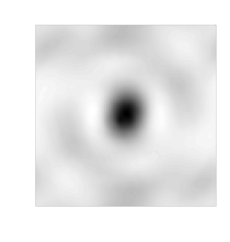
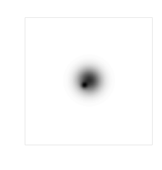
The ability of the algorithm to build a model of the true image using minimum DOF was tested by simulating an image composed of components using the same form of Asp as is used in the deconvolution process. It is clear that an image consisting of well separated Asp components will pass such a test (such a case will be equivalent to a test case for the normal CLEAN algorithm with only isolated unresolved sources). Therefore, a test image with an overlapping set of components at different scales (shown in the left panel of Fig. 1), was convolved with a typical interferometric PSF to form the dirty image (shown in the center panel of Fig. 1) and a noise image of type $\@vec{I^{N}}$ (RMS noise of $\approx 1$mJy) was added. This image was deconvolved to generate the model image shown in the right panel of Fig. 1. Only two Asp components were required to achieve convergence and the scale of these two components was automatically detected. In contrast, MS-Clean would need more components, unless of course the selected set of scales included precisly the two scales in the image. This demonstrates that under ideal conditions, where the true image is composed of only Asp shaped components, the algorithm does not introduce extra DOF. Although, in general where the true image is not strictly composed of only Asp shapes, it is impossible to design an algorithm which decomposes the image using minimum DOF, one can be optimistic that this algorithm will use fewer DOF compared to other algorithms. In practice, it is indeed observed that Asp-Clean uses about an order of magnitude fewer DOF than MS-Clean, which in turn uses few orders of magnitude fewer DOF than scale-less decomposition. Note that neither of these scale sensitive algorithms attempt to combine the components, e.g. construct a single component out of components located at the same pixel and of similar scales, to reduce the final number of components.

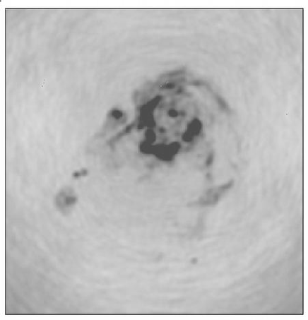
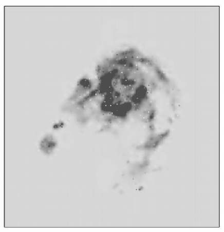
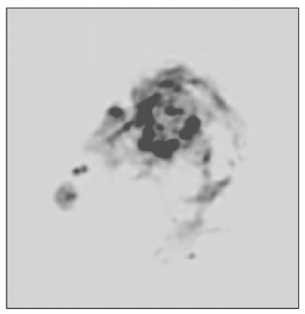
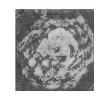
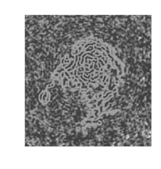
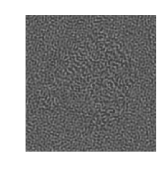
The top left panel of Fig. 2 shows the “M31” image used as the test image in our simulation. This was convolved with the PSF to generate the simulated dirty image shown in the top right panel. The resolution in the original image was $\approx 2^{\prime\prime}$ while the synthesized beam for the PSF was $\approx 2.5^{\prime\prime}$ in size. Asp deconvolution resulted in the Asp model image shown in the lower left panel of Fig. 2. The image is composed of a number of Aspen with the smallest being of the size of a single pixel (the bright “dots” in the image). Since the resolution element (the synthesized beam) is larger than the pixel size, this image needs to be smooth to the scale of the resolution element, which is shown in the lower right panel of Fig. 2. However, even without this smoothing operation, the Asp image is quite good showing all the morphological details of the original image. The emission, particularly the low level extended emission, is not broken up into small scales (as is in the case of scale-less deconvolution) and features with strong compact emission surrounded by extended emission are also properly reconstructed. The lower right panel shows the model image convolved with the estimated resolution element. Fig. 3 shows the residual images for the standard Cotton-Schwab Clean (CS-Clean), MS-Clean and the Asp-Clean algorithms. While the residuals for the CS-Clean and the MS-Clean are correlated with the large scale emission in the image, the Asp-Clean residuals are statistically consistent with the noise and have no significant correlated features at scales larger than the resolution element.

6 Acceleration methods

Figure 3: Figure shows the comparison of the residual images ($\@tens{B}\@vec{I^{M}}-\@vec{I^{d}}$) using the Cotton-Schwab Clean (left), MS-Clean (center) and Asp-Clean (right) algorithms. The Asp model image used to compute the Asp-Clean residual was the same as shown in Fig. 2. The residuals for Asp-Clean are consistent with the noise and contains no correlated features at scales larger than the resolution element. The residuals in the other two images are correlated with the large scale emission and are comparable in magnitude to the peak noise in the off-source regions. The Cotton-Schwab Clean was run for $50\,000$ components, MS-Clean for $20\,000$ components and Asp-Clean for $800$ components such that the peak residual was same for all cases. MS-Clean was run with 5 scales of sizes $0,3,5,10$ and 15 pixels.

For an $N$ Aspen set $\{P\}_{n}$ at iteration $n$, the dimensionality of the search space is $M\times N$ where $M$ is the number of parameters per Asp. The total number of parameters monotonically increases as a function of iteration number and step 4 becomes inefficient for complex images where the total number of Aspen can be several hundred.

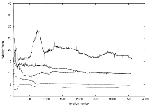
Figure 4 shows the evolution of the scale of the few largest Aspen for a typical test case image. To demonstrate the evolution of the scales, an Asp once introduced, was kept in the problem for all successive iterations. The top panel of Fig. 4 shows that after initial adjustment, the scale of most Aspen did not change significantly. The parts of the curves in the top panel with small derivatives correspond to small step-sizes in the minimization algorithm. Clearly, dropping Aspen which are unlikely to change significantly will greatly improve the performance with minimal adverse effect on the value of the objective function.

For a search space with constant curvature along all axis, the update step-size is proportional to the magnitude of the derivative along the various axis. Heuristically, the step-size for each Aspen in the minimization algorithm is proportional to the length of the derivative vector with respect to its parameters ($L_{k}=|\@vec{\nabla_{k}}\chi^{2}|$, where $\@vec{\nabla_{k}}$ corresponds to the derivative operator with respect to the parameters of the $k^{th}$ Asp only). This suggests a simple way of determining the active-set – i.e. by computing $L_{k}$ at the beginning of each minimization cycle and dropping Aspen for the current cycle for which $L_{k}$ is below a threshold $L_{o}$. Although this effectively assumes that the curvature along all axis is constant and is the same, and will result into some mistakes, one can recover from mistakes in later cycles since such a heuristic is applied at the beginning of each cycle. Assuming that the $\chi^{2}$ surface is well approximated by a parabola close to $\chi^{2}=0$, its slope progressively decreases as convergence is approached. $L_{o}$ therefore should also decrease as a function of convergence. The area under the residual image is indicative of the degree of convergence. Hence, a threshold of $L_{o}=\lambda\sum\@vec{I^{R}}$ was applied to $L_{k}$ at the beginning of each cycle to determine the active-set. The value of $\lambda$ controls the size of the active-set and needs to be determined empirically based on the available computing power and the complexity of the image - larger its value, the smaller the size of the active-set. Effects of the value of $\lambda$ on the rate of convergence and the quality of reconstruction has not yet been studied well. The lower panel of Fig. 4 shows the evolution of the scale of the same set of Aspen as shown in the top panel - but after applying this heuristic. Only the Aspen indicated by symbols on these curves, constitute the active set at each iteration. Roughly speaking, Aspen which were not evolving were automatically dropped from the problem. The figure also shows that the Aspen were dynamically included in the problem if it was estimated that adjusting them would have a significant impact on the $\chi^{2}$. Fig. 5 shows the number of Aspen along with the area under the residual image as a function of the iteration number. For the test image used, the initial iterations correspond to the larger Aspen. As the process progressed towards convergence, these large Aspen settled down, i.e. small adjustments to them had a lesser impact on convergence, than the addition of weaker and smaller scaled Aspen. Consequently, the initial Aspen dropped out of the problem, and at later times, convergence was achieved by keeping only a few (latest) Aspen. Effectively, this achieved a dynamic control on the dimensionality of the search space.

Figure 4: Evolution of a few large Aspen as a function of iterations for a test image. For the figure in the top panel, each Asp is kept in the problem after it is introduced. It shows that the size of most Aspen settle down and does not change significantly at each iteration. Flat portions in these curves imply insignificant step size in the optimization iterations. Dropping the Aspen in iterations where they do not change, significantly reduces computational cost with minimal adverse effect on convergence. The lower panel shows the evolution of the scales, after applying a heuristic at the beginning of each iteration to drop the Aspen which are unlikely to change significantly. At each iteration, only the Aspen marked with a symbol in this plot were retained for optimization for that iteration.

Figure 5: Figure showing the number of Aspen used along with the rate of convergence as a function of the iteration number. After initial rise in the number of Aspen, convergence was achieved by keeping only the latest few Aspen in the problem, effectively achieving a dynamic control on the dimensionality of the search space.

Strictly speaking, the active-set depends on the structure of the PSF and the inherent coupling of pixels in the image. Thresholding on the derivative vector and ignoring the curvature might result into dropping some axis with large curvature but small slope. Keeping them in the problem can potentially improve the rate of convergence. However that would require computation of the full covariance matrix, which is prohibitively expensive. An efficient algorithm to determine the structure of the covariance matrix, even approximately, will be most useful. Work for testing some of our ideas for such an algorithm is in progress.

7 Summary

Deconvolution of images with a large number of pixels with significant emission is inherently a high dimensional problem. The computational load depends on the structure of the covariance matrix, which in turn depends on the form of parameterization of the model image as well as on the structure of the PSF. It is possible to design efficient algorithms to decouple the PSF and the true image for images with a simple covariance structure (diagonal or band-diagonal matrix). The Pixon method is suitable for filled aperture telescopes since the PSF has a limited support making the covariance matrix strictly band diagonal at the worst, and the problem can be broken up into smaller local problems.

In addition to dealing with the inherent coupling of the pixels in the true image, interferometric imaging involves computing the coupling of the pixels due to the PSF, often through out the image. This has to be done for each trial model image (or its components) in search of the best model image. The Pixon method is therefore unsuitable for interferometric imaging. MS-Clean partly takes into account the inherent coupling of the pixels of the true image by representing it as a collection of components at a few scales. It ignores the coupling between these components but takes care of the coupling due to the PSF by pre-computing its effects. The advantage of this approach is that the computation of the coupling remains a scale-and-shift operation, which is efficient, while making the algorithm scale sensitive, albeit in a limited sense. The disadvantage is that it uses more DOF than necessary which leads to similar problems as in the CLEAN algorithm (that of breaking up of large scale emission). Non-symmetric structures are also difficult to accurately reconstruction.

Asp-Clean attempts to deal with these problems by explicitly solving the problem in the hyper-space of the Aspen parameters. The true image is modeled in the continuous space of Aspen. Since it is easy to parameterize the Aspen such that non-symmetric Aspen are also allowed, this algorithm deals with the problem of non-symmetric structures well, and results in a model image with the least DOF as compared to other algorithms for interferometric imaging. E.g., a purely elliptical gaussian shaped feature will be broken up into several symmetric components in the case of MS-Clean, while Asp-Clean can represent it with a single component. However the computation of the coupling is inefficient making the search for the parameters expensive. Since not all parameters continue to change throughout the search process, we have implemented heuristics to determine the active-set of parameters and dynamically limit the dimensionality of the search space. This improves the performance by an order of magnitude or more. However the overall runtime is still about a factor of three more than MS-Clean. Asp-Clean approach represents relaxation of compute-saving assumptions built into Clean and MS-Clean approaches. It is therefore inherently more compute intensive than other deconvolution algorithms. Although it is certainly useful to develop heuristics which will minimize redundant intermediate computations, the Asp decomposition is limited by the compute load for the search for the Asp parameters which in turn scales strongly with the size of the active-set at each iteration. Since the size of the active-set of Aspen is roughly a measure of the degree to which the non-orthogonality of the Aspen space (coupling between the Aspen) is incorporated in the algorithm, it is fair to expect it to impact the rate of convergence significantly. Faster convergence and possibly better reconstruction can be achieved with more computing power. Asp-Clean therefore scales better with the CPU speed, compared to other scale sensitive algorithms, and therefore has the potential of benefiting more from the Moore’s law of CPU speeds.

Currently we are using the standard routines for the search algorithm (conjugate gradient method and its variants or the Levenberg-Marquardt algorithm; see M. Galassi et al. (2002) for details). Fine tuning this minimization specifically for this problem will further improve the runtime performance. We use gaussians as the functional form for Asp. The scale of such Aspen is controlled by the full-width-at-half-maximum of the gaussian function. However there is no limit on the shape of the Aspen. More sophisticated functional forms which allow independent control on the shape as well the scale of the Asp will further reduce the number of components needed. Also, improving the heuristics to determine the active-set of Aspen, and making the heuristic computation itself efficient will be a worthwhile future direction of work.

Finally, we note that most of the Aspen with scale significantly larger than zero are found in the initial few hundred iterations, where the extra computational cost for Asp-Clean is well justified. The computational cost does not reduce for zero (or close to zero) scale Aspen. It may be most effective to develop heuristics to switch to other scale-less algorithms at late times which are more efficient for zero scale Aspen. Work in all these directions is in progress. Report on this on-going work and the impact of such algorithms on the imaging performance of future interferometric telescopes and imaging modes like mosaicking will be the subject matter of future papers.

The Asp-Clean algorithm as described in this paper is implemented as a Glish client in AIPS++ and can be run via a Glish script. Work is underway to incorporate this as one of the many available deconvolution algorithms in the standard AIPS++ interferometric imaging tool.