Monitoring water masers in star-forming regions

Abstract

An overview is given of the analysis of more than a decade of H₂O maser data from our monitoring program. We find the maser emission to generally depend on the luminosity of the YSO as well as on the geometry of the SFR. There appears to be a threshold luminosity of a few times 10${}^{4}~{}{\rm L}_{\odot}$ above and below which we find different maser characteristics.

guessConjecture

1 Introduction

Water masers in star-forming regions (SFRs) exhibit variability on short (days) and long (years) time scales. Therefore, while a single, one-time detection gives an important indication on the evolutionary status of the Young Stellar Object (YSO) with which the maser is associated, such an instantaneous picture does not teach us much more. We may hope to learn more by studying the behaviour of the maser emission with time. From the Arcetri H₂O maser catalogue (Comoretto et al. cat1; see also Brand et al. cat2, Valdettaro et al. cat3) we have selected about 50 H₂O masers in star-forming regions for monitoring. Because we want to investigate the dependence of the maser parameters on the energetic input of the driving source for star formation of all masses, a large range in far-infrared luminosity ($L_{\rm fir}$) of the YSO has been selected. As a first step in the systematic study of the maser variability, we have analyzed a sub-sample of 14 YSOs with luminosities between $20~{}{\rm L}_{\odot}$ and $1.8\times 10^{6}~{}{\rm L}_{\odot}$. The source names and various properties and derived parameters (see text) are listed in Table 1. A presentation of the available data for each of the 14 SFRs is given in Valdettaro et al. papI (2002).

Table 1: Observed and derived parameters of the H₂O maser sources analyzed in this paper

#	Source	$V_{\rm cl}^{\clubsuit}$	$d^{\dagger}$	$L_{\rm fir}^{\ddagger}$	$V_{\rm up}$a	$\Delta V_{\rm up}$a	$L_{\rm H_{2}O}^{up}$‡,b
		(km s-1)	(kpc)	(L⊙)	(km s-1)		(L⊙)
1	Sh 2-184	$-$30.8	2.2	7.9 (3)	$-$32.1	12.1	2.0 (–4)
2	L1455 IRS1	4.8	0.35	2.0 (1)	4.1	4.0	9.7 (–7)
3	NGC 2071	9.5	0.72	1.4 (3)	12.1	10.4	3.1 (–4)
4	Mon R2 IRS3	10.5	0.8	3.2 (4)	10.7	8.9	2.0 (–5)
5	Sh 2-269 IRS2	18.2	3.8	6.0 (4)	17.2	7.1	2.5 (–4)
6	W43 Main3	97.0	7.3	1.8 (6)	101.2	28.4	7.8 (–3)
7	G32.74$-$0.08	38.2	2.6	5.3 (3)	34.1	7.1	1.8 (–5)
8	G34.26+0.15	57.8	3.9	7.5 (5)	53.7	26.6	2.6 (–3)
9	G35.20$-$0.74	34.0	1.8	1.4 (4)	34.2	8.0	7.6 (–5)
10	G59.78+0.06	22.3	1.3	5.3 (3)	25.9	10.5	6.1 (–5)
11	Sh 2-128(H2O)	$-$71.0	6.5	8.9 (4)	$-$72.7	13.5	3.9 (–3)
12	NGC7129/FIRS2	$-$10.1	1.0	4.3 (2)	$-$4.6	12.5	6.9 (–5)
13	L1204-A	$-$7.1	0.9	2.6 (4)	$-$8.6	19.9	2.5 (–5)
14	L1204-G	$-$10.8	0.9	5.8 (2)	$-$18.1	14.5	2.3 (–5)
♣ Velocity of high-density gas (NH3,CS); for references see Valdettaro et al. papI (2002)
† For distance references, Valdettaro et al. papI (2002)
‡ Between brackets powers of 10
a $V_{\rm up}$ and $\Delta V_{\rm up}$ are the first and second moment of the upper envelope (see text)
b $L_{\rm H_{2}O}^{up}$ is the H2O luminosity derived from $\int F{\rm d}v$ over the upper envelope

2 Observations and data management

Although the monitoring campaign continues to the present day, the analysis presented here is based on observations carried out with the Medicina 32-m antenna (HPBW $\sim$ 1.^′9 at 22 GHz) between March 1987 and December 1999. Spectra were taken typically once every 2–3 months. The typical noise level in the spectra is 1.5 Jy; we estimate the calibration uncertainty to be $\sim 20$%. For the details of the observational parameters during the monitoring period we refer to Valdettaro et al. papI (2002) and references therein.

For each source we have obtained 35–50 spectra in the course of the campaign, thus there is a large amount of information on flux densities, velocities, and their variation with time, for all maser emission components. To be able to visually inspect the properties of the maser variation over time, and to enable a systematic analysis of the data, a compact way to display the data is of the essence. A very useful tool is the so-called $FVt$-diagram which shows flux density $F$ as a function of both velocity $V$ and time $t$, examples of which are shown in Fig. 1. This gives an overall description of the maser activity at a glance, and allows for a visual identification of maser bursts and possible velocity drifts.

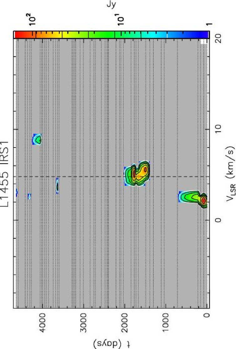
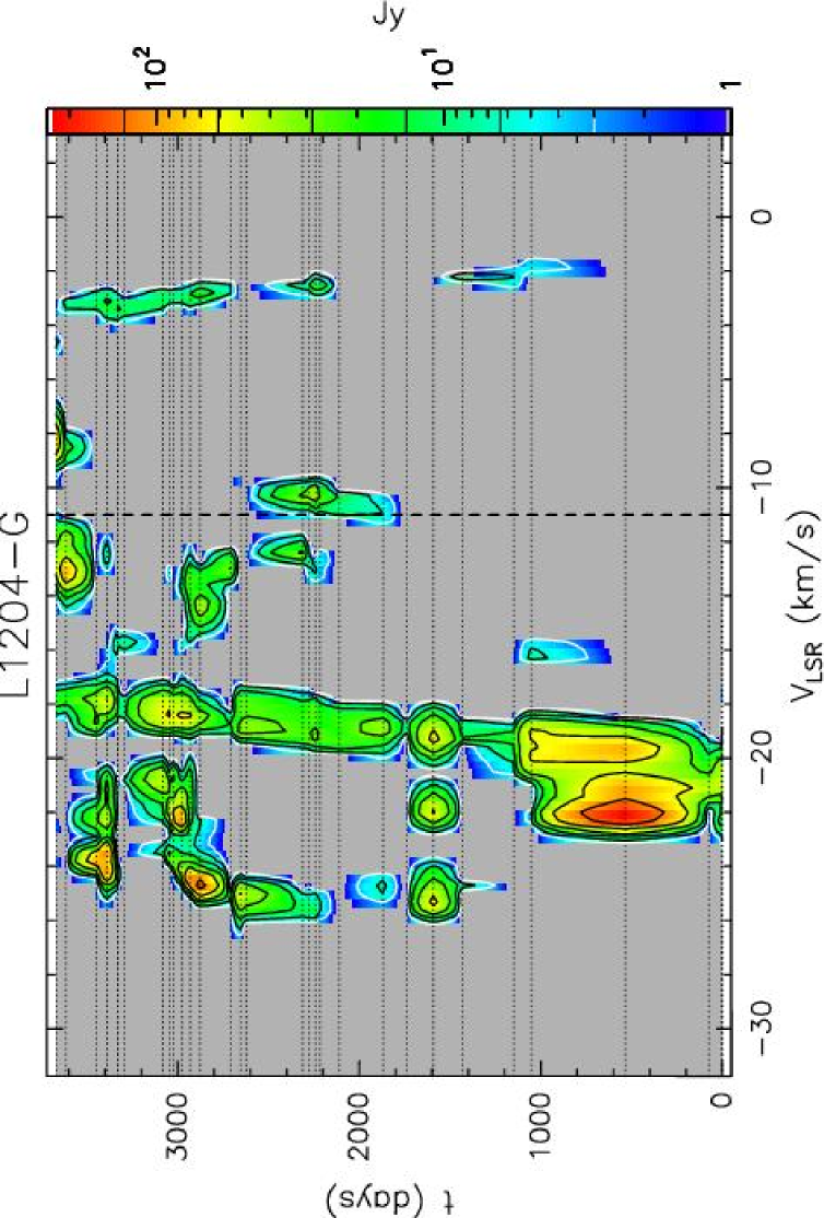
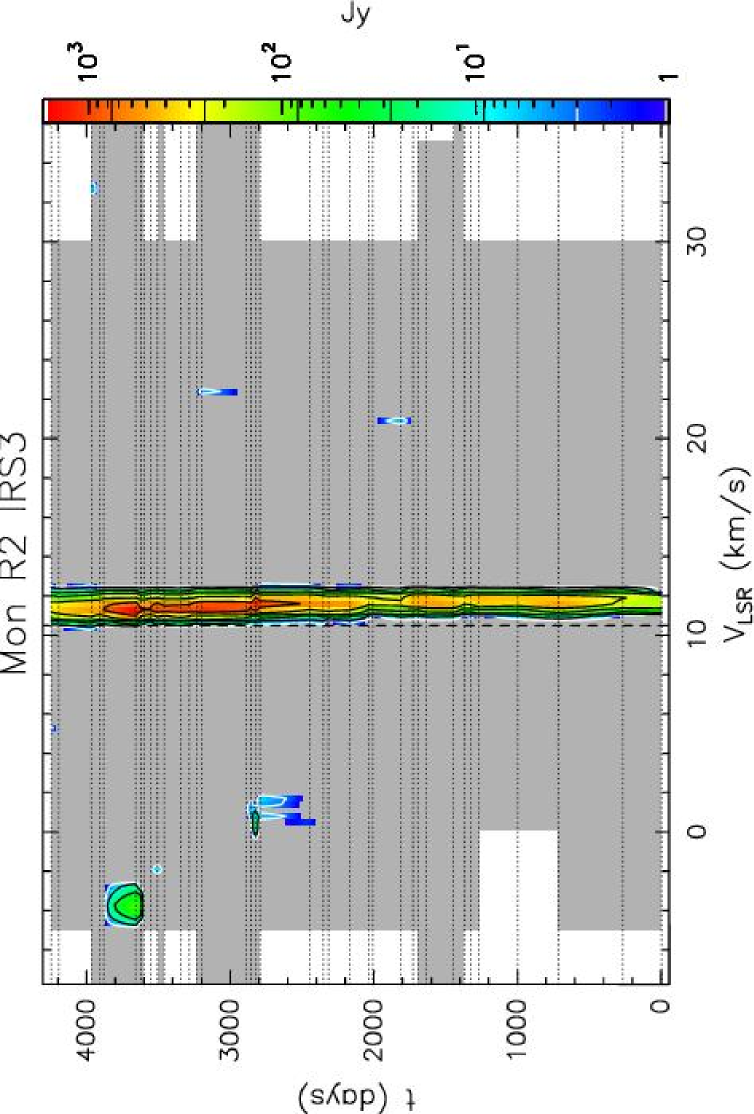
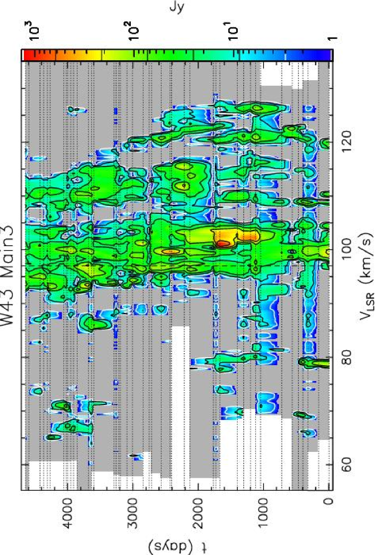
Figure 1: Examples of grey scale plot and contour map of the H₂O flux density versus velocity as a function of time ($FVt$-diagram). The vertical dashed line indicates the systemic velocity of the cloud, $V_{\rm cl}$. Horizontal dotted lines correspond to the dates of the observed spectra.

Other important tools in the analysis are the upper (lower) envelopes. These are hypothetical spectra, that show what the maser spectrum would look like if all velocity components were to emit at their maximum (minimum) level at the same time. These envelopes are created by assigning the maximum (minimum) signal detected (at 5$\sigma$-level) in each channel during the monitoring period. Integrating the upper envelope over all velocities leads to $L_{\rm H_{2}O}^{\rm up}$: the potential maximum maser luminosity the source could produce. This quantity is always higher than or equal to the observed maximum output $L_{\rm H_{2}O}^{\rm max}$, which is derived from the spectrum with the highest integrated flux density $S=\int FdV$. The frequency-of-occurrence or detection rate histogram indicates the percentage of time the flux density in each velocity-channel exceeded the 5$\sigma$-level (see Fig. 4b). And finally, it is convenient to characterize the mean maser velocity and its dispersion by computing $V_{\rm up}$ and $\Delta V_{\rm up}$: the first, respectively second moment of the upper envelope. Similarly, $V_{\rm fr}$ and $\Delta V_{\rm fr}$ are defined from the detection rate histograms.

3 Analysis

During the course of the data analysis a simple empirical picture has emerged for maser emission around a YSO, that takes into account all findings. A basic assumption in this framework is that around a YSO there are many potential maser sites that can be excited by shocks caused by impact with an outflow-jet originating at the YSO if the appropriate masing conditions can be created. This will be seen to not only depend on the $L_{\rm fir}$ of the YSO, but also on the directional properties of the jet. Because it is likely that within the Medicina beam there will be more than one YSO (as there will be within one IRAS beam), we are really investigating global properties of a cluster, rather than of a single object. In this context $L_{\rm fir}$ can be seen as an upper limit to the luminosity of the brightest YSO and in this sense allows discrimination between the environments of YSOs of different luminosities. Furthermore we note that while there is an established correlation between the energetics of large-scale outflows (as measured e.g. in CO) and of water masers, it is also true that the velocity extent of the bulk of the outflowing gas is typically less than 10 km s^-1, while maser emission can occur over a range of velocities of 100 km s^-1 or more. This means that maser components, certainly those at large red- or blue-shifted velocities (with respect to that of the parent cloud) must be directly excited by high-velocity gas originating from the YSO. This jet-component also entrains the ambient gas, which forms the (slower-moving) large-scale outflow.

Due to space limitations only some of the results can be presented here; for a complete account, subtleties, and caveats see Brand et al. papII (2003).

1. From the fact that $V_{\rm up}\approx V_{\rm fr}$, we see that the velocity at which the maser emission is most intense is also that where it occurs most often. The representative mean maser velocity, $V_{\rm up}$, is always within 7.5 km s^-1 of the parent molecular cloud: $V_{\rm up}-V_{\rm cl}=-0.4\pm 3.5$ km s^-1. This implies that maser emission is maximum for zero projected velocities with respect to the local environment, i.e. when the plane of the shock that creates the masing conditions is along the line-of-sight (cf. Elitzur et al. elitzur).

2. $L_{\rm H_{2}O}^{\rm up}$ correlates well with the luminosity of the YSO; a power-law fit gives $L_{\rm H_{2}O}^{\rm up}$= $6.4\times 10^{-8}$$L_{\rm fir}$^0.81±0.07. This is in good agreement with the slope of 1.00$\pm$0.07 of a fit to the outer envelope of the distribution of single observations of many maser sources obtained by Wouterloot et al. paper6 (1995).

3. As can be seen from the FVt-diagrams in Fig. 1, maser variability is a complex affair. Nevertheless, its overall behaviour is described by the ratio $S_{\rm max}/S_{\rm mean}$ between the maximum and the mean integrated flux densities over the whole monitoring period. From Fig. 2a one sees that high-luminosity YSOs tend to be associated with more stable masers. This can be understood in the context of the basic framework assumption mentioned above: around lower-luminosity YSOs a smaller number of maser components gets excited, and their intrinsic time-variability will dominate the total output; near higher-luminosity YSOs a larger number of components may be simultaneously excited, reducing the effect of their individual time-variability.

Figure 2: A selection of the results. The numbers inside the data-circles correspond to the object-numbers in Table 1. a. The ratio of maximum and mean integrated flux density as a function of the luminosity of the YSO. b. The total velocity extent of the maser emission (from the frequency-of-occurrence histograms) as a function of the maser luminosity $L_{\rm H_{2}O}^{\rm up}$. c. The number of velocity components in the spectrum with the highest integrated flux density during monitoring, as a function of $L_{\rm H_{2}O}^{\rm max}$, the maser luminosity determined from that same spectrum. d. As c, but as a function of the velocity range of the emission in the spectrum.

4. $\Delta V_{\rm tot}$ is the total velocity extent of the maser emission in the frequency-of-occurrence histograms; it is shown as a function of $L_{\rm H_{2}O}^{\rm up}$ in Fig. 2b. The data show that a more luminous YSOs can excite maser emission over a larger velocity range, but does not necessarily always do so, as this also depends on the local environment: the alignment of the jets with respect to the line-of-sight, and the local gas density will play a role too (see also items 9 & 10).

5. To excite all the potential sites of maser emission, sufficient energy is required to pump them. This energy is delivered by shocks, created by jets driven by the YSO. To excite maser emission at large (with respect to the parent cloud) velocity, powerful flows are needed, and hence more luminous YSOs. These will thus be associated with maser spectra containing more emission components over a larger range in velocity, as is indeed found: Fig. 2c, d.

6. The $FVt$-diagrams can be used to study bursts of maser emission or to determine velocity drifts of individual maser components. Regarding the former, the limiting factor is our relatively large sampling interval of 60$-$100 days, while identifying individual velocity components and following them in time is only possible for masers with few components (cf. Mon R2 or L1204-G in Fig. 1), or for components at velocities far from the crowded parts of the spectrum. From an analysis of 15 suitable maser components we found velocity gradients (both positive and negative) ranging between 0.02 and 1.8 km s^-1yr^-1. From an analysis of 14 bursts in 9 components in 6 sources we found durations $\Delta t\sim 63-900$ days; the lower value is determined by our sampling interval, the higher value by the fact that bursts of longer duration are not recognized as such. Flux density increases $\Delta F$ ranged from a few tens to a few thousand percent. Both $\Delta t$ and $\Delta F$ were found to decrease with increasing velocity offset of the maser component; this is consistent with what is indicated by the shape of the upper envelopes and the detection rate histograms.

Figure 3: The integrated flux density, normalized by that of the upper envelope, as a function of time. The panels illustrate the ’super-variability’ present in the maser output of the three sources shown.

7. In addition to occasional outbursts of individual maser components, in several sources a long-term, possibly periodic variability is detected in the total maser output. Fig. 3 shows this for three of the best cases. The estimated duration of a full cycle varies between 5.5 (Sh 2 184, Sh 2 269) and 11 (Sh 2 128) years. This ’super-variability’ might be caused by periodic variation in the YSO-power supply (which drives the jet that creates the shocks that excite the maser).

8. In Fig. 4a we show the scaled velocity-time-intensity diagrams, with $L_{\rm fir}$ increasing from bottom to top, and from left to right. Note how for $L_{\rm fir}$$\geq 3\times 10^{4}$ L_⊙ the emission becomes increasingly complex: from Mon R2 IRS3 to W43 Main3 the maser emission changes from being dominated by a single component to being highly structured and multi-component; the velocity extent of the emission also increases. For lower $L_{\rm fir}$ there is a variety of morphologies, but without a systematic trend with $L_{\rm fir}$, and with a smaller velocity range. The source with the lowest $L_{\rm fir}$ in the sample ($\sim 20$ L_⊙) has not been detected most of the time.

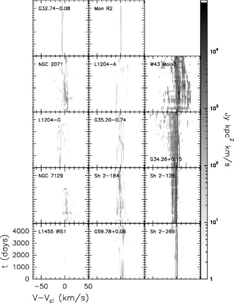
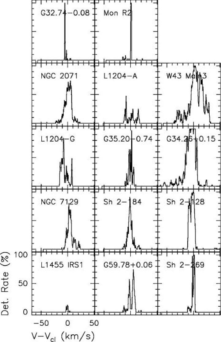
Figure 4: a. Left: $FVt$-maps, like the ones shown in Fig 1, but the flux densities are scaled by $d^{2}$ and the logarithmic intensity scale is the same for all panels, thus as if the sources were at the same distance. The velocities are relative to the parent-cloud velocity $V_{\rm cl}$. The sources are ordered in $L_{\rm fir}$ of the YSO, which increases from bottom to top and from left to right. b. Right: Detection rate histograms. Ordered in $L_{\rm fir}$ as in a.

9. Fig. 4b shows the scaled frequency-of-occurrence diagrams, ordered in $L_{\rm fir}$ as in the FVt-diagrams. We see that for YSOs with $L_{\rm fir}$$\geq 3\times 10^{4}$ L_⊙ there is at least one velocity component of the H₂O maser with a detection rate of 100%, and it is always very close to $V_{\rm cl}$. This is in agreement with what was found by Wouterloot et al. paper6 (1995) using a very different sample and observational approach. For sources with lower $L_{\rm fir}$ the typical maser detection rate (above the 5$\sigma$-level) is 75–80%. The YSO with the lowest $L_{\rm fir}$ has a detection rate of only $\sim 10$%. The steep decline of the histograms with velocity away from $V_{\rm cl}$ indicates that more blue- and red-shifted maser components have shorter lifetimes than those near the systemic velocity. An interesting feature of the histograms is the ’tail’, consisting of a collection of smaller peaks, which for sources with $L_{\rm fir}$$\geq 3\times 10^{4}$ L_⊙ is preferentially on the blue side of the main peak (except only for Sh 2 128). As mentioned earlier, maser amplification is maximum in the plane of the shocks, where the gain path is longest (Elitzur et al. elitzur). For high-velocity blue- and red-shifted components the plane of the shock is perpendicular to the line-of-sight, and the gain path is short. But if a well-collimated jet is precisely aligned with the line-of-sight, the maser can amplify the background continuum (from the Hii region) and the blue-shifted components can become more intense. The strength and velocity offset of the maser feature will be determined by the jet’s collimation, its alignment with the line-of-sight, and by the background radio continuum (hence by the luminosity of the YSO). Fig. 4b shows that in our sample these effects combine most favourably in G34.26$-$0.15 and W43 Main3. High-velocity red-shifted components will always be weaker, because they cannot amplify the continuum background. If there is no outflow, or if it is driven by a lower-luminosity YSO, high-velocity components will not be seen at all. If the maser emission comes primarily from a protostellar disk, blue- and red-shifted components can be seen, but at velocities close to $V_{\rm cl}$. Thus, maser emission would also be a function of the geometry of the SFR, in particular of the orientation of the beam of the outflow with respect to the line-of-sight to the YSO.

10. It appears that sources with $4\times 10^{2}$ L${}_{\odot}\leq$ $L_{\rm fir}$$\leq 6\times 10^{4}$ L_⊙ (from NGC7129 to Sh 2 269 in order of increasing luminosity) have similar (scaled) upper envelopes (not shown), with peak values of $log[F_{\nu}d^{2}]\sim 3$ and with comparable velocity range. Outside this homogeneous group of sources we find on the one hand the lowest-luminosity source ($L_{\rm fir}$$\approx 20$ L_⊙) with $log[F_{\nu}d^{2}]$ two orders of magnitude smaller and with a narrower velocity range of the emission, and on the other hand the sources with higher luminosity ($L_{\rm fir}$$\geq 6\times 10^{4}$ L_⊙), with peak values of $log[F_{\nu}d^{2}]\sim 4-5$ and a larger extent in velocity. These distinctions may reflect three different regimes of maser excitation: In the lowest luminosity sources, the maser excitation occurs on a small ($\sim 100$ AU) spatial scale and might be produced by the stellar jets visible in the radio continuum. The outflows are either less powerful or impact with a lower-density ambient medium, where conditions are not suitable to create masers. In the intermediate luminosity class, the larger energetic input from the jet, as well as the presence of a higher-density molecular gas, are the main agents that determine the conditions for maser excitation. In the most luminous sources, conditions for maser excitation are similar to those in the previous category, but in this case the energetic input is so large that all potential maser sites are excited, and the determining factor is the YSO luminosity.

4 Summary

We have presented an analysis of more than 10 years-worth of water maser data of 14 SFRs. There is a clear overall dependence of the parameters of the maser emission on the YSO luminosity. In addition, we find the existence of different $L_{\rm fir}$ regimes and a threshold YSO-luminosity (of $\sim 10^{4}$ L_⊙) that can account for the various observed characteristics of the H₂O maser emission. Furthermore, the maser emission is found to depend on the morphology of the SFR, particularly the orientation of the outflow-jet with respect to the line-of-sight, and the density of the parent molecular environment. For the full detailed analysis, see Brand et al. papII (2003).

References

- (1) Brand J., Cesaroni R., Caselli P., et al.: 1994, A&AS 103, 541
- (2) Brand J., Cesaroni R., Comoretto G., et al.: 2003, A&A 407, 573
- (3) Comoretto G., Palagi F., Cesaroni R., et al.: 1990, A&AS 84, 179
- (4) Elitzur M., Hollenbach D.J., and McKee C.F.: 1989, ApJ 346, 983
- (5) Valdettaro R., Palla F., Brand J., et al.: 2001, A&A 368, 845
- (6) Valdettaro R., Palla F., Brand J., et al.: 2002, A&A 383, 266
- (7) Wouterloot J.G.A., Fiegle K., Brand J., and Winnewisser G.: 1995, A&A 301, 236 (Erratum: 1997, A&A 319, 360)