Microlensing towards LMC and M31

Abstract

The nature and the location of the lenses discovered in the microlensing surveys done so far towards the LMC remain unclear. Motivated by these questions we computed the optical depth for the different intervening populations and the number of expected events for self-lensing, using a recently drawn coherent picture of the geometrical structure and dynamics of the LMC. By comparing the theoretical quantities with the values of the observed events it is possible to put some constraints on the location and the nature of the MACHOs. Clearly, given the large uncertainties and the few events at disposal it is not yet possible to draw sharp conclusions, nevertheless we find that up to 3-4 MACHO events might be due to lenses in LMC, which are most probably low mass stars, but that hardly all events can be due to self-lensing. The most plausible solution is that the events observed so far are due to lenses belonging to different intervening populations: low mass stars in the LMC, in the thick disk, in the spheroid and some true MACHOs in the halo of the Milky Way and the LMC itself. We report also on recent results of the SLOTT-AGAPE and POINT-AGAPE collaborations on a search for microlensing events in direction of the Andromeda galaxy, by using the pixel method. The detection of 4 microlensing events, some likely to be due to self–lensing, is discussed. One microlensing light curve is shown to be compatible with a binary lens. The present analysis still does not allow us to draw conclusions on the MACHO content of the M31 galaxy.

1 Introduction

Since Paczyński’s original proposal[1] gravitational microlensing has been proben to be a powerful tool for the detection of the dark matter component in galactic haloes in the form of MACHOs. Searches in our Galaxy towards LMC[2, 3] show that up to 20% of the halo could be formed by objects of around $M\sim 0.4\,M_{\odot}$.

However, the location and the nature of the microlensing events found so far towards the Large Magellanic Cloud (LMC) is still a matter of controversy. The MACHO collaboration found 13 to 17 events in 5.7 years of observations, with a mass for the lenses estimated to be in the range $0.15-0.9~{}M_{\odot}$ assuming a standard spherical Galactic halo[2] and derived an optical depth of $\tau=1.2^{+0.4}_{-0.3}\times 10^{-7}$. The EROS2 collaboration[4] announced the discovery of 4 events based on three years of observation but monitoring about twice as much stars as the MACHO collaboration. The MACHO collaboration monitored primarily 15 deg² in the central part of the LMC, whereas the EROS2 experiment covers a larger solid angle of 64 deg² but in less crowded fields. The EROS2 microlensing rate should thus be less affected by self-lensing. This might be the reason for the fewer events seen by EROS2 as compared to the MACHO experiment.

The hypothesis for a self-lensing component was discussed by several authors [5, 6, 7, 8]. The analysis of Jetzer et al. [9] and Mancini et al. [10] has shown that probably the observed events are distributed among different galactic components (disk, spheroid, galactic halo, LMC halo and self-lensing). This means that the lenses do not belong all to the same population and their astrophysical features can differ deeply one another.

Some of the events found by the MACHO team are most probably due to self-lensing: the event MACHO-LMC-9 is a double lens with caustic crossing[11] and its proper motion is very low, thus favouring an interpretation as a double lens within the LMC. The source star for the event MACHO-LMC-14 is double[12] and this has allowed to conclude that the lens is most probably in the LMC. The expected LMC self-lensing optical depth due to these two events has been estimated to lie within the range[12] $1.1-1.8\times 10^{-8}$, which is still below the expected optical depth for self-lensing even when considering models giving low values for the optical depth. The event LMC-5 is due to a disk lens[13] and indeed the lens has even been observed with the HST. The other stars which have been microlensed were also observed but no lens could be detected, thus implying that the lens cannot be a disk star but has to be either a true halo object or a faint star or brown dwarf in the LMC itself.

Thus up to now the question of the location of the observed MACHO events is unsolved and still subject to discussion. Clearly, with much more events at disposal one might solve this problem by looking for instance at their spatial distribution. To this end a correct knowledge of the structure and dynamics of the luminous part of the LMC is essential, and we take advantage of the new picture drawn by van der Marel et al. [14, 15, 16].

Searches towards M31, nearby and similar to our Galaxy, have also been proposed[17, 18, 19]. This allows to probe a different line of sight in our Galaxy, to globally test M31 halo and, furthermore, the high inclination of the M31 disk is expected to provide a strong signature (spatial distribution) for halo microlensing signals.

Along a different direction, results of a microlensing survey towards M87, where one can probe both the M87 and the Virgo cluster haloes, have also been presented[20].

For extragalactic targets, due to the distance, the sources for microlensing signals are not resolved. This claims for an original technique, the pixel method, the detection of flux variations of unresolved sources[21, 22, 23], the main point being that one follows flux variations of every pixel in the image instead of single stars.

We discuss here the results from two different survey of M31 aimed at the detection of microlensing events, carried out by the SLOTT-AGAPE[24, 25] and by the POINT-AGAPE collaborations[26, 27]. The WeCapp[28, 29] and the MEGA[30] collaborations have also presented a handful of microlensing events.

2 LMC model

In a series of three interesting papers [14, 15, 16], a new coherent picture of the geometrical structure and dynamics of LMC has been given. In the following we adopt this model and use the same coordinate systems and notations as in van der Marel. We consider an elliptical isothermal flared disk tipped by an angle $i=34.7^{\circ}\pm 6.2^{\circ}$ as to the sky plane, with the closest part in the north-east side. The center of the disk coincides with the center of the bar and its distance from us is $D_{0}=50.1\pm 2.5\,\mathrm{kpc}$. We take a bar mass $M_{\mathrm{bar}}=1/5\,M_{\mathrm{disk}}$ with $M_{\mathrm{bar}}+M_{\mathrm{disk}}=M_{\mathrm{vis}}=2.7\times 10^{9}\,\mathrm{M}_{\odot}$.

The vertical distribution of stars in an isothermal disk is described by the $\mathrm{sech}^{2}$ function; therefore the spatial density of the disk is modeled by:

$$\rho_{\mathrm{d}}=\frac{N\,M_{\mathrm{d}}}{4\pi\,q\,R_{\mathrm{d}}^{2}\,\zeta_{\mathrm{d}}(0)}\;\mathrm{sech}^{2}\left(\frac{\zeta}{\zeta_{\mathrm{d}}(R)}\right)e^{-{\frac{1}{R_{\mathrm{d}}}}\sqrt{\left(\frac{\xi}{q}\right)^{2}+{\eta}^{2}}}~{},$$ (1)

where $q=0.688$ is the ellipticity factor, $R_{\mathrm{d}}=1.54\,\mathrm{kpc}$ is the scale length of the exponential disk, $R$ is the radial distance from the center on the disk plane. ${\zeta_{\mathrm{d}}(R)}$ is the flaring scale height, which rises from 0.27 kpc to 1.5 kpc at a distance of 5.5 kpc from the center[16], and is given by

$${\zeta_{\mathrm{d}}(R)}=0.27+1.40\,\tanh\left(\frac{R}{4}\right)~{}.$$

$N=0.2765$ is a normalization factor that takes into account the flaring scale height.

In a first approach[9] we have described the bar by a Gaussian density profile following Gyuk et al. [31], whereas in a following paper[10] we choose, instead, a bar spatial density that takes into account its boxy shape[8]:

$$\rho_{\mathrm{b}}=\frac{2\,M_{\mathrm{b}}}{\pi^{2}\,R_{\mathrm{b}}^{2}\,\,\Xi_{\mathrm{b}}}\,e^{-\left(\frac{\Xi}{\,\Xi_{\mathrm{b}}}\right)^{2}}\,e^{-\,\frac{1}{R_{\mathrm{b}}^{4}}\left(\Upsilon^{2}+\,\zeta^{2}\right)^{2}},$$ (2)

where $\Xi_{\mathrm{b}}=1.2\,\mathrm{kpc}$ is the scale length of the bar axis, $R_{\mathrm{b}}=0.44\,\mathrm{kpc}$ is the scale height along a circular section (for a more detailed discussion and definition of the coordinate system see [10]).

The column density, projected on the $x-y$ sky plane is plotted in Fig. 1, giving a global view of the LMC shape for a terrestrial observer, together with the positions of the microlensing events detected by the MACHO (filled stars and empty diamonds) and EROS (filled triangles) collaborations, and the direction of the line of nodes. The maximum value of the column density, $41.5\times 10^{7}~{}\mathrm{M}_{\odot}\,\mathrm{kpc}^{-2}$, is assumed in the center of LMC.

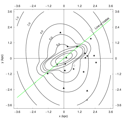
Figure 1: Projection on the sky plane ($x-y$ plane) of the column density of the LMC disk and bar. The numerical values on the contours are in $10^{7}\mathrm{M}_{\odot}\mathrm{kpc}^{-2}$ units. The three innermost contours correspond to $10$, $20$ and $30\times 10^{7}\mathrm{M}_{\odot}\mathrm{kpc}^{-2}$. The locations of the MACHO (black stars and empty diamonds) and EROS (triangles) microlensing candidates are also shown.

We use two different models to describe the halo profile density: a spherical halo and an ellipsoidal halo. The values of the parameters have been chosen so that the models have roughly the same mass within the same radius. In the spherical model we neglect the tidal effects due to our Galaxy, and we adopt a classical pseudo-isothermal spherical density profile:

$$\rho_{\mathrm{h,S}}=\rho_{\mathrm{0,S}}\left(1+\frac{R^{2}}{a^{2}}\right)^{-1}\theta(R_{\mathrm{t}}-R),$$ (3)

where $a$ is the LMC halo core radius, $\rho_{0,\mathrm{S}}$ the central density, $R_{\mathrm{t}}$ a cutoff radius and $\theta$ the Heaviside step function. We use $a=2$ kpc. We fix the value for the mass of the halo within a radius of 8.9 kpc equal to[16] $5.5\times 10^{9}~{}\mathrm{M}_{\odot}$ that implies $\rho_{0,\mathrm{S}}$ equal to $1.76\times 10^{7}\,~{}\mathrm{M}_{\odot}\,\mathrm{kpc}^{-3}$. Assuming a halo truncation radius[16], $R_{\mathrm{t}}=15$ kpc, the total mass of the halo is $\approx 1.08\times 10^{10}\,~{}\mathrm{M}_{\odot}$.

For the galactic halo we assume a spherical model with density profile given by:

$$\rho_{\mathrm{GH}}=\rho_{\mathrm{0}}\frac{R_{\mathrm{C}}^{2}+R_{\mathrm{S}}^{2}}{R_{\mathrm{C}}^{2}+R^{2}},$$ (4)

where $R$ is the distance from the galactic center, $R_{\mathrm{C}}=5.6\,\,\mathrm{kpc}$ is the core radius, $R_{\mathrm{S}}=8.5\,\,\mathrm{kpc}$ is the distance of the Sun from the galactic center and $\rho_{\mathrm{0}}=7.9\times 10^{6}\,~{}\mathrm{M}_{\odot}\,\mathrm{kpc}^{-3}$ is the mass density in the solar neighbourhood.

3 LMC optical depth

The computation is made by weighting the optical depth with respect to the distribution of the source stars along the line of sight (see Eq.(7) in Jetzer et al. [9]):

$$\tau={\frac{4\pi G}{c^{2}}}{\frac{\int_{0}^{\infty}\left[\int_{0}^{D_{\mathrm{os}}}{\frac{D_{\mathrm{ol}}(D_{\mathrm{os}}-D_{\mathrm{ol}})}{D_{\mathrm{os}}}}\rho_{\mathrm{l}}\,dD_{\mathrm{ol}}\right]\rho_{\mathrm{s}}\,dD_{\mathrm{os}}}{\int_{0}^{\infty}\rho_{\mathrm{s}}\,dD_{\mathrm{os}}}}\;.$$ (5)

$\rho_{\mathrm{l}}$ denotes the mass density of the lenses, $\rho_{\mathrm{s}}$ the mass density of the sources, $D_{\mathrm{ol}}$ and $D_{\mathrm{os}}$, respectively, the distance observer-lens and observer-source.

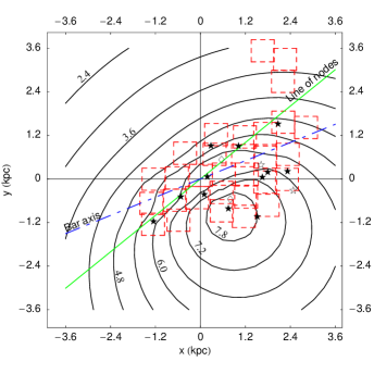
Figure 2: Spherical halo model: contour map of the optical depth for lenses in the LMC halo. The locations of the MACHO fields and of the microlensing candidates are also shown. The numerical values are in $10^{-8}$ units.

In Fig. 2 we report the optical depth contour maps for lenses belonging to the halo of LMC in the case of spherical model in the hypothesis that all the LMC dark halo consists of compact lenses. The ellipsoidal model leads to similar results[10]. A striking feature of the map is the strong near-far asymmetry.

For the spherical model, the maximum value of the optical depth, $\tau_{\mathrm{max,S}}\simeq 8.05\times 10^{-8}$, is assumed in a point falling in the field number 13, belonging to the fourth quadrant, at a distance of $\simeq 1.27$ kpc from the center. The value in the point symmetrical with respect to the center, belonging to the second quadrant and falling about at the upward left corner of the field 82, is $\tau_{\mathrm{S}}\simeq 4.30\times 10^{-8}$. The increment of the optical depth is of the order of $\approx 87\%$, moving from the nearer to the farther fields.

In Fig. 3 we report the optical depth contour map for self-lensing, i. e. for events where both the sources and the lenses belong to the disk and/or to the bulge of LMC. As expected, there is almost no near-far asymmetry and the maximum value of the optical depth, $\tau_{\mathrm{max}}\simeq 4.80\times 10^{-8}$, is reached in the center of LMC. The optical depth then rapidly decreases, when moving, for instance, along a line going through the center and perpendicular to the minor axis of the elliptical disk, that coincides also with the major axis of the bar. In a range of about only $0.80\,\mathrm{kpc}$ the optical depth quickly falls to $\tau\simeq 2\times 10^{-8}$, and afterwards it decreases slowly to lower values.

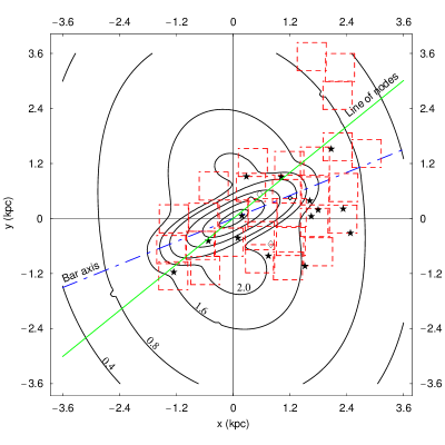
Figure 3: Contour map of the optical depth for self-lensing. The locations of the MACHO fields and of the microlensing candidates are also shown. The numerical values are in $10^{-8}$ units. The innermost contours correspond to values $2.4\times 10^{-8}$, $3.2\times 10^{-8}$, $4.0\times 10^{-8}$ and $4.6\times 10^{-8}$ respectively.

4 LMC self-lensing event rate

An important quantity, useful for the physical interpretation of microlensing events, is the distribution $\frac{\mathrm{d}\Gamma}{\mathrm{d}\,T_{\mathrm{E}}}$, the differential rate of microlensing events with respect to the Einstein time $T_{\mathrm{E}}$. In particular it allows us to estimate the expected typical duration and their expected number. We evaluated the microlensing rate in the self-lensing configuration, i. e. lenses and sources both in the disk and/or in the bar of LMC. We have taken into account the transverse motion of the Sun and of the source stars. We assumed that, to an observer comoving with the LMC center, the velocity distribution of the source stars and lenses have a Maxwellian profile, with spherical symmetry.

In the picture of van der Marel et al. within a distance of about 3 kpc from the center of LMC, the velocity dispersion (evaluated for carbon stars) along the line of sight can be considered constant, $\sigma_{\mathrm{los}}=20.2\pm.5$ km/s. Most of the fields of the MACHO collaboration fall within this radius and, furthermore, self-lensing events are in any case expected to happen in this inner part of LMC. Therefore, we adopted this value, even if we are aware that the velocity dispersion of different stellar populations in the LMC varies in a wide range, according to the age of the stellar population: $\simeq 6$ km/s for the youngest population, until $\simeq 30$ km/s for the older ones[31].

We need now to specify the form of the number density. Assuming that the mass distribution of the lenses is independent of their position[32] in LMC (factorization hypothesis), the lens number density per unit mass is given by

$${\frac{\mathrm{d}n_{\mathrm{l}}}{\mathrm{d}\mu}}={\frac{\rho_{\mathrm{d}}+\rho_{\mathrm{b}}}{\mathrm{M}_{\odot}}}\,{\frac{\mathrm{d}n_{0}}{\mathrm{d}\mu}},$$ (6)

where we use ${\frac{\mathrm{d}n_{0}}{\mathrm{d}\mu}}$ as given in Chabrier[33] ($\mu=M/M_{\odot}$). We consider both the power law and the exponential initial mass functions. However, we find that our results do not depend strongly on that choice and hereafter, we will discuss the results we obtain by using the exponential IMF only.

Let us note that, considering the experimental conditions for the observations of the MACHO team, we use as range for the lens masses $0.08\leq\mu\leq 1.5$. The lower limit is fixed by the fact that the lens must be a star in LMC, while the upper limit is fixed by the requirement that the lenses are not resolved stars.

We compute the “field exposure”, $E_{\mathrm{field}}$, defined, as in Alcock et al. [2], as the product of the number of distinct light curves per field by the relevant time span, paying attention to eliminate the field overlaps; moreover we calculate the distribution ${\frac{\mathrm{d}\Gamma}{\mathrm{d}T_{\mathrm{E}}}}$ along the line of sight pointing towards the center of each field. In this way we obtain the number of expected events for self-lensing, field by field, given by

$$N_{\mathrm{SL,field}}=E_{\mathrm{field}}\int_{0}^{\infty}\,{\frac{\mathrm{d}\Gamma}{\mathrm{d}T_{\mathrm{E}}}}\,E(T_{\mathrm{E}})\,\mathrm{d}\,T_{\mathrm{E}}\;,$$ (7)

where $E(T_{\mathrm{E}})$ is the detection efficiency.

Summing over all fields we find that the expected total number of self-lensing events is $\sim 1.2$, while we would get $\sim 1.3$ with the the double power law IMF; in both cases altogether 1-2 events[10]. Clearly, taking also into account the uncertainties in the parameter used following the van der Marel model for the LMC the actual number could also be somewhat higher but hardly more than our upper limit estimate of about 3-4 events given in[9].

4.1 Self-lensing events discrimination

It turns out that, in the framework of the LMC geometrical structure and dynamics outlined above, a suitable statistical analysis allows us to exclude from the self-lensing population a large subset of the detected events. To this purpose, assuming all the 14 events as self-lensing, we study the scatter plots correlating the self-lensing expected values of some meaningful microlensing variables with the measured Einstein time or with the self-lensing optical depth. In this way we can show that a large subset of events is clearly incompatible with the self-lensing hypothesis.

We have calculated the self-lensing distributions $\left({\frac{\mathrm{d}\Gamma}{\mathrm{d}T_{\mathrm{E}}}}\right)_{\varepsilon}$ of the rate of microlensing events with respect to the Einstein time $T_{\mathrm{E}}$, along the lines of sight towards the 14 events found by the MACHO collaboration, in the case of a Chabrier exponential type IMF. With these distributions we have calculated the modal $T_{\mathrm{E,mod}}$, the median $T_{\mathrm{E},\,50\,\%}$ and the average $<T_{\mathrm{E}}>$ values of the Einstein time.

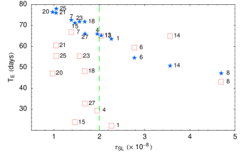
Figure 4: Scatter plot of the observed (empty boxes) values of the Einstein time and of the expected values of the median $T_{\mathrm{E},50\,\%}$ (filled stars), with respect to the self-lensing optical depth evaluated along the directions of the events.

In Fig. 4 we report on the $y$–axis the observed values of $T_{\mathrm{E}}$ (empty boxes) as well as the expected values for self-lensing of the median $T_{\mathrm{E}\,,50\,\%}$ (filled stars) evaluated along the directions of the events. On the $x$–axis we report the value of the self-lensing optical depth calculated towards the event position; the optical depth is growing going from the outer regions towards the center of LMC according to the contour lines shown in Fig. 3. An interesting feature emerging clearly is the decreasing trend of the expected values of the median $T_{\mathrm{E}\,,50\,\%}$, going from the outside fields with low values of $\tau_{\mathrm{SL}}$ towards the central fields with higher values of $\tau_{\mathrm{SL}}$. The variation of the stellar number density and the flaring of the LMC disk certainly contributes to explain this behaviour.

We now tentatively identify two subsets of events: the nine falling outside the contour line $\tau_{\mathrm{SL}}=2\times 10^{-8}$ of Fig. 3 and the five falling inside. In the framework of van der Marel et al. LMC geometry, this contour line includes almost fully the LMC bar and two ear shaped inner regions of the disk, where we expect self-lensing events to be located with higher probability.

We note that, at glance, the two clusters have a clear-cut different collective behaviour: the measured Einstein times of the first $9$ points fluctuate around a median value of 48 days, very far from the expected values of the median $T_{\mathrm{E}}$, ranging from 66 days to 78 days, with an average value of 72 days. On the contrary, for the last 5 points, the measured Einstein times fluctuate around a median value of 59 days, very near to the average value 56 days of the expected medians, ranging from 47 days to 65 days. Let us note, also, the somewhat peculiar position of the event LMC–1, with a very low value of the observed $T_{\mathrm{E}}$; most probably this event is homogeneous to the set at left of the vertical line in Fig. 4 and it has to be included in that cluster.

This plot gives a first clear evidence that, in the framework of van der Marel et al. LMC geometry, the self-lensing events have to be searched among the cluster of events with $\tau_{\mathrm{SL}}\,>\,2\times 10^{-8}$, and at the same time that the cluster of the $9$ events including LMC–1 belongs, very probably, to a different population.

Moreover, when looking at the spatial distribution of the events one sees a clear near-far asymmetry in the van der Marel geometry; they are concentrated along the extension of the bar and in the south-west side of LMC. Indeed, we have performed a statistical analysis of the spatial distribution of the events, which clearly shows that the observed asymmetry is greater than the one expected on the basis of the observational strategy[10].

5 Pixel lensing towards M31 with MDM data

The SLOTT-AGAPE collaboration has been using data collected on the 1.3m McGraw-Hill Telescope at the MDM observatory, Kitt Peak (USA). Two fields, $17^{\prime}\times 17^{\prime}$ wide each, on the opposite side (and including) the bulge are observed (centered in $\alpha=$ 00h 43m 24s, $\delta=41^{\!\circ}12^{\prime}10^{\prime\prime}$ (J2000) “Target”, on the far side of M31, and $\alpha=$ 00h 42m 14s, $\delta=41^{\!\circ}24^{\prime}20^{\prime\prime}$ (J2000) “Control”). Two filters, similar to standard $R$ and $I$ Cousins, have been used in order to test achromaticity. Furthermore, this particular colour information gives the chance of having a better check on red variable stars, which can contaminate the search for microlensing events. Observations have been carried out in a two years campaign, from October 1998 to the end of December 1999. Around 40 (20) nights of observations are available in the Target and Control field respectively.

To cope with photometric and seeing variations we follow the “superpixel photometry”[21, 24] approach, where one statistically calibrate the flux of each image with respect of a chosen reference image. In particular, the seeing correction is based on an empirical linear correction of the flux, and we do not need to evaluate the PSF of the image.

The search for microlensing events is carried out in two steps. Through a statistical analysis on the light curve significant flux variations above the baseline are detected, then we perform a shape analysis on the selected light curve, $\sim 10^{3}$, to distinguish between microlensing and other variable stars.

The background of variable sources is a main problem for pixel lensing searches of microlensing signals. First, the class of stars to which we are in principle most sensitive are the red giants, for which a large fraction are variable stars (regular or irregular). Second, as looking for pixel flux variations, it is always possible to collect (in the same pixel) light from more than one source whose flux is varying. Thus, in the analysis, one is faced with two problems: large-amplitude variable sources whose signal can mimic a microlensing signal, and variable sources of smaller amplitude whose signal can give rise to non-gaussian fluctuations superimposed on the background or on other physical variations.

In a first analysis[24] we followed a conservative approach to reduce the impact of these problems. Severe criteria in the shape analysis with respect to the Paczyński fit were adopted (with a stringent cut for the $\chi^{2}$) and, furthermore, candidates with both a long timescale ($t_{1/2}>40$ days) and a red colour ($(R-I)_{C}>1$) were excluded, since these most likely originate from variable stars.

In this way 10 variations compatible with a microlensing (time width in the range 15-70 days, and flux deviation at maximum all above $\Delta R\sim 21.5$) were selected. However, due to the rather poor sampling and the short baseline, the uniqueness bump requirement could not be proben efficiently. A successive analysis[25] on the INT extension of these light curves then shows that all these variations are indeed due to variable sources and rejected as microlensing candidates. Indeed, in the same position, a variation with compatible time width and flux deviation is always found on INT data. In Fig. 5 we show one MDM flux variation (T5) from this selection, nicely fitting a Paczyński light curve, then its extension on the INT data where it is clearly seen that the bump does repeat with the same shape, showing that this is actually a variable source.

Figure 5: MDM T5 light curve together with its extension into the INT data. On the $y$ axis, flux is in ADU/s; on the $x$ axis, time is in days, with the origin in J-2449624.5 (both data sets). For the MDM light curves the dashed line represent the result of the Paczyński fit. For the INT light curves, shown together with the solid line representing the baseline is a dashed line representing the level of the maximum deviation of flux found on the corresponding MDM light curve.

Figure 6: MDM C3 light curves together with their extension into the INT data. Symbols as in Fig. 5.

A second analysis is then carried out where we relax the criteria introduced to characterize the shape, as this has proben not to efficiently reject variable stars and indeed could introduce a bias against real microlensing events whose light curve might be disturbed by some non gaussian noise, and, on the other hand, we restrict the allowed space of physical parameters, in particular we consider only relatively short (time width less than 20 days) flux variations (this range of parameter space being consistent with what expected on the basis on Monte Carlo simulations[24]).

As an outcome, out of further 8 detected flux variations, INT vetting allows to firmly exclude 5 as microlensing, leaving 2 light curves for which this test is considered inconclusive and 1 lying in a region of space not covered by the INT field (with $t_{1/2}\in(13,20)$ days and $\Delta R_{max}\in(21.0,21.8)$).

By “inconclusive” it is meant that a flux variation is detected at the same position on INT data, but where the comparison of the time width and the flux deviation added to the rather poor sampling along the bump do not allow to conclude sharply on the uniqueness test, leaving open the possibility of the detection of a microlensing light curve superimposed on (the light curve of) a variable star (Fig. 6).

6 Microlensing events towards M31 with INT data

The POINT-AGAPE collaboration[26] is carrying out a survey of M31 by using the Wide Field Camera (WFC) on the 2.5 m INT telescope. Two fiels, each of $\sim 0.3$ deg² are observed. The observations are made in three bands close to Sloan $g^{\prime},\,r^{\prime},\,i^{\prime}$. We report here on the results from the analysis of 143 nights collected in two years between August 1999 and January 2001. As described for MDM data, superpixel photometry is performed to bring all the images to the same reference one, then a similar analysis for the search of microlensing candidates is carried out.

A first analysis[27] is made with the aim to detect short ($t_{1/2}<25$ days) and bright variations ($\Delta R<21$ at maximum amplification), compatible with a Paczyński signal. The first requirement is suggested by the results on the predicted characteristics of microlensing events of a Monte Carlo simulation of the experiment. As an outcome, four light curves are detected, whose characteristics are summarised in Table 6, and whose light curve are shown in Fig. 8 (with a third year data added). We stress that their signal is incompatible with any known variable star, therefore it is safe to consider these as viable microlensing events.

Characteristics of the four microlensing events detected by the POINT-AGAPE collaborations. $d$ is the projected distance from the center of M31. PA-99-N1 PA-99-N2 PA-00-S3 PA-00-S4 $\alpha$ (J2000) 00h42m51.4s 00h44m20.8s 00h42m30.5s 00h42m30.0s $\delta$ (J2000) $41^{\circ}\,23^{\prime}\,54^{\prime\prime}$ $41^{\circ}\,28^{\prime}\,45^{\prime\prime}$ $41^{\circ}\,13^{\prime}\,05^{\prime\prime}$ $40^{\circ}\,53^{\prime}\,47^{\prime\prime}$ $d$ $7^{\prime}\,52^{\prime\prime}$ $22^{\prime}\,03^{\prime\prime}$ $4^{\prime}\,00^{\prime\prime}$ $22^{\prime}\,31^{\prime\prime}$ $t_{1/2}$ (days) $1.8\pm 0.2$ $21.8\pm 0.2$ $2.2\pm 0.1$ $2.1\pm 0.1$ $\Delta R_{max}$ $20.8\pm 0.1$ $19.0\pm 0.2$ $18.8\pm 0.2$ $20.7\pm 0.2$

Once a microlensing event is detected it is important, given the aim to probe the halo content in form of MACHO, to find out its origin, namely, whether it is due to self-lensing within M31 or to a MACHO. This is not straightforward. The spatial distribution of the events is an important tool, but still unusable given the small statistic. The observed characteristics of the variations to some extent can give a hint on the nature of the lens, but again, the small number of detected events so far makes this approach rather unviable. However, we stress that the detection of some self-lensing event, as they are expected to be found (their existence being predicted only on the basis of the rather well known luminous component of M31), is essential to assess the efficiency of the analysis. In the following, starting from their spatial position (Fig. 7) we briefly comment on each of the detected events.

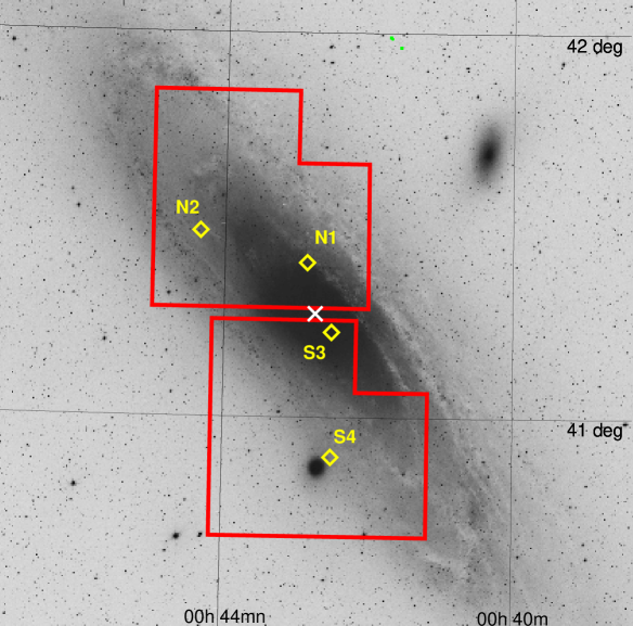
Figure 7: Positions of the four microlensing events projected on M31. The red lines show the contour of the observed fields. Note that S4 lies just next to M32.

PA-99-N1: For this event it has been possible to identify the source on HST archival images. The knowledge of the flux of the unamplified source allows to break the degeneracy between the Einstein crossing time and the impact parameter for which one obtains the values $t_{E}=9.7\pm 0.7$ and $u_{0}=0.057\pm 0.004$. The baseline shows two secondary bumps: they are due to a variable star lying some 3 pixels away from the microlensing variation. The position of this event, $7^{\prime}\,52^{\prime\prime}$ from the center of M31, makes unlikely the hypothesis of bulge-bulge self-lensing. The lens can be either a MACHO (with equal chance in the M31 or the Milky Way halo) or a low mass ($\sim 0.2\,M_{\odot}$) disk star with the source lying in the bulge. The first case is more likely assuming a halo fraction in form of MACHOs above 20%.

PA-99-N2: This variation lies at some $22^{\prime\prime}$ away from the center of M31, therefore is an excellent microlensing MACHO candidate. However, this variation turns out to be almost equally likely to be due to disk–disk self lensing. This light curve is particularly interesting because it shows clear deviations from a Paczyński shape, while remaining achromatic (and unique) as expected for a microlensing event. We recall that this shape is characteristic for variations where the point-like (source and lens) and uniform motion hypothesis hold. After exploring[34] different explanations, it is found that the observations are consistent with an unresolved RGB or AGB star in M31 being microlensed by a binary lens, with a mass ratio of $\sim 1.2\times 10^{-2}$. An analysis of the relative optical depth shows that a halo lens (whose mass is estimated to lie in the range 0.009-32 $M_{\odot}$) is more likely than a stellar lens (with mass in this case expected in the range 0.02-3.6 $M_{\odot}$) provided that the halo mass fraction in form of compact objects is at least around $15\%$.

PA-00-S3: This event is the nearest found so far from the center of M31 ($d=4^{\prime}\,00^{\prime\prime}$). Its extension past in time on MDM data shows no variations. The good sampling along the bump allows to get a rather robust estimation of the Einstein time, $t_{E}=13\pm 4$ days. This value, together with its position, makes the bulge-bulge self-lensing hypothesis the most likely for this event.

PA-00-S4: This event is found far away from the M31 center, but only at $2^{\prime}\,54^{\prime\prime}$ from the center of the dwarf galaxy M32. A detailed analysis[35] shows that the source is likely to be a M31 disk A star, the main evidence being the observed rather blue colour $(R-I)=0.0\pm 0.1$. Given that M32 lies $\sim$ 20 kpc in front of M31, the study of the relative optical depth allows to conclude that the most likely position for the lens is M32.

7 Conclusions

We have presented the results of microlensing survey towards LMC by using the new picture of LMC given by van der Marel et al. [14]. One interesting feature, that clearly emerges in this framework by studying the microlensing signature we expect to find, is an evident near–far asymmetry of the optical depth for lenses located in the LMC halo. Indeed, similarly to the case of M31 [17, 19], and as first pointed out by Gould[36], since the LMC disk is inclined, the optical depth is higher along lines of sight passing through larger portions of the LMC halo. Such an asymmetry is not expected, on the contrary, for a self-lensing population of events. What we show is that, indeed, a spatial asymmetry that goes beyond the one expected from the observational strategy alone, and that is coherent with that expected because of the inclination of the LMC disk, is actually present. With the care suggested by the small number of detected events on which this analysis is based, this can be looked at, as yet observed by Gould[36], as a signature of the presence of an extended halo around LMC.

As already remarked, any spatial asymmetry is not expected for a self-lensing population of events, so that what emerges from this analysis can be considered as an argument to exclude it.

Furthermore, keeping in mind the observation[37] that the timescale distribution of the events and their spatial variation across the LMC disk offers possibilities of identifying the dominant lens population, we have carefully characterized the ensemble of observed events under the hypothesis that all of them do belong to the self-lensing population. Through this analysis we have been able to identify a large subset of events that can not be accounted as part of this population. Again, the small amount of events at disposal does not yet allow us to draw sharp conclusions, although, the various arguments mentioned above are all consistent among them and converge quite clearly in the direction of excluding self-lensing as being the major cause for the events.

Once more observations will be available, as will hopefully be the case with the SuperMacho experiment under way [38], the use of the above outlined methods can bring to a definitive answer to the problem of the location of the MACHOs and thus also to their nature.

As a general outcome of presently available pixel lensing results, we can clearly infer that the detection of microlensing events towards M31 is now established. The open issue to be still explored is the study of the M31 halo fraction in form of MACHOs. With respect to this analysis, the events detected so far are all compatible with stellar lenses, but the MACHO hypothesis is still open, and we recall that the analysis for the INT data is still not concluded (besides a third year data, variations with $\Delta R_{max}>21$ have still to be studied). Once this analysis completed, it is the necessary to “weight” it with an efficiency study of the pipeline of detection before meaningfully comparing its results with the prediction of a Monte Carlo simulation. This should eventually allow us to draw firm conclusions on the halo content in form of MACHO of M31.

Figure 8: Three years data light curves for the 4 POINT-AGAPE microlensing events.

——————————————————————

References

- [1] Paczyński, B. 1986, ApJ 304, 1
- [2] Alcock, C., Allsman, R.A., Alves, D.R., et al. 2000a, ApJ 542, 281
- [3] Lasserre, T. et al. 2000, A&A 355, L39
- [4] Milsztajn, A., & Lasserre, A. 2001, Nucl. Phys. B Proc. Sup. 91,413
- [5] Sahu, K.C. 1994, PASP 106, 942
- [6] Aubourg,E., Palanque-Delabrouille, N., Salati, P., et al. 1999, A&A 347, 850
- [7] Evans N. W., Gyuk, G., Turner M. S. & Binney J. J. 1998, ApJ 501, L45
- [8] Zhao, H.S., & Evans, N.W. 2000, ApJ 545, L35
- [9] Jetzer, Ph., Mancini, L. & Scarpetta, G. 2002, A&A 393, 129
- [10] Mancini, L., Calchi Novati, S., Jetzer, Ph. & Scarpetta G. 2004, to appear in A&A
- [11] Alcock, C., Allsman, R.A., Alves, D.R., et al. 2000b, ApJ 541, 270
- [12] Alcock, C., Allsman, R.A., Alves, D.R., et al. 2001b, ApJ 552, 259
- [13] Alcock, C., Allsman, R.A., Alves, D.R., et al. 2001c, ApJ 552, 582
- [14] van der Marel, R.P., & Cioni, M.R. 2001, AJ 122, 1807
- [15] van der Marel, R.P. 2001, AJ 122, 1827
- [16] van der Marel, R.P. , Alves, D.R., Hardy, E., & Suntzeff, N.B. 2002, AJ 124, 2639
- [17] A. P. Crotts, A.P. 1992, ApJ 399, L43
- [18] Baillon, P., Bouquet, A., Giraud-Héraud, Y., & Kaplan, J. 1993, A&A 277, 1
- [19] Jetzer, Ph. 1994, A&A 286, 426
- [20] Baltz, E. et al., astro-ph/0310845
- [21] Ansari, R. et al. 1997, A&A 324, 843
- [22] Ansari, R. et al. 1999, A&A 344, L49
- [23] Tomaney, A. & Crotts, A. 1996, AJ 112, 2872
- [24] Calchi Novati, S. et al. 2002, A&A 381, 848
- [25] Calchi Novati, S. et al. 2003, A&A 405, 851
- [26] Aurière, M. et al. 2001, ApJ 553, L137
- [27] Paulin-Henriksson, S. et al. 2003, A&A 405, 15
- [28] Riffeser, A. et al. 2001, A&A 379, 362
- [29] Riffeser, A. et al. 2003, ApJ 599, L17
- [30] de Jong, J. et al., astro-ph/0307072
- [31] Gyuk, G., Dalal, N. & Griest, K. 2000, ApJ 535, 90
- [32] De Rújula, A., Jetzer, Ph., & Massó, E. 1991, MNRAS 250, 348
- [33] Chabrier, G. 2001, ApJ 554, 1274
- [34] An, J. et al., ApJ in press (astro-ph/0310457)
- [35] Paulin-Henriksson, S. et al. 2002, ApJ 576, L121
- [36] Gould, A. 1993, ApJ 404, 451
- [37] Evans, N.W., & Kerins, E. 2000, ApJ 529, 917
- [38] Stubbs, C. W., Rest, A., Miceli, A., et al. 2002, BAAS 201, #78.07