Testing cosmological models and understanding cosmological parameter determinations with metaparameters

Abstract

Cosmological parameters affect observables in physically distinct ways. For example, the baryon density, $\omega_{b}$, affects the ionization history and also the pressure of the pre-recombination fluid. To investigate the relative importance of different physical effects to the determination of $\omega_{b}$, and to test the cosmological model, we artificially split $\omega_{b}$ into two ‘metaparameters’: $\omega_{be}$ which controls the ionization history and $\omega_{bp}$ which plays the role of $\omega_{b}$ for everything else. In our demonstration of the technique we find $\omega_{b}=.0229\pm.0012$ (with no parameter splitting), $\omega_{bp}=.0238\pm.0021$, $\omega_{be}=.0150\pm.0034$ and $\omega_{bp}-\omega_{be}=.0088\pm.0039$.

1. Introduction

As predicted (Spergel, 1995; Knox, 1995; Jungman et al., 1996), observations of the cosmic microwave background (CMB) anisotropies (e.g. Kuo et al. (2004); Bennett et al. (2003); Readhead et al. (2004)) have provided very tight constraints on cosmological parameters (e.g. Spergel et al. (2003); Goldstein et al. (2003); Rebolo et al. (2004)). These constraints are possible because the statistical properties are sufficiently rich and, given a model, can be calculated with very high accuracy (e.g. Hu & Dodelson (2002)).

One must bear in mind though that these determinations are highly indirect and model-dependent. It is therefore useful to have tools for testing the model, and for gaining better understanding of the particular physical processes important for a given constraint. Toward these ends, we explore use of cosmological ‘metaparameters’.

A given parameter, $x$, may lead to observational consequences through more than one distinct physical effect. Such a parameter can be split into more than one metaparameter, $x_{a}$, $x_{b}$, $x_{c}$, … each of which controls a different physical effect. This approach to data analysis has been developed independently and applied recently by Zhang et al. (2003) who call it ‘parameter splitting.’ Their motivation was to marginalize over physical effects that could not be calculated with sufficient accuracy. One can also use the split into metaparameters to test the model (by checking if $x_{a}=x_{b}$ to within errors), and to understand where the constraints are coming from (by comparing $\sigma(x_{a})$ to $\sigma(x_{b})$).

In this paper we explore one example of a split into cosmological metaparameters. In particular, we split the baryon density into two parameters: one that controls the ionization history, $\omega_{be}$, and one that controls the inertia of the pre-recombination baryon-photon fluid, $\omega_{bp}$. In section 2 we describe the dependence of the angular power spectrum on these two variables. In section 3 we briefly describe our calculations. In section 4 we show and discuss our results. Finally, in section 5 we conclude.

2. Dependence of $C_{l}$ on $\omega_{be}$ and $\omega_{bp}$

The baryon density affects the evolution of CMB temperature anisotropies in two distinct ways. First, in the pre-recombination plasma, the higher the baryon density, the higher the inertia of the fluid due to the baryon’s mass. Second, the ratio of baryons to photons determines the history of the number density of free electrons (prior to reionization).

These two different physical effects, one related to the baryon’s mass and one related to the large Thomson cross section of the electrons that charge-balance the baryons, lead to different observational consequences. They therefore lead to two different ways to determine the baryon density.

We can study these effects separately by splitting $\omega_{b}\equiv\Omega_{b}h^{2}$ into what we will call $\omega_{be}$ and $\omega_{bp}$ where the $e$ indicates electron and the $p$ stands for pressure. Operationally, we calculate the mean number density of electrons, $n_{e}$, assuming $\omega_{b}=\omega_{be}$, using the recombination routine RECfast (Seager et al., 1999). Then we calculate $C_{l}$ using CMBfast (Seljak & Zaldarriaga, 1996) with $\omega_{b}=\omega_{bp}$ and the $n_{e}(z)$ from RECfast.

2.1. Dependence on $\omega_{bp}$

The response of $C_{l}$ to the two baryon densities can be seen in Fig. 1. First we concentrate on the multiple effects of varying $\omega_{bp}$. Decreasing $\omega_{bp}$ leads to three different physical effects: sound speed increase, acoustic oscillation zero-point shift, and reduction in ‘baryon drag’. We briefly review the effects here though they are all discussed at length in the review by Hu & Dodelson (2002).

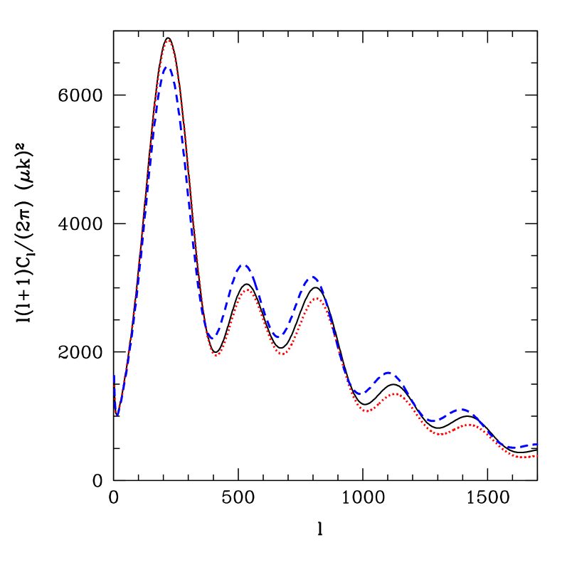
Figure 1.— Dependence of $C_{l}$ on the metaparameters. Solid curve is $C_{l}$ for the fiducial model with $\omega_{bp}=\omega_{be}=0.023$. Dashed (dotted) curve is $C_{l}$ for fiducial model parameters except for $\omega_{bp}=0.018$ ($\omega_{be}=0.018$). The fiducial model is a typical sample from the MCMC chain of our six-parameter model space constrained by the WMAPext dataset.

Adding non-relativistic baryons decreases the sound speed of the fluid, given by

$$c_{s}={1\over\sqrt{3(1+R)}}$$ (1)

where $R\equiv 3\rho_{b}/\rho_{\gamma}$. Reducing $\omega_{bp}$ decreases $R$ and therefore increases the sound speed, causing the oscillation pattern to shift slightly to lower $l$.

In the absence of baryons, if the gravitational potential $\Psi$ is constant then the effective temperature, $\Theta_{0}+\Psi$, oscillates about zero; that is, the competing effects of pressure and gravity cancel when $\Theta_{0}=-\Psi$. Adding baryons reduces the pressure, meaning the baryons must collapse further into a potential well before gravity and pressure balance. The zero point shifts to $\Theta_{0}=-(1+R)\Psi$ and therefore $\Theta_{0}+\Psi$ oscillates about $-R\Psi$. The offset enhances odd peaks (for which the effective temperature is positive in potential hills and therefore $-R\Psi$ is a boost) and suppresses even peaks (for which the effective temperature is negative in potential wells). Decreasing $\omega_{bp}$ therefore suppresses odd peaks and enhances even peaks.

In the above paragraph we assumed a constant $\Psi$ which is a good approximation for the matter-dominated era, but not for radiation domination. For modes that enter during radiation domination, pressure resists transport of material into the potential well, causing the potential to decay as expansion dilutes the over-density. Thus for modes that entered early during radiation domination, by the time of last-scattering the gravitational potential is insignificant and the oscillation is about $\Theta_{0}=0$; there is no offset to the oscillations and therefore no modulation of the even and odd peak heights.

At smaller scales, the dominant effect of a reduction of $\omega_{bp}$ is a reduction in ‘baryon drag’. The baryon drag effect can be thought of as due to the increasing value of $R$ over time. As $R$ increases in time, the sound speed decreases, so the oscillation frequency decreases. Since energy/frequency of an oscillator is an adiabatic invariant, this decrease in frequency is matched by a decrease in oscillation amplitude. Since $\dot{R}\propto R$, decreasing $\omega_{bp}$ decreases the amount of baryon drag, and the power is enhanced. Note that the baryon drag effect is is distinct from the photon diffusion we discuss in the next subsection. This distinction is clear from the fact that there is baryon drag even in the tight coupling limit.

The scale of matter radiation equality projected to today comes out at $l_{\rm eq}\simeq 170$ (Knox et al., 2001) and therefore the first peak entered slightly before matter-radiation equality. Both effects (zero-point offset and baryon drag) are important for the first peak and partially cancel each other out. For the second peak, the effects add so that decreasing $\omega_{bp}$ enhances power. For the third peak, having entered earlier during radiation domination, the offset effect is sub-dominant to baryon drag so power is enhanced.

2.2. Dependence on $\omega_{be}$

Even prior to recombination, the mean free path due to Thomson scattering is non-zero. Photons thus diffuse, damping the power spectrum on small scales. The comoving damping length is given by the distance the photons can random walk by the time of last scattering. Decreasing $\omega_{be}$ decreases the number density of baryons, $n_{b}$, and therefore, for fixed ionization fraction, the number of free electrons, $n_{e}=x_{e}n_{b}$. The resulting increase in mean free path increases the damping length.

The effect of varying $\omega_{be}$ on the damping length is complicated by the fact that decreasing $\omega_{be}$ increases the number of photons per baryon and therefore alters $x_{e}(z)$. More photons per baryon delays recombination. This means that at a given time more atoms are ionized (tending to decrease the damping scale), and it also means a delay in recombination giving more time for the random walking (tending to increase the damping scale). Hu & White (1997) found that the net result is that the damping length scale is roughly proportional to $\omega_{b}^{-1/4}$. Reducing $\omega_{be}$ therefore increases the damping length, leading to the increased suppression for the dotted curve seen in Fig. 1.

The damping length projected from the last-scattering surface to here, a comoving distance $D$ away, gives rise to an angular scale, $\pi/l_{D}$. Below we use $l_{D}$ as a function of cosmological parameters as written in Hu et al. (2001) with the difference that we numerically evaluate the redshift of last-scattering, $z_{*}$, as the peak of the visibility function, and replace $\omega_{b}$ with $\omega_{be}$.

3. Calculating the Likelihood

What we want to know is, given the data and any other assumptions we make about the world, what is the probability distribution of the parameters? This posterior probability distribution can be calculated by use of Bayes’ theorem which states:

$$P({\vec{\theta}}|d)\propto P(d|{\vec{\theta}})P_{\rm prior}({\vec{\theta}})\,.$$ (2)

where $d$ refers to data and the proportionality constant is chosen to ensure $\int P({\vec{\theta}}|d)d{\vec{\theta}}=1$. With a uniform prior this simply reduces to $P({\vec{\theta}}|d)\propto P(d|{\vec{\theta}})$. This probability of the data given the parameters is, when thought of as a function of the parameters, called the likelihood, ${\cal L}({\vec{\theta}})$.

Often we are interested in the posterior probability distribution for one or two parameters alone. This marginalized posterior is given by integrating over the other parameters. For example:

$$P(\theta_{1},\theta_{2}|d)=\int\Pi_{i=3}^{n}d\theta_{i}{\cal L}(\vec{\theta})P_{\rm prior}(\vec{\theta})$$ (3)

where $n$ is the number of parameters. We use the prior to incorporate non–CMB information such as that the redshift of reionization must be greater than 6.0 (Becker et al., 2001).

In the following subsections we discuss first how we evaluate the likelihood function at a single point and then how we evaluate it over a large parameter space and produce marginalized posterior distributions.

3.1. Likelihood evaluation

The first step to likelihood evaluation is to calculate the angular power spectrum, $C_{l}$, for the cosmological model. To do this we use CMBfast. Despite its speed advantages we do not use the Davis Anisotropy Shortcut (DASh; Kaplinghat et al. (2002)) since the split $\omega_{b}$ modifications were easier with CMBfast than with DASh.

Once $C_{l}$ is calculated we evaluate the likelihood given the WMAP data with the subroutine available at the LAMBDA data archive. For CBI and ACBAR we use the offset log-normal approximation of the likelihood (Bond et al., 2000). The likelihood given all these data together (referred to as the WMAPext dataset in Spergel et al. (2003)) is given by the product of the individual likelihoods.

We do not use the most recent release of CBI data (Readhead et al., 2004), nor the VSA data (Dickinson et al., 2004). We have used the older release (Pearson et al., 2003) for ease of comparison with results in Spergel et al. (2003). The new CBI data (Readhead et al., 2004) and the VSA data are consistent with the old CBI data, WMAP and ACBAR (Dickinson et al., 2004; Rebolo et al., 2004).

3.2. Exploring the Parameter Space

We explore several parameter spaces. What we refer to as the six-parameter model has six cosmological parameters (the baryon density, the cold dark matter density, the scalar primordial power spectrum amplitude at $k=0.05\,{\rm Mpc}^{-1}$, $n_{S}$, the redshift of reionization and $\Omega_{\Lambda}$) and a calibration parameter for each of CBI and ACBAR. The split model is the same except the baryon density, $\omega_{b}$, is replaced with $\omega_{be}$ and $\omega_{bp}$.

We explore the parameter space by producing a Monte Carlo Markov Chain (MCMC) via the Metropolis–Hastings algorithm as described in Christensen et al. (2001). Our procedure is the same as in Chu et al. (2003) except for some changes to the adaptive phase of the sampling, during which the generating function is determined. Our WMAPext chain for the six-parameter model space has 80,000 samples and the WMAPext chain for the seven-parameter split model space has 130,000 samples.

4. Results

We now examine how the likelihood function changes as the parameter space is expanded to non-zero $\omega_{bp}-\omega_{be}$.

4.1. Constraints on $\omega_{be}$ and $\omega_{bp}$

In Fig. 2we see the resulting constraints on $\omega_{b}$ (assuming no splitting), $\omega_{be}$ and $\omega_{bp}$. Note that, without splitting, we find $\omega_{b}=0.0229\pm 0.0012$ which reproduces the result from Spergel et al. (2003) of $0.023\pm 0.001$ for the same model space and dataset.

For the unsplit parameter there is a tension between increasing the damping length (which occurs by lowering $\omega_{b}$) and increasing inertial effects (which occurs by raising $\omega_{b}$). This tension only becomes evident once we split the parameter and see that $\omega_{be}$ drifts downward and $\omega_{bp}$ drifts slightly upward.

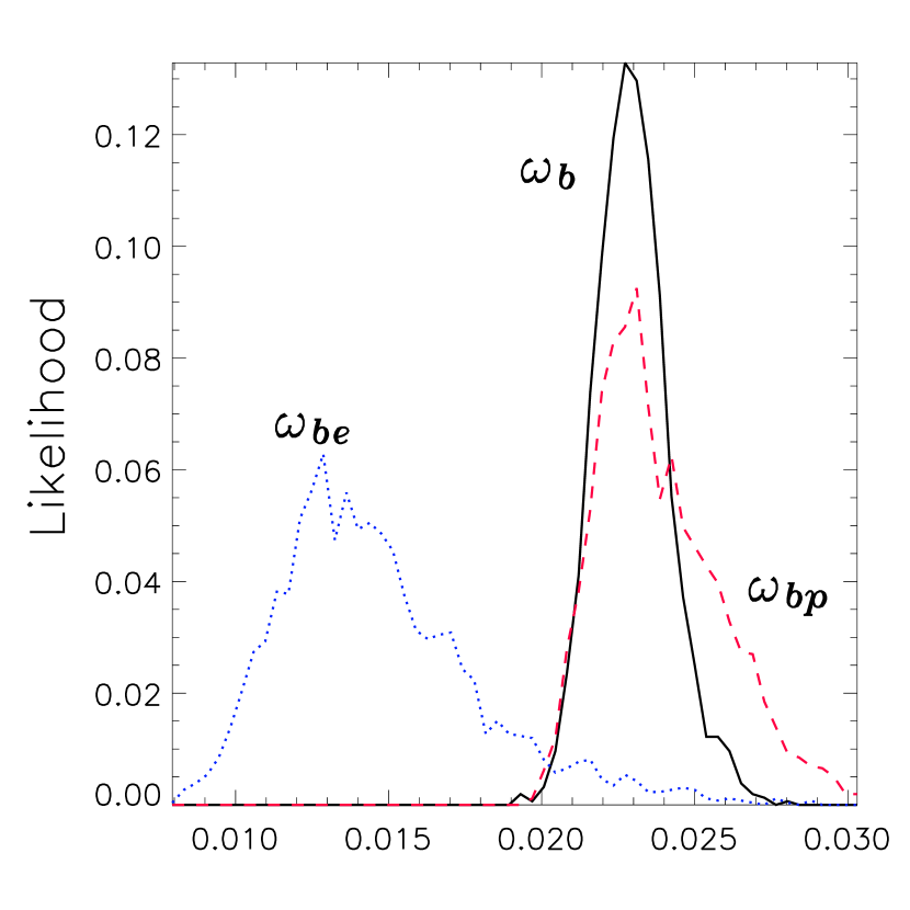
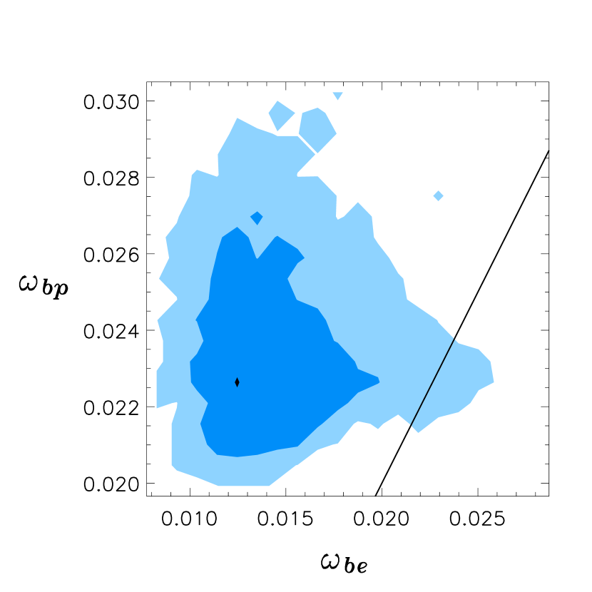
Figure 2.— Left panel: One-dimensional marginalized likelihoods of $\omega_{b}$ (assuming no parameter splitting), $\omega_{be}$ and $\omega_{bp}$. Right panel: Two-dimensional marginalized likelihood of $\omega_{bp}$ vs. $\omega_{be}$. Dark (light) shaded region is where the likelihood is down by less than a factor of $\exp(-2.3/2)$ ($\exp(-6.17/2)$) from its maximum value. The line is $\omega_{bp}=\omega_{be}$.

In Fig. 3 we see why the data tend to favor lower $\omega_{be}$: it improves the fit in the damping tail region. Model fits with the six-parameter model lead to excess model power at higher $l$. Allowing $\omega_{be}$ to vary independently from $\omega_{bp}$ gives the necessary freedom to eliminate this excess and improve the over all fit. The tendency for $\omega_{bp}$ to drift upward, seen in Fig. 2, has indirect causes as we explain in the next subsection.

The excess small-scale power of the six-parameter model fits is also what causes the slight preference of the data for $dn_{S}/d\ln k<0$. Spergel et al. (2003) find for WMAPext that $dn_{S}/d\ln k=-0.055\pm 0.038$. This extension by splitting $\omega_{b}$ actually leads to somewhat better agreement with the data than the extension to $dn_{S}/d\ln k\neq 0$. We find the maximum likelihood improves by a factor of 8.2 with the extension to split $\omega_{b}$ and 2.8 with the extension to $dn_{S}/d\ln k\neq 0$.

In the right panel of Fig. 2 we see the constraints in the $\omega_{bp}$-$\omega_{be}$ plane. The straight line is the physical subspace, $\omega_{bp}=\omega_{be}$. How significant is the deviation from the physical subspace? We find $\omega_{bp}-\omega_{be}=0.0088\pm 0.0039$, a 2.3$\sigma$ difference from zero. The difference from zero could simply be a statistical fluctuation, it could be caused by systematic error in one or more of the experiments, or it could be that the six-parameter model does not adequately describe reality. The discrepancy is not strong enough to rule out the first option.

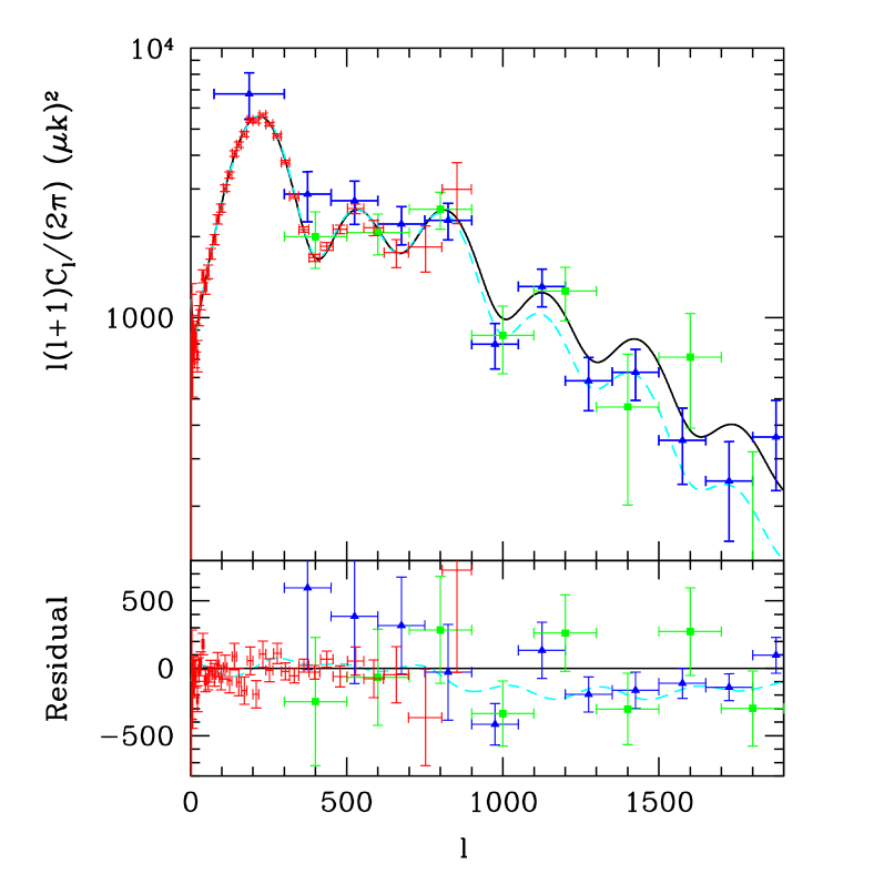
Figure 3.— Top panel: CMB constraints on the power spectrum, the fiducial six-parameter model, and an improved fit that comes from allowing $\omega_{bp}\neq\omega_{be}$. Bottom panel: Same as above, but with the fiducial six-parameter model subtracted.

4.2. Constraints on other parameters

Splitting $\omega_{b}$ alters the constraints on other parameters too. To gain a better understanding of the model dependence we now examine how constraints on $\tau$, $n_{S}$ and $\omega_{m}$ change.

In the six-parameter model there is a tension between the value of $\tau$ that best fits the $C_{l}^{TT}$ data ($\tau=0$) and the larger value which best fits the $C_{l}^{TE}$ data. Allowing extra freedom in the damping tail, by splitting $\omega_{b}$, makes it possible for a higher $\tau$ to be consistent with the $C_{l}^{TT}$ data as can be seen in Fig. 4. Increasing $n_{S}$ can compensate for increased $\tau$, but too large an $n_{S}$ leads to too much power on small scales. Extra damping from decreased $\omega_{be}$ compensates for this excess power. Further, increased $n_{S}$ increases the ratio of the 2nd peak height to first peak height, and therefore $\omega_{bp}$ increases to compensate.

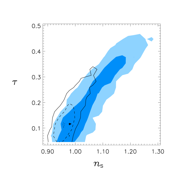
Figure 4.— Two- and one-dimensional marginalized likelihoods. Left panel: The dashed (solid) line is where the likelihood of $n_{s}$ and $\tau$ given the WMAPext dataset assuming the six-parameter model is down by a factor of $\exp(-2.3/2)$ ($\exp(-6.17/2)$) from its maximum value. Shading indicates the same regions, but for the split model space. Middle and right panels: One-dimensional marginalized likelihoods of $\omega_{m}$ and $l_{D}$ given the WMAPext dataset. Solid lines are for the six-parameter model space and dashed lines are for the split model space.

We also see in Fig. 4 that the likelihood function of $\omega_{m}$ has broadened some toward higher values. Spergel et al. (2003) claim that the constraint on $\omega_{m}$ is largely coming from the rise to the first peak and how the shape of the spectrum in this region is influenced by the early integrated Sachs-Wolfe (ISW) effect. The amount of fluctuation power from the early ISW effect depends on the ratio of matter energy density to radiation energy density at last scattering. We see from our split model chains that models with higher $z_{*}$ also tend to have higher $\omega_{m}$, as they must to keep $\rho_{m}/\rho_{z}$ at $z_{*}$ nearly fixed.

4.3. Benefits of measuring the damping tail

Measuring the damping tail region of the spectrum to high precision will be very valuable. In the context of the six parameter model it will allow for much tighter constraints on $\omega_{b}$, $\omega_{m}$ and $n_{S}$. Whereas WMAP will measure out to about $l=500$ with cosmic variance precision, Planck (Tauber, 2001) will measure out to about $l=2000$ with cosmic variance precision, reducing the errors on the above parameters by factors of 6, 5 and 6 respectively (Eisenstein et al., 1999).

Perhaps more importantly, measuring the damping tail will allow more stringent tests of the model. The six-parameter model, calibrated with measurements at larger angular scales, makes tight predictions for the damping tail region. For example, the damping scale $l_{D}$, is very tightly constrained with the WMAPext data given the six-parameter model, as can be seen in Fig. 4. But these tight constraints are not because we have measured the damping tail well. They are due to the fact that the parameters controlling the damping tail region can be determined well at larger angular scales.

With the split model we weaken this connection between the acoustic region and the damping region. As a result, the constraints on $l_{D}$ weaken considerably as seen in Fig. 4 . Future high precision measurements of the damping tail will be able to determine $l_{D}$ with high accuracy. Then the prediction for $l_{D}$, given the six-parameter model and acoustic region data, can be compared with $l_{D}$ inferred from the damping region, allowing for a strong test of the model.

Current measurements of the damping tail are already playing an important role in testing the six-parameter model. ACBAR and CBI do reduce the allowed region of the six-dimensional parameter space some, but mostly serve to confirm the WMAP predictions (albeit with slightly lower power). Once we allow for the parameter split, ACBAR and CBI place significant extra constraints on the parameter space. For example, constraints on the split $\omega_{b}$ model from the WMAP data mean that ${\cal C}_{1400}=805\pm 169$ (where ${\cal C}_{l}\equiv l(l+1)C_{l}/(2\pi)$). Inclusion of the ACBAR and CBI data change this to $695\pm 79$, reducing the uncertainty by a factor of two. In contrast, without the $\omega_{b}$ split, adding ACBAR and CBI only reduces the ${\cal C}_{1400}$ error by 30%.

5. Conclusions

We have introduced the creation of cosmological metaparameters as a tool for exploring the powerful, complicated, model-dependent constraints on cosmological parameters possible with measurements of CMB anisotropy. Such an exploration is useful for gaining a physical understanding of the origin of the constraints and for testing the consistency of the model. We see, as expected, $\omega_{b}$ is mostly constrained via the observable consequences of its effect on the inertia of the pre-recombination plasma. Electron-scattering effects play a sub-dominant role. Determinations of $\omega_{b}$ from the two different effects differ by 2.3$\sigma$; i.e., they are marginally consistent with each other.

It is amazing that a model with only six parameters can provide such a good fit to the WMAPext dataset. With the assumption of this model, fairly tight constraints are possible on parameters such as $n_{S}$ and $\omega_{b}$. We see though, as others have seen (Tegmark et al., 2004), that extending the model space by just one parameter can greatly broaden the constraints on other parameters. Interpretation of CMB constraints on cosmological parameters must be done with care.

In particular we have seen that the modeling of processes that affect the damping tail region of the spectrum can greatly loosen bounds on $n_{S}$ and $\tau$. Other (physical) parameter extensions that would affect the damping tail region are running, and a time-varying fine structure constant (Kaplinghat et al., 1999). Measurement of the damping tail with great precision, such as will be done by Planck, will dramatically decrease the sensitivity to modeling uncertainty and provide stringent consistency tests.

References

- Becker et al. (2001) Becker, R. H., Fan, X., White, R. L., Strauss, M. A., Narayanan, V. K., Lupton, R. H., Gunn, J. E., Annis, J., Bahcall, N. A., Brinkmann, J., Connolly, A. J., Csabai, I. ., Czarapata, P. C., Doi, M., Heckman, T. M., Hennessy, G. S., Ivezić, Ž., Knapp, G. R., Lamb, D. Q., McKay, T. A., Munn, J. A., Nash, T., Nichol, R., Pier, J. R., Richards, G. T., Schneider, D. P., Stoughton, C., Szalay, A. S., Thakar, A. R., & York, D. G. 2001, AJ, 122, 2850
- Bennett et al. (2003) Bennett, C. L., Halpern, M., Hinshaw, G., Jarosik, N., Kogut, A., Limon, M., Meyer, S. S., Page, L., Spergel, D. N., Tucker, G. S., Wollack, E., Wright, E. L., Barnes, C., Greason, M. R., Hill, R. S., Komatsu, E., Nolta, M. R., Odegard, N., Peiris, H. V., Verde, L., & Weiland, J. L. 2003, ApJS, 148, 1
- Bond et al. (2000) Bond, J. R., Jaffe, A. H., & Knox, L. 2000, ApJ, 533, 19
- Christensen et al. (2001) Christensen, N., Meyer, R., Knox, L., & Luey, B. 2001, Classical Quantum Gravity, 18, 2677
- Chu et al. (2003) Chu, M., Kaplinghat, M., & Knox, L. 2003, ApJ, 596, 725
- Dickinson et al. (2004) Dickinson, C., Battye, R. A., Cleary, K., Davies, R. D., Davis, R. J., Genova-Santos, R., Grainge, K., Gutierrez, C. M., Hafez, Y. A., Hobson, M. P., Jones, M. E., Kneissl, R., Lancaster, K., Lasenby, A., Leahy, J. P., Maisinger, K., Odman, C., Pooley, G., Rajguru, N., Rebolo, R., Rubino-Martin, J. A., Saunders, R. D. E., Savage, R. S., Scaife, A., Scott, P. F., Slosar, A., Molina, P. S., Taylor, A. C., Titterington, D., Waldram, E., Watson, R. A., & Wilkinson, A. 2004, ArXiv Astrophysics e-prints
- Eisenstein et al. (1999) Eisenstein, D. J., Hu, W., & Tegmark, M. 1999, ApJ, 518, 2
- Goldstein et al. (2003) Goldstein, J. H., Ade, P. A. R., Bock, J. J., Bond, J. R., Cantalupo, C., Contaldi, C. R., Daub, M. D., Holzapfel, W. L., Kuo, C., Lange, A. E., Lueker, M., Newcomb, M., Peterson, J. B., Pogosyan, D., Ruhl, J. E., Runyan, M. C., & Torbet, E. 2003, ApJ, 599, 773
- Hu & Dodelson (2002) Hu, W. & Dodelson, S. 2002, ARA&A, 40, 171
- Hu et al. (2001) Hu, W., Fukugita, M., Zaldarriaga, M., & Tegmark, M. 2001, ApJ, 549, 669
- Hu & White (1997) Hu, W. & White, M. 1997, ApJ, 479, 568
- Jungman et al. (1996) Jungman, G., Kamionkowski, M., Kosowsky, A., & Spergel, D. N. 1996, Phys. Rev. D, 54, 1332
- Kaplinghat et al. (2002) Kaplinghat, M., Knox, L., & Skordis, C. 2002, ApJ, 578, 665, astro-ph/0203413
- Kaplinghat et al. (1999) Kaplinghat, M., Scherrer, R. J., & Turner, M. S. 1999, Phys. Rev. D, 60, 023516
- Knox (1995) Knox, L. 1995, Phys. Rev. D, 52, 4307
- Knox et al. (2001) Knox, L., Christensen, N., & Skordis, C. 2001, ApJ, 563, L95
- Kuo et al. (2004) Kuo, C. L., Ade, P. A. R., Bock, J. J., Cantalupo, C., Daub, M. D., Goldstein, J., Holzapfel, W. L., Lange, A. E., Lueker, M., Newcomb, M., Peterson, J. B., Ruhl, J., Runyan, M. C., & Torbet, E. 2004, ApJ, 600, 32
- Pearson et al. (2003) Pearson, T. J., Mason, B. S., Readhead, A. C. S., Shepherd, M. C., Sievers, J. L., Udomprasert, P. S., Cartwright, J. K., Farmer, A. J., Padin, S., Myers, S. T., Bond, J. R., Contaldi, C. R., Pen, U.-L., Prunet, S., Pogosyan, D., Carlstrom, J. E., Kovac, J., Leitch, E. M., Pryke, C., Halverson, N. W., Holzapfel, W. L., Altamirano, P., Bronfman, L., Casassus, S., May, J., & Joy, M. 2003, ApJ, 591, 556
- Readhead et al. (2004) Readhead, A. C. S., Mason, B. S., Contaldi, C. R., Pearson, T. J., Bond, J. R., Myers, S. T., Padin, S., Sievers, J. L., Cartwright, J. K., Shepherd, M. C., Pogosyan, D., Prunet, S., Altamirano, P., Bustos, R., Bronfman, L., Casassus, S., Holzapfel, W. L., May, J., Pen, U. ., Torres, S., & Udomprasert, P. S. 2004, ArXiv Astrophysics e-prints
- Rebolo et al. (2004) Rebolo, R., Battye, R. A., Carreira, P., Cleary, K., Davies, R. D., Davis, R. J., Dickinson, C., Genova-Santos, R., Grainge, K., Gutirrez, C. M., Hafez, Y. A., Hobson, M. P., Jones, M. E., Kneissl, R., Lancaster, K., Lasenby, A., Leahy, J. P., Maisinger, K., Pooley, G. G., Rajguru, N., Rubino-Martin, J. A., Saunders, R. D. E., Savage, R. S., Scaife, A., Scott, P. F., Slosar, A., Molina, P. S., Taylor, A. C., Titterington, D., Waldram, E., Watson, R. A., & Wilkinson, A. 2004, ArXiv Astrophysics e-prints
- Seager et al. (1999) Seager, S., Sasselov, D. D., & Scott, D. 1999, ApJ, 523, L1
- Seljak & Zaldarriaga (1996) Seljak, U. & Zaldarriaga, M. 1996, ApJ, 469, 437
- Spergel (1995) Spergel, D. N. 1995, in AIP Conf. Proc. 336: Dark Matter, 457–+
- Spergel et al. (2003) Spergel, D. N. et al. 2003, astro-ph/0302209
- Tauber (2001) Tauber, J. A. 2001, in IAU Symposium, 493–+
- Tegmark et al. (2004) Tegmark, M., Strauss, M. A., Blanton, M. R., Abazajian, K., Dodelson, S., Sandvik, H., Wang, X., Weinberg, D. H., Zehavi, I., Bahcall, N. A., Hoyle, F., Schlegel, D., Scoccimarro, R., Vogeley, M. S., Berlind, A., Budavari, T., Connolly, A., Eisenstein, D. J., Finkbeiner, D., Frieman, J. A., Gunn, J. E., Hui, L., Jain, B., Johnston, D., Kent, S., Lin, H., Nakajima, R., Nichol, R. C., Ostriker, J. P., Pope, A., Scranton, R., Seljak, U., Sheth, R. K., Stebbins, A., Szalay, A. S., Szapudi, I., Xu, Y., Annis, J., Brinkmann, J., Burles, S., Castander, F. J., Csabai, I., Loveday, J., Doi, M., Fukugita, M., Gillespie, B., Hennessy, G., Hogg, D. W., Ivezić, Ž., Knapp, G. R., Lamb, D. Q., Lee, B. C., Lupton, R. H., McKay, T. A., Kunszt, P., Munn, J. A., O’Connell, L., Peoples, J., Pier, J. R., Richmond, M., Rockosi, C., Schneider, D. P., Stoughton, C., Tucker, D. L., vanden Berk, D. E., Yanny, B., & York, D. G. 2004, Phys. Rev. D, 69, 103501
- Zhang et al. (2003) Zhang, J., Hui, L., & Stebbins, A. 2003, ArXiv Astrophysics e-prints