The slowly expanding envelope of CRL618 probed with HC₃N rotational ladders

Abstract

Lines from HC₃N and isotopic substituted species in ground and vibrationally excited states produce crowded millimeter and submillimeter wave spectra in the C-rich protoplanetary nebula CRL618. The complete sequence of HC₃N rotational lines from J=9–8 to J=30–29 has been observed with the IRAM 30m telescope toward this object. Lines from a total of 15 different vibrational states (including the fundamental), with energies up to 1100 cm^-1, have been detected for the main HC₃N isotopomer. In addition, the CSO telescope has been used to complement this study in the range J=31–30 to J=39–38, with detections in five of these states, all of them below 700 cm^-1. Only the rotational lines of HC₃N, in its ground vibrational state, display evidence of the well known CRL618 high velocity velocity outflow. Vibrationally excited HC₃N rotational lines exhibit P-Cygni profiles at 3 mm, evolving to pure emission lineshapes at shorter wavelengths. This evolution of the line profile shows little dependence on the vibrational state from which they rotational lines arise. The absorption features are formed against the continuum emission, which has been successfully characterized in this work due to the large frequency coverage. The fluxes range from 1.75 to 3.4 Jy in the frequency range 90 to 240 GHz. These values translate to an effective continuum source with a size between 0.22” and 0.27” and effective temperature at 200 GHz ranging from 3900 to 6400 K with spectral index between -1.15 and -1.12. We have made an effort to simultaneously fit a representative set of observed HC₃N lines through a model for an expanding shell around the central star and its associated HII region assuming that LTE prevails for HC₃N. The simulations show that the inner slowly expanding envelope has expansion and turbulence velocities of $\sim$ 5-18 kms^-1 and $\sim$ 3.5 kms^-1 respectively, and that it is possibly elongated. Its inclination with respect to the line of sight has also been explored. The HC₃N column density in front of the the continuum source has been determined by comparing the output of an array of models to the data. The best fits are obtained for column densities in the range 2.0-3.5$\cdot$10¹⁷ cm^-2, consistent with previous estimates from ISO data, and T_K in the range 250 to 275 K, in very good agreement with estimates made from the same ISO data.

1 Introduction

CRL 618 is probably the best example of a C-rich protoplanetary nebula (PPNe) with a thick molecular envelope (Bujarrabal et al. 1988) surrounding a B0 star and an ultracompact HII region from which UV radiation impinges on the envelope. Its distance of 1.7 kpc makes this object one of the best suited sources for studying the evolutionary stages from the Asymptotic Giant Branch (AGB) to planetary nebulae (Herpin et al. 2002). The brightening of the HII region in the 1970s (Kwok & Feldman 1981; Martín-Pintado et al. 1993) and the discovery of high velocity molecular winds (HVMW) with velocities up to 200 kms^-1 (Cernicharo et al. 1989) illustrate the rapid evolution of the central star and its influence on the circumstellar ejected material. From observations of molecular gas at arcsecs resolution, the high velocity molecular outflow and the slowly expanding envelope have been resolved and precisely located around the ultracompact HII region (Neri et al. 1992, Cox et al., 2003, Sánchez-Contreras & Sahai, 2004).

The recent discovery of the polyynes HC₄H and HC₆H and of benzene (C₆H₆), the first aromatic molecule detected outside the solar system, in CRL618 (Cernicharo et al., 2001a,b), emphasizes the fact that the copious mass ejection, toward the end of the AGB phase, and the related shock and UV driven chemistry, make the C-rich nebulae of this type very efficient factories of organic molecules (see detailed chemical models for this object in Cernicharo 2004). Small hydrocarbons and pure carbon chains are formed and they can in turn be the small nuclei from which larger C-rich molecules, such as the Poli-Aromatic Hydrocarbons (PAHs) can be built. These molecules are proposed as responsible for the observed emission labeled as Unidentified Infrared Bands (UIBs).

In order to draw the clearest picture of the chemical composition, structure and dynamics of CRL618, it is necessary to perform complete line surveys in those regions of the electromagnetic spectrum where most molecules do emit. One of these line surveys has been carried out by us at millimeter wavelengths with the IRAM 30m telescope (Cernicharo et al., in prep.). One of the most important features seen in the survey is the presence of clusters of lines with a frequency separation of $\simeq$ 9 GHz, corresponding to rotational transitions in the ground and vibrationally excited states of HC₃N. This molecule belongs to the cyanopolyynes, HC_2n+1N, an important group of interstellar molecules (detected in space up to 2n+1=11, Bell et al. 1997). Because of the relatively low-energy of their bending modes, they can be found in space in many vibrationally excited states. As an example Wyrowski et al. (1999) detected HC₃N in eleven vibrationally excited states with energies up to 1100 cm^-1 toward the ultracompact HII region G10.47+0.03. The small frequency spacings of the HC₃N rotational transitions make this molecule an interesting tool to probe the physical conditions of molecular gas in C-rich circumstellar shells such as in CRL618. The HC₃N line profiles in this object show the interesting behavior of evolving, with frequency, from P-Cygni to normal emission. This is presented and analyzed in this paper using a model, under LTE, for an expanding envelope of azimuthally symmetric geometry, around a continuum source.

In section 2 we present the IRAM-30m and CSO observation procedures. The spectroscopy of HC₃N is briefly summarized in section 3. The results of the observations including discussions about the continuum emission and the velocity components of the HC₃N lines are found in section 4. In section 5 we present the model that has been built to explore the physical conditions. Simulations are presented and discussed. Finally, the conclusions are presented in section 6.

2 Observations

The CRL 618 observations presented in this paper are part of a line survey, carried out with the IRAM-30m telescope, and complemented with the Caltech Submillimeter Observatory (Cernicharo et al., in prep).

The IRAM-30m telescope has presently the largest effective aperture operating at the 3, 2 and 1.3 mm atmospheric windows. The observations started in 1994 and were completed in the winter of 2001-02. In order to avoid confusion between the signal and the image sidebands, the receivers were optimized for image sideband rejection larger than 12 dB, which resulted in practically no sideband contamination, except for just a few cases where a very intense line (CO, HCN,…) was present in the image sideband. Receivers covered the following frequency ranges (in GHz): 82-116, 130-184, 201-258, 240-279. The pointing and focus were always checked on the target source, since CRL618 exhibits a continuum of about 0.3 K in the T${}_{A}^{*}$ scale of the IRAM-30m telescope, across the surveyed frequency range (see figure 1). The pointing was kept within 2” accuracy. We carried out the observations using the wobbler-switching mode with offsets of 60” and frequencies of 1 Hz, in order to obtain very flat baselines. This is very important because some spectra are so crowded with lines that their reduction could be difficult otherwise (not enough baseline). The backends used were two 512 MHz filter banks connected to the receivers operating below 200 GHz, and a 512 MHz autocorrelator with channel width of 1.25 MHz connected to the others. System temperatures were typically 100-400 K at 3 mm, 200-600 K at 2 mm and 300-800 K at 1.3 mm.

The observations performed in several observing runs in 2000, 2001 and 2002 with the 10.4 meter dish of the Caltech Submillimeter Observatory (CSO) at the summit of Mauna Kea (Hawaii) made use of a helium-cooled SIS receiver operating in double-sideband mode in the frequency range 280-360 GHz. The continuum emission from CRL618 at the CSO has a level of 0.05-0.06 K in the T${}_{A}^{*}$ scale, too low to allow pointing on the source. The pointing was therefore checked on the available planets and was kept within 3-4” accuracy (the HPBW ranged from 20” to 25”). The system temperatures varied from 500 K to 1200 K. In order to obtain flat baselines we used the chopping of the secondary mirror technique at a frequency of about 1 Hz and offset of 90”. In order to discriminate whether the lines are from the signal or from the image sideband, the observations were made twice with a frequency shift of a few tens of MHz (usually 50).

3 HC₃N spectroscopy

The rotational spectrum of cyanoacetylene, HC₃N, has been investigated in vibrational states up to about 1750 cm^-1 by Mbosei et al. (2000). The resulting data base for this molecule has been provided to us by A. Fayt. This work has been recently published (Fayt et al. 2004). the frequencies have been checked against our millimeter wave line survey with a remarkable agreement in the detected vibrational states.

There are three doubly degenerate bending modes of HC₃N, called $\nu_{5}$, $\nu_{6}$, and $\nu_{7}$ in order of decreasing energy (223, 499 and 663 cm^-1). When considering the rotation, their degeneracy is broken due to the direction of the rotation axis. This is known as $\ell$-doubling. $\nu_{4}$ is the lowest energy stretching mode (880.6 cm^-1). The other 3 vibrational (stretching) modes have energies above 2000 cm^-1 and are not seen in CRL618. In this work, we have been able to detect HC₃N pure rotational lines in the ground and 14 different vibrationally excited states. Detections have been also obtained in a number of isotopomers, but they will be discussed in a separate work.

The lines are labeled by the rotational quantum numbers (J_up–J_low), the vibrational quantum numbers ($v_{4}$,$v_{5}$,$v_{6}$,$v_{7}$) and the $\ell$-doubling parameters: [ $\ell_{5}$ $\ell_{6}$ $\ell_{7}$ ]. Table 1 provides the observed line parameters (velocity, width and integrated area) of a pair of rotational transitions (J=12–11 and J=26–25) for all detected vibrationally excited states. The J=12–11 lines always display an absorption feature centered at $\sim$ -27.5 kms^-1 accompanied by weaker emission (undetected in some cases) centered around the LSR velocity of the source. In the J=26–25 lines the absorption is barely detected and the emission is always much stronger. The selected rotational numbers are representative of the two different types of line profiles observed in HC₃N and in other molecules toward CRL618.

4 Results

Of the complete frequency survey, as described in section 2, the data set used for the analysis presented in this paper consists of:

• The continuum measured in each setting across the frequency ranges covered: 80-116.5, 132-177 and 204-276 GHz.

• Those spectra containing HC₃N rotational lines in a subset of vibrational states, selected to sample the range of the vibrational energies among those detected. The selected vibrational states are: (0000), (0001), (0002), (0010), (0100), (0003), (0011), (1000), (0012), and (0102) which vibrational energies are: 0, 223, 446, 499, 663, 669, 722, 881, 945, and 1109 cm^-1 respectively.

4.1 Continuum emission

The central star has an effective temperature of 30000 K and it is sourrounded by an HII region and its PDR. Continuum emission from the HII region and the dust affect the population of the molecular levels and has to be taken into account in modelling the source. The properties of the measured continuum will be discussed in this section.

The level of continuum emission is important to explain the features seen in the line profiles of many molecules in CRL618. Although the wobbler-switching method used at the 30m telescope for this work should provide in principle a precise continuum level for each spectrum directly, the continuum levels of different spectra never match perfectly. Moreover, earlier work has shown evidence of variability over several years (see below). Therefore, we have decided to use all the pointing data to retrieve the continuum by fitting gaussians to the pointing scans and storing the peak of the fitted gaussian (in T${}_{A}^{*}$ scale) and the central frequency. The obvious bad scans and those where the pointing errors were larger than 2” have been ignored. The results are shown in figure 1(open circles). T_MB and fluxes have been derived from a linear fit to those data (actually a horizontal line), scaled by the corresponding beam and forward efficiencies of the 30m telescope. In principle, this analysis could be affected by the presence of lines. However, the total flux from the lines represents less than 3-5 % of to the continuum in most frequency settings. We have just ignored the few frequency settings with very strong lines such as the lowest rotational transitions of CO and HCN. In total flux our measurements give 1.75 Jy at 90 GHz, 2.4 Jy at 150 GHz and 3.4 Jy at 240 GHz.

Several continuum measurements of CRL618 at different frequencies exist. In an early interferometric mapping carried out at cm wavelengths with the VLA it was shown that the compact radio source had a size of 0.4”$\times$0.1” (Kwok & Bignell 1984). Martín-Pintado et al. (1993, 1995) using the VLA at 23 GHz found an elliptical source with size 0.40”$\times$0.12” and integrated flux density of 189$\pm$20 mJy (peak continuum flux: 16.7 mJy beam^-1) in 1993 and 250$\pm$20 mJy in 1995. Thorwirth et al. (2003) found 26.3$\pm$3 mJy at 4488.48 MHZ and 750$\pm$75 mJy at 40 GHz with a size of 0.34”$\times$0.16” (peak continuum flux: 140 mJy beam^-1). At 1.3 mm, Walmsley et al. (1991) found fluxes varying from 1.0 to 3.3 Jy between 1987 and 1990. If this variability is real, it could explain part of the scattering in the data points presented in figure 1 (obtained over several winters). Earlier work (Kwok & Feldman 1981, Spergel et al. 1983) also present the source as variable at centimeter wavelengths. Other measured fluxes found in the literature include Shibata et al. (1993), 1.48 Jy at 115 GHz, and Martín-Pintado et al. (1998) who measured the following at 22.3, 87.6, 147.0 and 231.9 GHz: 0.24$\pm$0.02, 1.1$\pm$0.1, 1.8$\pm$0.2, 2.0$\pm$0.3 Jy, values about 25-32 % smaller than our own results (see figure 1) that represent an average over at least 4 years.

From the line survey currently under way in the 280-360 GHz range, the measured continuum emission averages 0.06-0.07 K in the T${}_{A}^{*}$ scale ($\sim$ 0.1 K in T_MB). This result agrees with the trend observed at the higher end of the IRAM 30m survey (275 GHz) given the smaller size of the CSO antenna (10.4 m).

4.2 HC₃N ground vibrational state

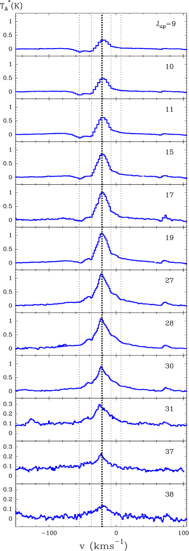
Figure 2: HC₃N pure rotational lines toward the proto-planetary nebula CRL618 in the ground vibrational state. The thick dotted line marks the LSR velocity of the source. The thin dotted lines mark interesting features in the line profile discussed in the text.

The profiles of HC₃N rotational lines within the ground vibrational state (see figure 2) show evidence of the high velocity molecular wind (HVMW), also seen in lines of CO and other molecules. In HC₃N, the HVMW component of the line profile extends some 200 kms^-1 in some cases (see figure 3). In addition to this one, there is another component associated to a slowly expanding molecular envelope around the ultracompact HII region. This component has a maximum half power width of about 18 kms^-1 and is approximately centered at the LSR velocity of CRL618 (-21.3 kms^-1). Two different absorption dips are present (see figure 2). The first one appears at -37 kms^-1 in all the lines at least up to J=37–36. It turns out that this feature is related to the [ 1 0 0]E component of the rotational transitions of the (0100) state. The other absorption feature at -55 kms^-1 is due to expanding gas in the line of sight of the continuum source and is also found in low-J HCN (Neri et al. 1992) and CO (Cernicharo et al. 1989, Herpin et al. 2002). On the red side of the line, between approximately -8 and 7 kms^-1, there is evidence of emission that Neri et al. 1992 attributed to an unresolved structure located to the North-East of the HII region.

4.3 Vibrationally excited HC₃N

4.3.1 The (0001) vibrational state

The HC₃N rotational lines in the (0001) vibrational level, at least below J_up $\sim$ 20, still trace gas at higher velocities than that seen in rotational lines corresponding to higher energy vibrational levels (see below). For example, the J=15-14 transition in (0001) shows an absorption dip that clearly starts below -50 kms^-1, more than 30 kms^-1 apart from the LSR velocity of the source (see figure 3). However, for J_up above 20 this colder and faster outflow is not significant in the level population anymore.

4.3.2 Other vibrational states

The HC₃N lines in the rest of the detected vibrationally excited states display patterns with many common characteristics. The lines appear dominantly in emission at 1.3 mm (at the IRAM-30m radiotelescope) and at shorter wavelengths (CSO observations at 0.850 mm) with a half power width ranging from 5 to 16 kms^-1, but mostly around 8-10 kms^-1. However, the majority of lines in the 2 and 3 mm windows show P-Cygni profiles, with the absorption part being systematically deeper at lower frequencies. This absorption is centered in the range -26 to -31 kms^-1, as expected for an expanding envelope with velocities around 5-10 kms^-1 surrounding the central continuum source at the LSR velocity of CRL618. The absorption is less deep and shifts to more negative velocities as the emission part gets stronger with increasing J. At frequencies well below 80 GHz, almost all lines, from other species also, appear strictly in absorption. The velocity of the absorption feature in HC₃N rotational lines, with J_up $<$ 7, in different vibrationally excited states, observed with the Effelsberg 100m radiotelescope (Wyrowski et al. 2003) is around -26 or -27 kms^-1. Thorwirth et al. 2003 also report HCN $\Delta$J=0, $\ell$-doubling transitions purely in absorption at the same velocity, as do Martín-Pintado et al. (1995) for NH₃ (3,3). The lowest transitions we have observed (J=9-8, J=10-9) in some highly excited vibrational states such as (0100) and (1000) do not show emission and the absorption feature is also centered around -27.5 kms^-1.

5 Discussion

In this work we assume that the bulk of vibrationally excited HC₃N emission comes from a compact envelope expanding at about 10 kms^-1 around the central continuum source. The availability of rotational ladders in so many different vibrationally excited HC₃N states should provide a quite precise picture of the size ratio of the slowly expanding gas region with respect to the continuum source, the shape of the envelope, the temperature profile, velocity field and HC₃N density distribution. All this is explored in sections 5.1 and 5.2.

5.1 Model

In order to reproduce the observed rotational HC₃N ladders we have built a model, for LTE conditions, of an expanding envelope around a continuum source. Because of blending with the selected HC₃N lines for the analysis, we have also introduced HC₅N with an abundance ratio of 1/3 respect to HC₃N (Cernicharo et al. 1987; Guélin and Cernicharo 1991), and isotopic species of HC₃N using a ¹²C/¹³C ratio of 15.

The lines are formed as follows: First, the central continuum source is responsible for the observed continuum level. The gas situated between the continuum source and the Earth absorbs that continuum and also emits. The gas in regions outside the line of sight to the continuum source contributes by emission only. The continuum source is considered opaque to the emission of the gas behind it. The spectrum of the continuum source and its size ratio with respect to the gas region, turn out to be key parameters to fit the simulations to the observed HC₃N rotational lines. The absorption takes place primarily at the terminal velocity of the expanding envelope in front of the continuum source. The emission can help to “fill” the absorption dip depending on the characteristics of the velocity field and the turbulence velocity.

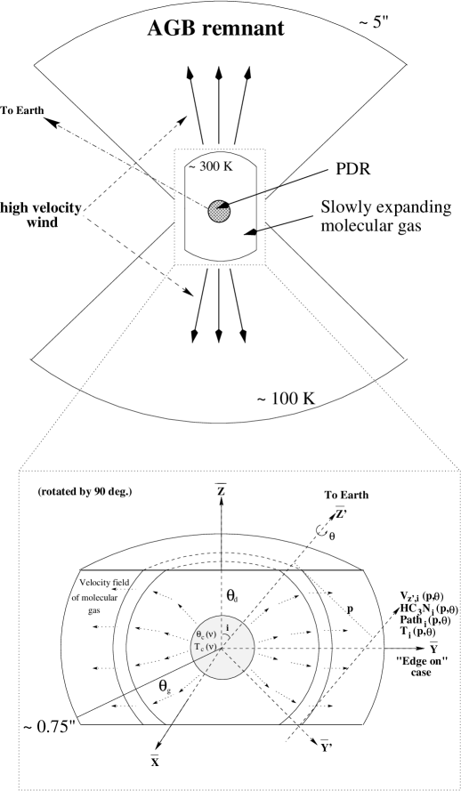
Figure 4: Model of CRL618 including the description of the expanding elongated structure considered to account for the observed HC₃N line profiles. See text for details about the different parameters of the model.

The simplest model considers a spherical expanding envelope of gas surrounding a central continuum source (also spherical). The envelope is divided into different shells where the total HC₃N number density and the temperature vary according to a power law, and radial expansion and turbulent velocities are linearly interpolated between input values at the boundaries. Such a simple model can only approximately reproduce the main observational characteristics of the HC₃N rotational ladders in CRL618. A more complex model has been developed to account for an elongated envelope with non-radial velocity components. We consider an external angular size of the (spherical) slowly expanding envelope $\theta_{g}$ and then we truncate it so that, in the truncation direction, the size is: $\theta_{d}$=$\theta_{g}\times r_{d}$, $r_{d}$ being the truncation parameter (see figure 4). Other geometric details of this model are the following: A first coordinate system (XYZ) is defined with the Z axis running in the direction where the sphere is truncated, and X, Y are orthogonal to each other and to Z. The velocity field will be a function of [(x²+y²)${}^{\frac{1}{2}}$,z] (azimuthal symmetry in the XY plane), and the temperature and gas densities will only be a function of r=(x²+y²+z²)${}^{\frac{1}{2}}$ (radial symmetry). The second coordinate system has the axis X’ in common with X just described, and the remaining two (Y’,Z’) are rotated respect to (Y,Z) by an angle $i$ so that Z’ points to the Earth (line of sight). The “edge-on” case therefore corresponds to i=90^o. The continuum source is spherical with an angular radius $\theta_{c}$. The value of $\theta_{c}$ has to be in the range 0.15”-0.4” in order to be compatible with data presented in section 4.1. We use as input parameter its ratio $r_{c}$ respect to the external angular size of the slowly expanding envelope, $r_{c}$=$\theta_{c}$/$\theta_{g}$. The effective temperature of the continuum source would depend on that size in order to match the observed continuum. In general, the equivalent size $\theta_{c}$ would be a function of frequency. However, a constant size and a frequency dependent $T_{c}$, characterized by a spectral index $s$ (see following equation), fit the data very nicely (see figure 1 and table 2).

$$T_{cont}(\nu)=T_{cont}({\rm 200\;\;\;GHz})[\nu/200]^{s}{\rm,}$$ (1)

In the elongated envelope case, the velocity field cannot be exactly radial: $\vec{v}=v_{r}\vec{r}+v_{xy}\vec{r_{xy}}$ ($v_{xy}\neq 0$ if r${}_{d}<$1). The extra velocity component in the XY plane makes the velocity pattern look as in figure 4. This kind of velocity field has the advantage of having gas with the same velocity projection in regions in and out the column between the continuum source and the Earth. Some extra gas is thus allowed to contribute filling the absorption dip (not only the turbulence velocity helps to do this, see figure 5). The velocity field remains unchanged by rotation respect to the Y or Z axis. Therefore, in the $i$=0^o,90^o cases (“edge-on” or “orthogonal” envelope cases), only the radiative transfer results as a function of the impact parameter $p$ (defined as an angle) have to be used in the numerical convolution with the antenna beam pattern. If $i$ takes any intermediate value, the numerical integration becomes dramatically more time consuming (10-100 times) because the azimuthal symmetry respect to the XY’ plane is broken and the convolution has to be performed in both $p$ and $\theta_{XY^{\prime}}$ (azimuthal angle around the Z’ or line-of-sight axis, see figure 4).

As we have seen, the model has an important number of parameters. Some of them can be fixed with some confidence, based on data such as the continuum flux (see figure 1) and the estimated distance to the source. The other parameters, velocity field, kinetic temperature, shape of the slowly expanding envelope, ratio between its size and that of the continuum source, and HC₃N column density, can be constrained by running a number of models. It is quite straightforward to find the best values for all parameters, with the exception of the kinetic temperature and HC₃N column density. This is discussed below.

5.2 Constraining the physical parameters

The first step in the simulation process has concentrated on the continuum source. We have considered different sizes for it (constant with frequency) and we have calculated its effective temperature at a reference frequency (200 GHz) and the spectral index, $s$, to match the observed continuum (figure 1). Based on the references given in section 4.1, the range of sizes we have explored is 0.15” to 0.40”. The results are given in table 2. For each set of values, the fit to our continuum data is very good, typically as shown on figure 1. As the external size of the gas region we are modeling is around 1.5” and the ratio of this size to the continuum source size is a key parameter for reproducing the observed line profiles, the preferred values among the five given alternatives are highlighted in bold face.

As the number of physical parameters and lines observed are both large, a general numerical fit to constrain all physical parameters simultaneously is not possible. Rather, it is necessary to run a large number of models in several steps in order to find a reasonable match to all the observed HC₃N rotational ladders. As this is very time consuming, the simulations have been restricted to the (0002), (0010), (0100), (0003), (0011), (1000), (0012), and (0102) vibrational states, as explained in section 4.

In the search for the best solution we also need to define a parameter to evaluate the quality of the fit. Ideally, this parameter has to give equal weight to the different lines, independently of the frequency resolution. We thus defined an overall $\chi$ as follows:

$$\chi=\frac{1}{N_{l}}\sum_{i}\sqrt{\frac{\sum_{j}|Yd-Ym|^{2}}{N_{ch}}}$$ (2)

where $N_{l}$ is the number of suitable lines in figure 6, $Yd(j)$ are the data (total flux divided by the contiuum flux), $Ym(j)$ are the model results, $N_{ch}$ is the number of channels where $Ym(j)\neq 1.0$, i.e. we do not consider channels where the signal is just the continuum level, or lines from species other that HC₃N or HC₅N. In addition, if a line from other chemical species overlaps with those from HC₃N or HC₅N, the corresponding spectrum is discarded. Note also that in figure 6 not all the $\ell$-type lines are shown in each case due to the sometimes large velocity separation. Only the data shown in the figure are used to calculate $\chi$. Blending between different vibrational states or within the same vibrational state has been treated in our simulations.

The two parameters that we have tried to determine by looking at $\chi$ in a grid of models are the temperature of the gas and the HC₃N column density. In order to illustrate how the best solution (6) is found we show in figure 7 the values of parameter $\chi$ as a function of these two parameters. The overall set of parameters characterizing the slowly expanding molecular envelope is then shown on table 3.

The kinetic temperature found here (250-275 K) is in very good agreement with the value derived from ISO IR data by Cernicharo et al. 2001a,b. The average column density of absorbing HC₃N in front of the continuum source is found to be in the range 2.0-3.5$\cdot$10¹⁷ cm^-2. HC₃N column densities in front of the continuum source where determined to be 5$\cdot$10¹⁶ cm^-2 by Cernicharo et al. (2001a) from ISO observations of HC₃N (0100) and (0001) bending modes in absorption around 14 $\mu$m. The difference between both estimates could be related to two facts: First, the ISO data lacks the spectral resolution needed to fully resolve the individual lines used for the estimate. Second, Cernicharo et al. 2001a assumed the same filling factor for the continuum source and the absorbing gas. However, dust emission at the wavelength of the (0100) mode of HC₃N, and in particular at that of the (0001) mode could contribute from a region larger than the zone where HC₃N is produced. The IR ISO data could give the same HC₃N column density as that derived here from the millimeter lines, if the continuum level to be considered for the former calculation (originated from behind the gas) is only about 30-50 % of the total observed continuum flux at 14 $\mu$m.

6 Conclusions

In this paper we have shown that toward the protoplanetary nebula CRL 618:

• HC₃N is detected in its ground and other vibrational states with energies up to 1100 cm^-1. The J_up range surveyed is from 9 to 30 (IRAM 30m telescope, 15 vibrational states detected) and 31 to 39 (CSO telescope, detections in 5, possibly 6 vibrational states). The observed frequencies match very well those provided by the model of Fayt et al. (2004).

• The line profiles of the HC₃N ground vibrational state show evidence of the HVMW already found in the strong lines of CO, HCN and HCO⁺ with the same velocity span ($\sim$200 kms^-1). Other vibrational states do not show this component in their rotational lines, except for the (0001) state that shows it marginally in the lowest J lines. Absorption features in the rotational lines of the ground vibrational state appear at similar velocities to those of features already seen in CO and HCN. The only exception is the one centered at $\sim$-37 kms^-1 that is due to blending with (0100)[1 0 0]E lines.

• The pure rotational transitions in vibrationally excited states of HC₃N show an evolution in their line profiles with increasing J going from almost pure absorption centered at around -27 or -28 kms^-1, to P-Cygni profiles and, finally pure emission centered quite close to the LSR velocity of the source. The intermediate-J P-Cygni profiles have the emission part also centered quite close to the LSR velocity, while the minimum of the absorption part shifts to more negative velocities and becomes less deep as J increases. The exact value of J_up at which the absorption disappears changes only slightly with the vibrational state: It happens at slightly higher values as the energy of the vibrational state increases. For example, no absorption is observed in the J=24-23 transition of the (0001) vibrational state, whereas some absorption is still seen in the J=26-25 line of the (1000) one. Some rotational lines within the (0001) state still trace larger velocities than those in the other vibrationally excited states.

• An model for the slowly expanding envelope, under LTE, built to explore the physical parameters that explain the extensive set of HC₃N rotational lines detected ($\sim$300, although the fit has been done to a subset of 116) has shown that:

  1. The size of the inner continuum source is $\sim$0.27” with an effective temperature of $\sim$3900 K at 200 GHz and a spectral index of -1.12.

  2. The external size of this slowly expanding envelope is $\sim$ $\theta$=1.5”.

  3. The expansion velocity field has a radial component ranging from 5 to 12 kms^-1 with a possible extra azimuthal component reaching 6 kms^-1 at $\theta$=1.5”.

  4. The turbulence velocity is $\sim$3.5 kms^-1.

  5. The temperature of the envelope is in the range 250-275 K.

  6. The HC₃N column density in front of the continuum source is in the range 2.0-3.5$\cdot$10¹⁷ cm^-2 (the best fit is obtained for 2.8$\cdot$10¹⁷ cm^-2).

Table 1: Observed line parameters of the J=12-11 and J=26-25 transitions in all vibrationally excited states of HC₃N (see text for notation) detected toward CRL618 (v_1,2: position in kms^-1, $\Delta$v_1,2 width in kms^-1, A_1,2 area in K$\cdot$km^-1; 1 refers to the emission part and 2 to the absorption part of the line profile). In addition to the vibrational states show here, the (0111) at more than 1200 cm^-1 is tentatively detected.

V. state	type of	J=12-11							J=26-25
[E cm-1]	$\ell$ transition	$\nu$ (GHz)	v1	$\Delta$v1	A1	v2	$\Delta$v2	A2	v1	$\nu$ (GHz)	$\Delta$v1	A1	v2	$\Delta$v2	A2
(0001)	[ 0 0 1]F	109.598825	-20.9	14.9	3.6	-31.6	22.3	-3.3	237.432241	-20.8	18.7	7.2
[223]	[ 0 0 1]E	109.442011	blended with (0010)[ 0 1 0]F						237.093375
(0002)	[ 0 0 0]E	109.865960	blended with [ 0 0 2]E,F						237.968847	-23.7	16.0	5.9
[426]	[ 0 0 2]E	109.870288	blended with [002]F,[000]E						238.053887	-21.6	11.3	3.5
	[ 0 0 2]F	109.865960	blended with [002]E,[000]F						238.010133	-21.5	10.6	3.2
(0010)	[ 0 1 0]E	109.352748	-21.3	7.4	0.47	-29.8	7.3	-0.90	236.900342
[499]	[ 0 1 0]F	109.438718	blended with (0010)[ 0 1 0]F						237.086494
(0100)	[ 1 0 0]E	109.183008	blended with ground state of HC3N						236.529566	blended with ground state of HC3N
[663]	[ 1 0 0]F	109.244206	-21.3	11.0	0.35	-28.4	6.6	-0.66	236.661402	-20.5	8.4	0.44
(0003)	[ 0 0 1]E	110.050809	-21.3	9.0	0.37	-28.7	6.9	-0.59	238.401147	-21.2	7.47	1.0
[669]	[003]E+F	110.211793	-21.3	4.1	0.02	-29.5	7.7	-0.79	238.771331	-21.3	12.0	1.8	-31.1	5.8	-0.3
	[ 0 0 1]F	110.366468	-21.3	14.6	0.7	-28.3	6.2	-0.62	239.082313	-20.9	11.5	1.4
(0011)	[ 0 1-1]E	109.736687	$\sim$3 MHz away from [ 0 1-1]F						237.681318	-22.1	9.2	1.5	-28.2	14.2	-0.7
[721]	[ 0 1-1]F	109.740137	$\sim$3 MHz away from [ 0 1-1]E						237.713612	blended with (0101)[ 1 0 1]F
	[ 0 1 1]F	109.749784	$\sim$3 MHz away from [ 0 1 1]E						237.783921	-21.8	9.9	1.9	-26.9	15.5	-1.0
	[ 0 1 1]E	109.752621	$\sim$3 MHz away from [ 0 1 1]F						237.814870	-22.9	8.6	1.4	-28.3	11.0	-0.7
(1000)	[ 0 0 0]E	109.023292	-21.3	12.7	0.22	-27.9	6.2	-0.40	236.184052	-23.6	8.8	0.35	-27.8	4.1	-0.22
[880]
(0101)	[ 1 0-1]F	109.558099	-21.3	6.0	0.07	-28.0	4.5	-0.25	237.336037	-21.3	12.0	0.73	-29.0	5.2	-0.30
[886]	[ 1 0-1]E	109.549318	-21.3	7.5	0.16	-27.5	3.9	-0.18	237.409821	blended with (0001)[ 0 0 1]F
	[ 1 0 1]F	109.564687	-21.3	7.5	0.16	-27.5	5.5	-0.29	237.716883	blended with (0011)[ 0 1-1]F
	[ 1 0 1]E	109.553091				-27.5	3.9	-0.18	237.898318	-19.8	11.4	1.04

Table 1: Continued.

V. state	type of	J=12-11							J=26-25
[E cm-1]	$\ell$ transition	$\nu$ (GHz)	v1	$\Delta$v1	A1	v2	$\Delta$v2	A2	v1	$\nu$ (GHz)	$\Delta$v1	A1	v2	$\Delta$v2	A2
(0004)	[ 0 0 0]E	110.543693	-21.3	10.9	0.2	-27.4	5.2	-0.35	239.370230	-21.1	8.8	0.63
[892]	[ 0 0 2]F	110.548972							239.125296
	[004]E+F	110.554367	-21.3	7.1	8.9	-28.6	4.8	-0.23	239.510881
	[ 0 0 2]E	110.562578	-19.9	10.5	0.6				238.962431
(0012)	[ 0 1 0]E	109.989997				-27.4	5.2	-0.30	238.254341	-21.7	8.1	0.53
[944]	[ 0-1 2]F	110.035645				-28.2	4.5	-0.18	238.388217	-20.2	9.3	0.64
	[ 0 1 2]E+F	110.097528	-21.3	5.7	0.09	-27.8	5.6	-0.34	238526.950	-22.5	8.5	0.58	-31.2	6.1	-0.28
	[ 0-1 2]E	110.148765	-21.3	5.0	0.06	-27.7	4.7	-0.16	238.631641	-21.5	8.8	0.79
	[ 0 1 0]F	110.189752				-27.2	5.0	-0.18		-21.2	9.5	0.75
(0020)	[ 0 0 0]E	109.522442				-27.4	4.3	-0.17	237.270155
[998]	[ 0 2 0]E	109.616120	-21.3	7.5	0.23	-29.4	7.7	-0.38	237.468947	-21.3	8.2	0.77		e
	[ 0 2 0]F	109.616295	-21.3	7.2	0.24	-28.8	8.3	-0.41	23.7470747	-19.1	7.5	0.73
(1001)	[ 0 0 1]E	109.306687				-27.0	6.0	-0.17	236.795297	-20.0	4.5	0.10	-28.5	4.4	-0.12
[1103]	[ 0 0 1]F	109.469407				-27.0	6.0	-0.12	237.145656	-21.3	9.5	0.27
(0102)	[-1 0 2]E	109.789853	blended with C18O						237.803492	-19.9	5.3	0.25
[1109]	[ 1 0 0]F	109.847627							237.956672	blended with (0002)[ 0 0 0]E
	[ 1 0 2]E	109.905021							238.164654	-20.3	5.6	0.22
	[ 1 0 2]F	109.868821							237.995859	blended with (0002)[ 0 0 2]F
	[ 1 0 0]E	109.953634							238.178301	-21.8	8.6	0.39
	[-1 0 2]F	109.989048							238.318310
(0005)	[ 0 0 1]E	110.655045	-21.3	11.7	0.1	-28.2	4.8	-0.13	230.471871	-21.3	7.9	0.23	-28.5	4.6	-0.14
[1115]	[ 0 0 1]F	111.131162	-21.3	15.6	0.26	-27.5	2.8	-0.07	231.456018
	[ 0 0 5]E+F	110.895474				-28.2	4.8	-0.13	231.009985
	[ 0 0 3]E+F	110.902009	-21.3	2.7	0.02	-28.2	5.0	-0.13	231.031080

Table 2: Set of models to describe the central continuum source of CRL618 according to the parameters defined in equation 1. The preferred is in bold face (see figure 1).

size (“)	Tcont(200 GHz)	spectral index $s$
0.18	8600	-1.15
0.22	6400	-1.15
0.27	3900	-1.12
0.32	3200	-1.12
0.36	2300	-1.12

Table 3: Model parameters of expanding envelope that provide the best fit to the data shown in figure 6.

parameter	value	units
$\theta_{g}$	1.5	arcsec
rd	0.7	-
$i$	90	degrees
$T_{gas}$ (at $\theta$=$\theta_{c}$)	263	K
$T_{gas}$ (at $\theta$=$\theta_{g}$)	263	K
$v_{r}$ (at $\theta$=$\theta_{c}$)	5.0	kms-1
$v_{r}$ (at $\theta$=$\theta_{g}$)	12.0	kms-1
$v_{xy}$ (at $\theta$=$\theta_{c}$)	0.0	kms-1
$v_{xy}$ (at $\theta$=$\theta_{g}$)	6.0	kms-1
$v_{turb}$ (at $\theta$=$\theta_{c}$)	3.5	kms-1
$v_{turb}$ (at $\theta$=$\theta_{g}$)	3.5	kms-1
$[$HC3N$]$ (at $\theta$=$\theta_{c}$)	154	cm-3
$d$	-1.8	-
HC3N col. density	2.0-3.5$\cdot$1017	cm-2
at $p$$<$rc

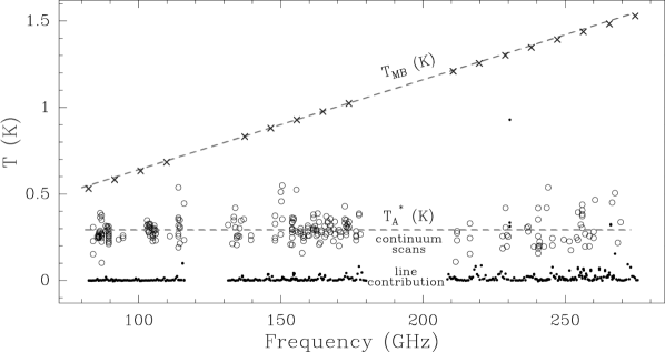
Figure 1: Open circles: Millimeter-wave continuum of CRL618 observed by the IRAM 30m telescope (T${}_{A}^{*}$ scale, from pointing observations on CRL618 in continuum mode). Horizontal dashed line: Fit of these data to a horizontal line. Inclined dashed line: Fit translated into T_MB. Crosses: Simulated continuum T_MB by our model (see sections 5.1 and 5.2).

Figure 3: Velocity components of HC₃N lines toward CRL618. In the ground vibrational state (top two spectra) we see broad wings associated to the HVMW discovered by Cernicharo et al. 1989 and a narrower emission due to the slowly expanding gas envelope around the HII region. A blending with HC₃N (0100) causes the absorption feature at $\sim$-37 kms^-1. The absorption centered at -55 kms^-1 is also seen in other abundant molecules such as HCN and CO. In vibrationally excited states (bottom two spectra) the HVMW component is not visible. At low-J the absorption of the slowly expanding gas in front of the continuum source is seen centered at $\sim$-27 kms^-1. However, the absorption dissapears at J $>$ 20 for the particular case of the (0001) state (the J number where this happens slightly depends on the vibrational state). Still, rotational lines within the (0001) state trace larger velocities than those in higher vibrational states, although it is not the HVMW.

Figure 5: Fit of observed HC₃N rotational line toward CRL618 and separate contribution from gas in and out of the line of sight to the continuum source. The physical parameters correspond to those listed in table 3.

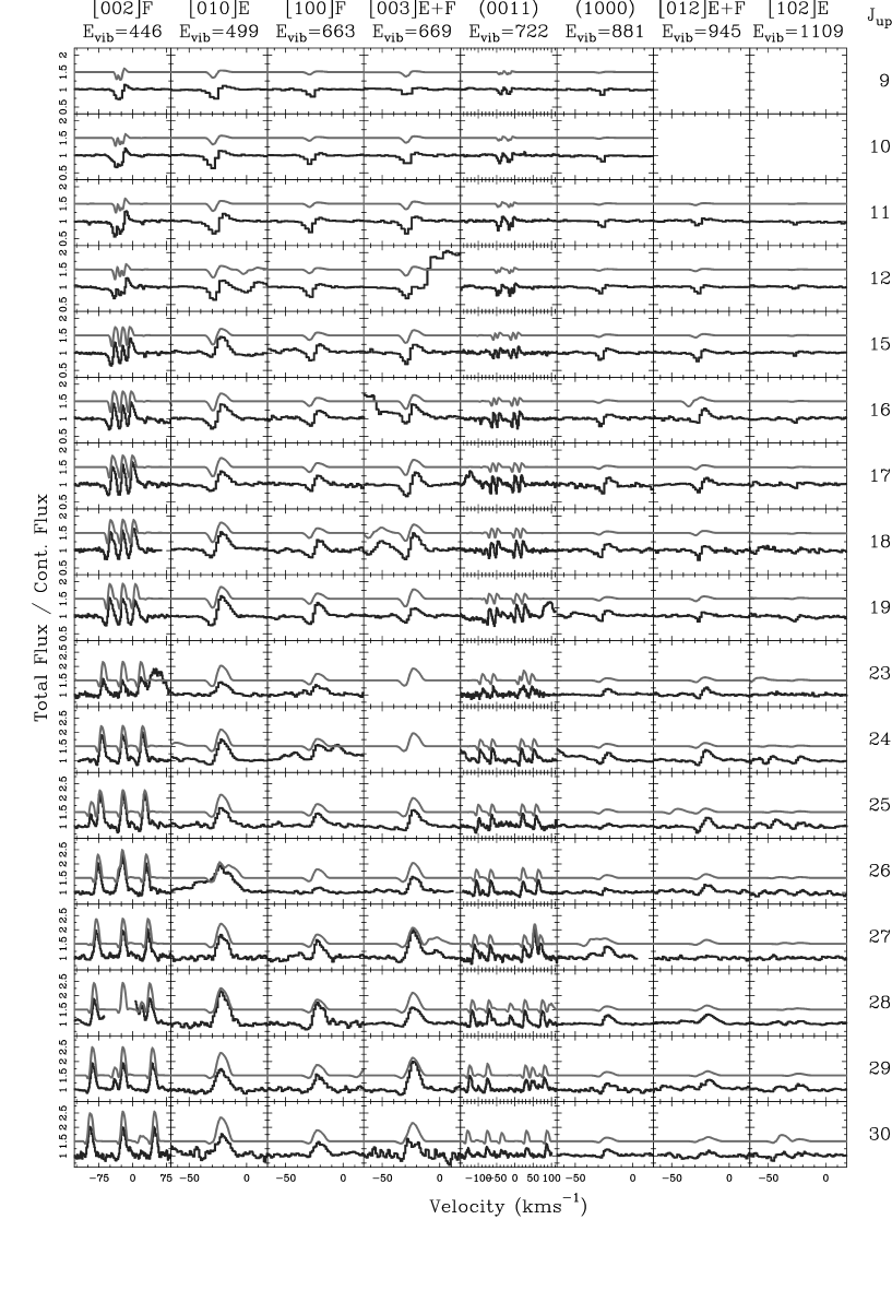
Figure 6: Observed HC₃N pure rotational lines toward the proto-planetary nebula CRL618 in several vibrationally excited states from 446 to 1109 cm^-1 compared to the results of our model. In a few cases the observation is not shown because the corresponding HC₃N line is totally masked by a stronger line from another molecule.

Figure 7: Value of $\chi$ (defined in equation 2) for the grid of models run to find the temperature of the CRL618 slowly expanding envelope and the HC₃N column density that best fits the data shown on figure 6.

References

- (1) Bell, M. B., Feldman, P. A., Travers, M. J., McCarthy, M. C., Gottlieb, C. A., & Thadeus, P. 1997, ApJ, 483, L61.
- (2) Bujarrabal, V., Gómez-González, J., Bachiller, R., & Martín-Pintado, J. 1988, A.&A., 204, 242
- Cernicharo et al. (1987) Cernicharo J., Guélin M., Menten K.M. and Walmsley C.M. 1987, A&A, 181, L1
- (4) Cernicharo, J. Guélin, M., Martin-Pintado, J., Peñalver, J., & Mauersberger, M. 1989, A&A, 222, L1
- (5) Cernicharo, J., Heras, A. M., Tielens, A.G.G.M., Pardo, J. R., Herpin, F., Guélin, M., Waters, L.B.F.M. 2001a, Ap.J. 546, L123.
- (6) Cernicharo, J., Heras, A. M., Pardo, J. R., Tielens, A. G. G. M., Guélin, M., Dartois, E., Neri, R. & Waters, L. B. F. M. 2001b, Ap. J., 546, L127.
- (7) Cernicharo, J., 2004, Ap.J., 608, L41.
- (8) Cox, P., Huggins, P. J.; Maillard, J.-P.; Muthu, C.; Bachiller, R.; Forveille, T.; 2003, Ap. J. 586, L87.
- (9) Fayt, A., Vigouroux, C., Willeart, F., Margules, L., Constantin, L.F., Demaison, J., Pawelke, G., Mkadmi, El B., Bürger, H., J. Mo. Struct., 2004, in press.
- Guélin and Cernicharo (1991) Guélin M., Cernicharo J. 1991, A&A, 244, L21
- (11) Herpin, F., Goicoechea, J.R., Pardo, J.R., Cernicharo, J. 2002, Ap.J., 577, 961
- (12) Kwok, S. & Feldman, P.A. 1981, Ap.J., 267, L67
- (13) Kwok, S. & Bignell, R.C. 1984, Ap.J., 276, 544
- (14) Martín-Pintado J., Gaume R., Bachiller R. Johnston K. 1993, Ap.J., 419, 725
- (15) Mbosei, L., Fayt, A., Dréan, P., & Cosléou, J. 2000, J. Mol. Structure, 517-518, 271.
- (16) Neri, R., Garcia-Burillo, S., Guélin, M., Cernicharo, J., Guilloteau, S. & Lucas, R. 1992, A.&A., 262, 544
- (17) Sánchez-Contreras, C., & Sahai, R., 2004, Ap.J., 602, 960.
- (18) Shibata, K. M., Deguchi, S., Hirano, N., Kameya, O., Tamura, S. 1993 Ap.J., 415, 708.
- (19) Spergel, D. N., Giuliani, J.L. Jr., Knapp, G.R. 1983 Ap.J., 275, 330.
- (20) Thorwirth, S., Wyrowski, F., Schilke, P., Menten, K. M., Brünken, S., Müller, H. S. P., and Winnewisser, G., Ap. J., 586, 338-343, 2003
- (21) Walmsley, M., Chini, R., Kreysa, E., Steppe, H., Omont, A. 1991, A.&A., 248, 555
- (22) Wyrowski, F., Schilke, P., & Walmsley, C. M. 1999, A.&A., 341, 882
- (23) Wyrowski, F., Schilke, P., Thorwirth, S., Menten, K. M., and Winnewisser, G., Ap. J., 586, 344-355, 2003.