Multi-band optical micro-variability observations of the BL Lac object S4 0954+658

We have observed S4 0954+658 in the $B,V,R$ and $I$ bands for one night in March and two nights in April, 2001, and in the $B$ and $I$ bands for four nights in May, 2002. The observations resulted in almost evenly sampled light curves, $3-8$ hours long, with an average sampling interval of $\sim 5-15$ min. Because of the dense sampling and the availability of light curves in more than one optical bands we are able to study the intra-night flux and spectral variability of the source in detail. Significant observations were observed in all but one cases. On average, the flux variability amplitude, on time scales of minutes/hours, increases from $\sim 2-3\%$ in the $I$, to $\sim 3.5-5.5\%$ in the $B$ band light curves. We do not detect any flares within the individual light curves. However, there is a possibility that the April 2001 and late May 2002 observations sample two flares which lasted longer than $\sim 1-3$ days. The evidence is only suggestive though, due to the limited length of the present light curves with regard to the duration of the assumed flares. No spectral variations are detected during the April 2001 observations. The source flux rises and decays with the same rate, in all bands. This variability behaviour is typical of S4 0954+658, and is attributed to geometrical effects. However, significant spectral variations are observed in May 2002. We find that the spectrum hardens/softens as the flux increases/decreases, respectively. Furthermore, the “hardening” rate of the energy spectrum is faster than the rate with which the spectrum becomes “redder” as the flux decays. We also find evidence (although of low statistical significance) that the $I$ band variations are delayed with respect to the $B$ band variations. If the May 2002 observations sample a flaring event, these results suggest that the variations are caused by energetic processes which are associated with the particle cooling and the source light travel time scales.

1 Introduction

BL Lac objects are one of the most peculiar classes of active galactic nuclei (AGN). They show high polarization (up to a few percent, as opposed to less than $\sim 1\%$ for most AGNs) and usually do not exhibit strong emission or absorption lines in their spectra. They also show continuum variability at all wavelengths at which they have been observed, from X-rays to radio. In the optical band they show large amplitude, short time scale variations. The overall spectral energy distribution of BL Lacs shows two distinct components in the $\nu-\nu F_{\nu}$ representation. The first one peaks from mm to the X–rays, while the second component peaks at GeV–TeV energies (e.g. Sambruna et al. 1996). The commonly accepted scenario assumes that the non-thermal emission from BL Lacs is synchrotron and inverse-Compton radiation produced by relativistic electrons in a jet oriented close to the line of sight.

S4 0954+658 is a well studied BL Lac object in the optical bands. Its optical variability has been studied by Wagner et al. (1990, 1993). Wagner et al. (1990) found large amplitude variations (of the order of $\sim 100\%$) on time scales as short as 1 day. Wagner et al. (1993), using a well sampled, 1 month long $R$ band light curve, observed symmetric flares, with a max–to–min variability amplitude of the order of $\sim 4-5$. Raiteri et al. (1999) presented a comprehensive study of the optical (and radio) band variability of the source using $4$ year long optical light curves. They also detected large amplitude, fast variations. Studying the $B-R$ colour variations, they also found that the mid and long-term variations in the source are not associated with spectral variations.

In this work, we present simultaneous $B$, $V$, $R$ and $I$ band monitoring observations of S4 0954+658, which were obtained in the years 2001 and 2002 from Skinakas Observatory, Crete, Greece. The quality of the light curves is similar to those presented by Papadakis et al. (2003) in the case of BL Lac itself. Compared to previous observations, the biggest advantage of the present observations is that they resulted in light curves at different energy bands, with a dense, almost evenly sampling pattern.

Our main aim is to use these light curves in order to investigate the flux and spectral variations of the source on time scales as short as a few minutes/hours. We find that, apart from variations which are best explained as being the product of geometric variations (in agreement with the past observations), the source also exhibits fast variations which are most probably caused by changes in the energy distribution of the high energy particles in the synchrotron emitting source.

2 Observations and data reduction

S4 0954+658 was observed for 3 nights in 2001 and 4 nights in 2002 with the 1.3 m, f/7.7 Ritchey-Cretien telescope at Skinakas Observatory in Crete, Greece. The observations were carried out through the standard Johnson $B,V$ and Cousins $R,I$ filters. The CCD used was a $1024\times 1024$ SITe chip with a 24 $\mu$m² pixel size (corresponding to $0^{\prime\prime}.5$ on the sky). The exposure time was 300, 240, 120 and 120 s for the $B,V,R$ and $I$ filters, respectively. In Table 1 we list the observation dates, and the number of frames that we obtained each night. During the observations, the seeing varied between $\sim 1^{\prime\prime}-2^{\prime\prime}$. Standard image processing (bias subtraction and flat fielding using twilight-sky exposures) was applied to all frames.

Table 1: Date of observations, and number of frames (nof) obtained at each optical band.

Date	$B$	$V$	$R$	$I$
	(nof)	(nof)	(nof)	(nof)
26/03/01	–	–	24	24
18/04/01	16	16	17	16
19/04/01	5	5	5	5
23/05/02	27	–	–	27
28/05/02	19	–	–	19
29/05/02	24	–	–	24
20/05/02	24	–	–	24

We performed aperture photometry of S4 0954+658 and of the comparison stars 2, 3, 4, and 7 of Raiteri et al. (1999) by integrating counts within a circular aperture of radius $10^{\prime\prime}$ centered on the objects. The remaining 5 comparison stars in the list of Raiteri et al. are also visible in the field of view. However the scatter in their light curves was larger than the scatter in the light curves of the 4 comparison stars that we kept. For that reason we decided not to use them. The error on the S4 0954+658 magnitude measurements in each frame were estimated as follows. First, we estimated the standard deviation ($\sigma$) of the comparison stars light curves, in each band, during the 2001 and 2002 observations. We consider these values as representative of the uncertainty in the magnitude estimation of the comparison stars within each observing period. Then, for each frame, the error on the S4 0954+658 magnitude was computed using the standard “propagation of errors” formula of Bevington (1969), taking into account the photometry error of the source’s measurement and the $\sigma$ values of the comparison stars.

The calibrated magnitudes were corrected for reddening using the relationship $A_{V}=N_{H}/2.23\times 10^{21}$ (Ryter 1996), in order to estimate the $V$ band extinction ($A_{V}$, in magnitudes). We assumed the column density value of $N_{H}=9.0\times 10^{20}$ cm^-2, derived from X–ray measurements with ROSAT (Urry et al. 1996). This value implies $A_{V}=0.40$, which is almost identical to the respective value of Schlegel et al. (1998) as taken from NED. Using the $A_{\lambda}$ versus $\lambda$ relationship of Cardelli et al. (1989) we found the extinction (in magnitudes) in the $B,R,$ and $I$ filters: $A_{B}=0.53,A_{R}=0.30$, and $A_{I}=0.19$. Finally, we converted the dereddened magnitudes into flux, without applying any correction for the contribution of the host galaxy, as it cannot be resolved even in deep HST images (Scarpa et al. 2000).

3 The observed light curves

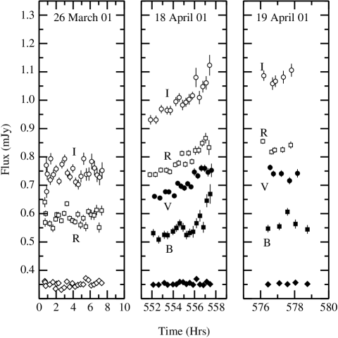
Figure 1: $B,V,R,$ and $I$ band light curves during the 2001 observations. Time is measured in hours from 19:00 UT on March 26, 2001. The small filled diamonds below the $B$ band light curve of S4 0954+658 show the $B$ band light curve of the comparison star 2 (open diamonds in the left panel show the $R$ band light curve of the same star). For clarity reasons, the standard star light curves are shifted to the same level of $\sim$ 0.35 mJy.

Figure 2: $B$ and $I$ band light curves during the 2002 observations. Time is measured in hours from 18:00 UT on May 23, 2002. As before with Figure 1, the small filled diamonds show the $B$ band light curve of the comparison star 2 (shifted to a mean of $\sim$ 0.033 mJy).

Figs. 1 and 2 show the dereddened $B,V,R,$ and $I$ light curves of S4 0954+658 during the 2001 and 2002 observations, respectively. In the same figures we also show the $B$ band light curve of the comparison star 2. While the light curve of this star (and of the other 3 comparison stars in all bands) does not show significant variations, intrinsic intra-night variations can be observed in most of the S4 0954+658 light curves. Use of the $\chi^{2}$ test shows that the hypothesis of a constant flux can be rejected at the $99.9\%$ significance level in all cases, except from the May 23, 2002 $B$ and $I$ light curves.

The source was at a brighter flux state in 2001. During the April 18 observations the source flux increases. In the same night, the $B$ band light curve shows a fast flux decrease (at around 557 hrs) which is absent in the $V,R,$ and $I$ light curves. However, when compared with the adjacent points, the flux decrease is significant at only the $\sim 2\sigma$ level. The April 19, 2001 light curves last for less than $\sim 3$ hours (due to bad weather we could not observe the source for a larger period). The $R$ and $I$ band light curves are quite similar, but the $V$ and $B$ band light curves look different. There is a hint that they may be anti-correlated, but no firm conclusions can be drawn due to the short duration of the observations. During the May 28, 2002 observations the source flux increases, while the opposite behaviour is observed in May 30, 2002. In fact, as Fig. 2 suggests, the late May 2002 light curves could be part of a “flare-like” event which lasted for more than $\sim$ 3 days. It is possible that the May 28, and the May 29-30 observations sample the flux increasing and decaying parts of the flare, respectively. No trends on time scales of $\sim$ hours are evident in the $R$ and $I$ band, March 26, 2001 light curves. However, as the $\chi^{2}$ test indicates, the small amplitude variations around the mean flux level are significant in this case. We find that $\chi^{2}=84.2$ and $60.8$ for the $R$ and $I$ band light curves, respectively. The number of degrees of freedom is 23. Consequently, the probability that we would observe these values by chance, if the flux remained constant during the observations, is less than $\sim 3\times 10^{-5}$, in both cases. Finally, the peak max–to–min variability amplitude is $\sim 15\%$ and $\sim 30\%$ during the April 2001, and May 2002 observations, respectively.

In order to compare the amplitude of the variations that we observe in the various light curves we computed their “fractional variability amplitude” ($f_{rms}$), as described in Papadakis et al. (2003). The average $f_{rms}$ of the 2000 $B$ and $I$ band light curves is $f_{rms,B}=3.2\pm 0.5\%$ and $f_{rms,I}=2.6\pm 0.3\%$, respectively (we have not considered the May 23 light curves, as they show no significant variations). The average $I$ band variability amplitude during the 2001 observations is $f_{rms,I}=2.8\pm 0.5\%$, consistent with the 2002 estimate. We also find that the average variability of the 2001 $R$ band light curves is $f_{rms,R}=4.0\pm 0.5\%$, while $f_{rms}\sim 5\%$ and $5.5\%$ for the April 18, 2001 $V$ and $B$ band light curves. We conclude that S4 0954+658 shows low amplitude variations ($\sim 2-5\%$ on average) on time scales of a few hours. Furthermore, the variability amplitude increases towards higher frequencies, i.e. from the $I$ to the $B$ band light curves.

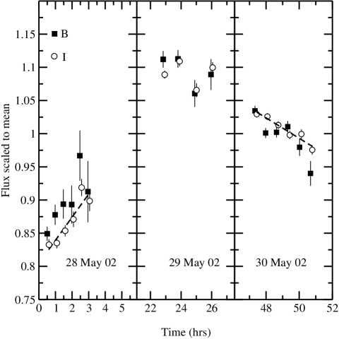
Figure 3: $B$ and $I$ band light curves in 2002 (filled squares and open circles, respectively) normalized to their average flux level. Time is measured in hours from the beginning (plus half an hour) of the May 28 $B$ band observations. In order to reduce the experimental noise, we have smoothed the May 28, 29 and 30 light curves using a bin size of 3, 6, and 4, respectively.

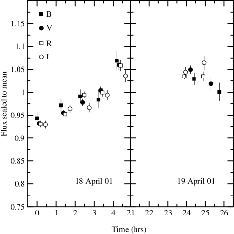
Figure 4: Same as Fig. 3 for the April, 2001 light curves (filled squares, filled circles, open squares, and open circles show the $B,V,R,$ and $I$ band light curves, respectively). The light curves have been smoothed out using a bin size of 3, except from the last point where a bin size of 2 was used. Time is measured in hours from the start of the April 18, $B$ band observations.

Figs. 3 and 4 show the late May 2002 and April 2001 light curves, normalized to their mean. In this way we can compare directly light curves in different energy bands, and investigate whether there are any differences in their variability pattern. On average, the $B$ over $I$ band flux ratio in May 28 appears to be larger than the same ratio of the May 29 and 30 observations. To investigate this issue further, we divided the $B$ and $I$ band normalized fluxes, within each night, and computed their weighted mean values, $<B/I>$. Our results are as follows: $<B/I>_{\rm May28}=1.04\pm 0.01,<B/I>_{\rm May29}=1.007\pm 0.008,$ and $<B/I>_{\rm May30}=0.992\pm 0.004$. They imply spectral variations, with the energy spectrum becoming progressively “redder” from the May 28 to the May 30 observations.

Furthermore, Fig. 3 shows clearly that the flux rises steeper than it decays, in both energy bands. In order to quantify this effect, we fitted the $I$ band light curves of the May 28 and 30 observations with a linear model of the form: $I_{norm}=a+\beta t$. The slope of this line, in units of “per cent/hrs”, is a measure of the normalized flux variation per unit time. The dashed lines in Fig. 3 show the best fitting models, which describe rather well the observed trends in the $I$ band light curves. The best fitting slopes are $\beta=3.5\%\pm 0.7\%$ and $-1.5\%\pm 0.2\%$ hrs^-1, for the May 28 and May 30 light curves, respectively. In other words, while the flux increases with a rate of $\sim 3.5\%$ per hour in May 28, it decreases with a slower rate (of $\sim 1.5\%$ per hour) in May 30. These differences suggest the presence of spectral variations during the May 2002 observations.

The situation is markedly different in April, 2001. First of all, the normalized flux rises with the same rate in all bands during the April 18 observation. Indeed, when we fit all the light curves with a linear model, the best fitting slope suggests a flux increase rate of $\sim 2.5\%$ per hour in all cases. The April 19 normalized light curves in Fig. 4 appear to be in agreement with each other. If we consider them together as a “single” light curve, and we fit them with the same linear model as above, we find that the flux decreases with a rate of $\sim 2\%$ per hour, similar to the flux increase rate of the previous night. Fig. 4 suggests that the April 18 and 19, 2001 light curves could be part of a single flare (like the late May 2002 observations) which lasted more than a day. This is only suggestive of course, due to the short duration of the observations (specially in April 19). However if it is true, our results imply that during the flare evolution, the flux rises and decays with the same rate, opposite to what we observe in May 2002.

4 Spectral variability

Using the dereddened light curves and the equation, $\alpha_{12}=\log(F_{1}/F_{2})/\log(\nu_{1}/\nu_{2})$, where $F_{1}$ and $F_{2}$ are the flux densities at frequencies $\nu_{1}$ and $\nu_{2}$, respectively, we calculated two-point spectral indices: $B-I$ for the 2001 and 2002 observations, and $V-I$, $R-I$ for the 2001 observations only. We have used consecutive observations, with a time difference less than $\sim 15$ min.

Fig. 5 shows the $\alpha_{BI}$ versus the $B+I$ normalized flux plot for the 2002 observations. We observe significant $\alpha_{BI}$ variations which are correlated with the source flux. During the May 28 observations the spectrum becomes progressively “bluer”/harder (i.e. $\alpha_{BI}$ increases) as the source brightens. We observe the same trend during the May 29 and 30 observations. As the source flux decreases, the spectrum becomes “redder”/softer. However, the spectral variations do not follow the same “path” in the [$(B+I)_{norm},\alpha_{BI}$] plane during the flux rise and decay phases. First of all, the average $\alpha_{BI}$ index in May 28 is larger than the average index during the May 29, and 30 observations. When the flux increases the spectrum is “bluer” than the spectrum during the flux decay, in agreement with our comments in the previous section regarding the normalized light curves in Fig. 3.

We used a simple linear model of the form $\alpha=A+B\times flux$ to describe quantitatively the relation between flux and spectral index. The dotted lines in Fig. 5 show the best fitting model to the May 28 and to the combined May29/30 data. The model describes the spectral variations well. The best fitting slopes are $1.0\pm 0.2$ and $0.5\pm 0.1$ for the spectral variations during the flux rise and decay phases, respectively. Their difference is $0.5\pm 0.2$. Although this is only a $2.5\sigma$ effect, it suggests that the spectral variability rate during the rise and decay phases of the light curves is different. The rate with which the spectrum hardens during the flux rise is faster than the rate with which the spectrum softens during the flux decay phase.

Finally, the arrows in Fig. 5 show the flux evolution during the late May 2002 observations. The source flux increases in May 28, and the spectrum becomes “bluer”. In the following two nights, the source flux decreases, and the spectrum becomes “redder”, but at smaller rate. If the late May 2002 observations are part of the same flaring event, Fig. 5 suggests that the variation of $\alpha_{BI}$ as a function of the normalized flux follows a loop-like path, in the clockwise direction, during the flux rising and decaying parts of the event.

Fig. 6 shows the $\alpha_{BI}$ and $\alpha_{VI}$ versus the respective normalized flux [i.e. $(B+I_{norm})$ and $(V+I_{norm})$, respectively] for the April 2001 observations. This figure shows clearly that there are no spectral variations during these observations. Comparison between the plots in Figs. 5 and 6 implies that the source varies in a different way during the 2001 and 2002 observations. This is in agreement with the result we reached in the previous section, when we compared the normalized 2001 and 2002 light curves. The fact that during the April 18 observations the spectral indexes $\alpha_{BI},\alpha_{VI}$, and $\alpha_{RI}$ (not shown in Fig. 6 for clarity reasons) remain constant is consistent with the result that the flux rise rate is the same at all energy bands. The spectral indices remained constant in the following night as well. If the April 18 and 19 observations are part of the same flare, the flux rise and decay rate are equal in all optical bands. We conclude that the April 18 2001 flare is symmetric, and evolves with no spectral variations.

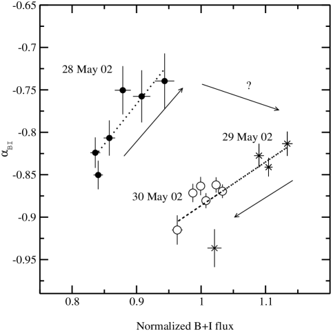
Figure 5: $B-I$ spectral index vs. the $B+I$ normalized flux for the 2002 observations. For clarity reasons, we have smoothed the data using the same bin size that we have used for the respective light curves in Fig. 3. The dotted lines show the best linear model fit to the data, while the arrows indicate the flux variability trend (i.e. flux increase or decrease) during the observations (see text for details).

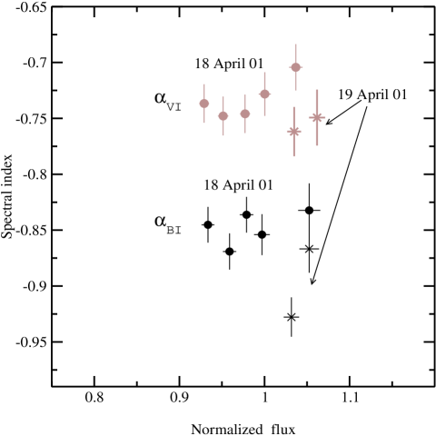
Figure 6: $B-I$ (filled black circles and crosses) and $V-I$ (grey filled circles and crosses) spectral indices vs the $B+I$ and $V+I$ normalized source flux for the 2001 observations. The data have been smoothed out using the same bin size as with the respective light curves in Fig. 4.

5 Discussion and conclusions

We have observed S4 0954+658 in four optical bands, namely $B$, $V$, $R$, and $I$, for 2 nights in 2001 and in the $B$ and $I$ bands for 4 nights in 2002. Most light curves last for $\sim 4.5$ hours. There are $15-25$ points in each of them, almost evenly spaced, with an average sampling interval of $\sim 0.1-0.2$ hours, on average. Our results can be summarized as follows:

1) The source shows intrinsic, low amplitude variations ($\sim 2-5$ percent) on time scales as short as a few hours. In most cases, we observe flux rising or decaying trends within each light curve. We also observe source variations around a constant flux level (March 26, 2001). In one night (May 23, 2002) we do not detect any significant variations. The variability amplitude decreases from the $B$ to the $I$ band light curves.

2) On longer time scales, we observe larger amplitude variations (of the order of $\sim 20-30\%$) within $1-2$ days, while the average source flux decreased by a factor of $\sim 5$ between the 2001 and 2002 observations. This variability pattern is very similar to what has been observed in the past from the same source, on both long and short time scales (e.g. Raiteri et al. 1999; Wagner et al. 1993).

3) We do not observe spectral variations in April 2001. On the contrary, the May 2002 observations show significant spectral variations which are correlated with the source flux. The spectrum becomes “bluer”/“redder” as the flux increases/decreases, respectively. The spectral variability rate when the flux increases is faster than the variability rate during the flux decay.

We have not detected any flares within the individual light curves. However, Figs. 2,3, and 4 suggest that the April 2001 and late May 2002 light curves could be part of two flares which lasted for more than $1-3$ days. We cannot be certain of course, due to the short duration of the present light curves. However, if that were the case, the results listed above could impose interesting constrains on the mechanism which causes the observed variations in the source. For that reason, we investigate below briefly the consequences of our results, assuming that the April 2001 and May 2002 observations presented in this work are indeed part of two flares, which lasted for a few days.

Wagner et al. (1993) detected several flares in the course of an $R$ band four week monitoring of S4 0954+658. In all cases, the flares were symmetric, with equally fast rising and declining parts. These authors suggested a geometric explanation for these variability events. If the optical emission is produced in discrete blobs moving along magnetic fields, and if the viewing angle $\theta$ (i.e. the angle between the blob velocity vector and the line of sight) varies with time, then the beaming or Doppler factor should vary accordingly. Since the observed flux depends on this, symmetric $\theta$ variations should result in symmetric flares as well. Although our observations have not fully resolved such an event, the April 2001 observations, which show equally fast rising and decaying flux changes, support the hypothesis that we are witnessing such a flare.

The big advantage of the present observations is the availability of light curves in four optical bands. If the observed variations are caused by variations of the Doppler factor, we would expect them to be “achromatic” (assuming no spectral break within the considered optical bands), like the April 2001 observations which show no spectral changes during the flux variations. A change of less than 0.5 degrees only can explain flux variations of the order of $20\%$ (Ghisellini et al. 1998), similar to what we observe during the April 2001 observations. Raiteri et al. (1999) found that the long term optical variations of S4 0954+658 are also achromatic. Obviously, changes of the jet orientation with respect to the observer’s line of sight is a major cause for the observed long and short term variations in this source.

However, the May 2002 observations indicate that some of the variations seen in the light curves of this source do not have geometric origin, as we find significant energy spectral variations which are correlated with the flux variations. Energetic processes associated with the particle acceleration and cooling (i.e. Kirk, Rieger, & Mastichiadis, 1998; Chiaberge & Ghisellini, 1999) are probably necessary in order to explain them. For example, in May 2002 we observe the spectrum becoming increasingly bluer during the flux rising phase (as the $\alpha_{BI}$ vs flux plot in Fig. 5 shows). This suggests that the $B$ band light curve rises faster than the $I$ band light curve. In this case the acceleration process of the energetic particles cannot dominate the observed variations. Since the acceleration time scale is shorter for lower energy particles, we would expect to observe the opposite trend in this case, i.e. the lower energy light curves to show steeper rising phases. The observed spectral variability can be explained if the injection of the high energy particles is instantaneous, and the volume of the $B$ band emitting source increases faster than the cooling time scale. In this case it takes longer time for the higher energy particles to cool and start emitting at lower frequencies, than the time it takes for the B band emitting volume, and hence the flux as well, to increase. Furthermore, as the cooling time scale is faster for the higher energy particles, we expect the decaying part of the flare to be steeper in the $B$ band light curve as the flux decreases, and the spectrum to become redder, exactly as observed.

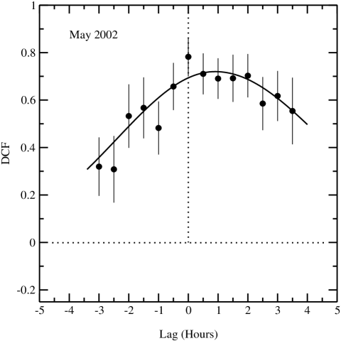
Figure 7: The Discrete Correlation Function between the $B$ and $I$ band light curves during the late May 2002 observations. Significant correlation at positive lags means that the $B$ band variations are leading the $I$ band. The solid line shows the best fitting Gaussian model to the data.

If indeed the observed variability in late May 2002 observations propagates from higher to lower frequencies, we should expect to observe delays between the $B$ and $I$ light curves, with the $B$ band variability leading the $I$ band variations. In order to investigate this issue, we estimated the discrete correlation function (DCF) of the the $B$ and $I$ light curves, using the May 28, 29 and 30, 2002 data, and the method of Edelson & Krolik (1988). The DCF is shown in Fig. 7. The maximum DCF value is $\sim 0.7-0.8$, which indicates that the two light curves are highly correlated. This is not surprising given the very good agreement between the two light curves (Fig. 3). In order to quantify the delay between the light curves (i.e. the lag at which the maximum DCF occurs, $k_{max}$), we fitted the DCF with a Gaussian (the best fitting model is shown with the solid line in Fig. 7). The best fitting $k_{max}$ value is $0.9\pm 1.0$ hrs. The uncertainty corresponds to the $90\%$ confidence limit, and was estimated using the Monte Carlo techniques of Peterson et al. (1998). This result indicates that there is a delay between the $B$ and $I$ band variations, in the expected direction, although not statistically significant. Nevertheless, Fig. 7 shows clearly that the DCF is highly asymmetric towards positive lags. This asymmetry suggests that the $I$ band light curve is indeed delayed with respect to the $B$ band light curve, although in a rather complicated way.

We conclude that, if the May 2002light curves are part of the same flaring event, the observed variations are probably caused perturbations which activate the energy distribution of the particles in the jet. The fact that the rising time scales are steeper in the $B$ band light curves and the DCF asymmetry towards positive lags imply that the injection time scales are very short and that the variations are governed by the cooling time scale of the relativistic particles and the light crossing time scale.

The variability that we observe in May 2002 is qualitatively similar to the variability observed in the short term, optical light curves of BL Lac itself (Papadakis et al. 2003). Just like BL Lac, S4 0954+658 is a classical radio selected BL Lac, whose spectral energy distribution shows a peak at frequencies below the optical band (e.g. Raiteri et al. 1999). Therefore, the optical band corresponds to frequencies located above the peak of the synchrotron emission in this object. We believe that our results demonstrate that well sampled, multi-band optical, intra-night observations of BL Lac objects, whose peak of the emitted power is at mm/IR wavelengths can offer us important clues on the acceleration and cooling mechanism of the particles in the highest energy tail of the synchrotron component.

The present observations are not long enough in order to define accurately the characteristic time scales of the variability processes in action in S4 0954+658. Longer, continuous monitoring of the source, with the collaboration of more than one observatory is needed to this aim. We hope that the results of this work, will motivate the collaboration between the various observatories towards this direction.

- (1) Bevington, P.R. 1969, Data Reduction and Error Analysis for the Physical Sciences. (New York: McGraw-Hill)
- (2) Cardelli, J.A., Clayton, G.C., & Mathis, J.S. 1989, ApJ, 345, 245
- (3) Chiaberge, M., & Ghisellini, G. 1999, MNRAS, 306, 551
- (4) Edelson, R.A., & Krolik, J.H. 1988, ApJ, 333, 646
- (5) Ghisellini, G. et al. 1997, A&A, 327, 61
- (6) Kirk, J.G., Rieger, E.M., & Mastichiadis, A. 1998, A&A, 333, 452
- (7) Papadakis, I.E., Boumis, P., Samaritakis, V., Papamastorakis, J. 2003, A&A, 397, 565
- (8) Peterson, B.M., Wanders, I., Horne, K., Collier, S., Alexander, T., Kaspi, S., & Maoz, D. 1998, PASP, 110, 660
- (9) Raiteri, C. M. et al. 1999, A&A, 352, 19
- (10) Ryter, C.E. 1996, Ap&SS, 236, 285
- (11) Sambruna, R., Maraschi, L., & Urry, M.C., 1996, ApJ, 463, 444
- (12) Scarpa, R., Urry, C.M., Falomo, R., Pesce, J.E., & Treves, A. 2000, ApJ, 532, 740
- (13) Schlegel, D.J., Finkbeiner, D.P., & Davis, M.1998, ApJ, 500, 525
- (14) Wagner, S. J., Sanchez-Pons, F., Quirrenbach, A. & Witzel, A. 1990, A&A, 235, L1
- (15) Wagner, S. J.,Witzel, A., Krichbaum, T. P., Wegner, R., Quirrenbach, A., Anton, K., Erkens, U., Khanna, R. & Zensus, A. 1993, A&A, 271, 344
- (16) Urry, C.M., Sambruna, R.M., Worrall, D.M., Kollgaard, R.I., Feigelson, E. D., Perlman, E. S., & Stocke, J.T. 1996, ApJ, 463, 424