Dark Energy Probes in Light of the CMB

Abstract

CMB observables have largely fixed the expansion history of the universe in the deceleration regime and provided two self-calibrated absolute standards for dark energy studies: the sound horizon at recombination as a standard ruler and the amplitude of initial density fluctuations. We review these inferences and expose the testable assumptions about recombination and reionization that underly them. Fixing the deceleration regime with CMB observables, deviations in the distance and growth observables appear most strongly at $z=0$ implying that accurate calibration of local and CMB standards may be more important than redshift range or depth. The single most important complement to the CMB for measuring the dark energy equation of state at $z\sim 0.5$ is a determination of the Hubble constant to better than a few percent. Counterintuitively, with fixed fractional distance errors and relative standards such as SNe, the Hubble constant measurement is best achieved in the high redshift deceleration regime. Degeneracies between the evolution and current value of the equation of state or between its value and spatial curvature can be broken if percent level measurement and calibration of distance standards can be made at intermediate redshifts or the growth function at any redshift in the acceleration regime. We compare several dark energy probes available to a wide and deep optical survey: baryon features in galaxy angular power spectra and the growth rate from galaxy-galaxy lensing, shear tomography and the cluster abundance.

Kavli Institute for Cosmological Physics, Enrico Fermi Institute and Department of Astronomy and Astrophysics, Chicago IL 60637 USA

1. Introduction

Originating mainly from high redshift, CMB observables provide few direct constraints on the dark energy. Nonetheless, their indirect impact on other more local dark energy probes is important to bear in mind when planning future studies. CMB observables provide two things for dark energy probes: internally or self-calibrated standard rulers and fluctuations for distance and growth rate probes and an expansion history for the universe that is fixed as a function of redshift beyond the current acceleration regime.

We begin in §2. by reviewing the dark energy observables themselves. In §3., we discuss the calibration of the CMB standards and the means by which their self-consistency may be checked. We illustrate these considerations with the recombination calculation. Although the state-of-the-art in recombination is sufficient compared to current measurement errors, it will introduce substantial systematic errors for experiments that are cosmic variance limited out to multipoles of $\ell\sim 10^{3}$ like Planck. Errors in the assumed recombination, including exotica such as a variation in the fine structure constant, would appear as an inconsistency in the damping tail. Accepting the standard thermal history the expansion history is fixed in the deceleration regime. In §4. we explore the implications for dark energy probes. In light of the CMB, the focus returns to low redshift dark energy observables and accurate local calibration. In §5., we consider several optically based probes of the dark energy in light of the CMB.

2. Standard Parameterizations

On scales well below current horizon or Hubble distance where the dark energy can be taken to be smooth, all of its observable effects come through the evolution of its average density $\rho_{\rm DE}(a)$ as a function of scale factor $a=(1+z)^{-1}$. This evolution in turn is related by energy conservation

$$\rho_{\rm DE}(a)=\Omega_{\rm DE}\rho_{\rm crit}\Big{|}_{a=1}e^{-3{\int(1+w)d\ln a}}\,,$$ (1)

to its current energy density $\Omega_{\rm DE}$ relative to critical $\rho_{\rm crit}(a)={3H(a)^{2}/8\pi G}$ and its equation of state

$$p_{\rm DE}(a)=w(a)\rho_{\rm DE}(a)\,.$$ (2)

Hereafter when an argument to $\Omega_{\rm DE}$ and $\rho_{\rm crit}$ is unspecified, $a=1$ is to be understood. We employ throughout units where $c=\hbar=1$.

The two basic dark-energy dependent observables are distance and growth rate. Distance measures are based on having standardized candles, rulers, or object number densities as a function of redshift; growth rate measures are based on standard density fluctuations in linear theory either calibrated today or at the initial conditions and then observed at different redshifts. All distance measures are ultimately based on the comoving distance to redshift $z_{i}$

$$D_{i}\equiv\int_{a_{i}}^{1}{da\over a^{2}H(a)}=\int_{0}^{z_{i}}{dz\over H(z)}\,.$$ (3)

For example, the physical angular diameter distance and luminosity distance are related to the comoving angular diameter distance

$${\cal D}_{i}=R\sin(D_{i}/R)$$ (4)

by multiplying and dividing by $a_{i}$ respectively. Here $R=H_{0}^{-1}(\Omega_{\rm T}-1)^{-1/2}$ is the radius of curvature in an open or closed geometry and $\Omega_{\rm T}\approx\Omega_{m}+\Omega_{\rm DE}$ is the total energy density relative to critical. For comoving distances much smaller than the curvature scale ${\cal D}_{i}\rightarrow D_{i}$. The comoving volume element employed in number density tests is $dV={\cal D}_{i}^{2}dDd\Omega={\cal D}_{i}^{2}(dz/H_{i})d\Omega$ where $d\Omega$ is the solid angle. If the absolute brightness or physical scale of the standards is unknown then a $z_{0}\rightarrow 0$ vs $z_{i}$ comparison will yield the distance ratio

$${{\cal D}_{i}\over{\cal D}_{0}}z_{0}\rightarrow H_{0}{\cal D}_{i}\,,$$ (5)

i.e. a distance measured in units of $h^{-1}$ Mpc. This distinction differentiates (absolute) CMB calibration standards from (relative) local standards. Likewise, if the standard ruler is employed in the radial or redshift direction, it measures $dD/dz=H^{-1}$ if absolutely calibrated and $H_{0}dD/dz=(H_{0}/H)$ if relatively calibrated. Finally the ruler need not even be standard in redshift if its angular and radial extent are compared at the same redshift (Alcock & Paczynski 1979). In this case the quantity measured is $H{\cal D}$.

Under the assumption that the density perturbations are dominated by fluctuations in the non-relativistic matter $\delta_{m}\equiv\delta\rho_{m}/\rho_{m}$, they evolve under self-gravity as

$${d^{2}\delta_{m}\over dt^{2}}+2H(a){d\delta_{m}\over dt}=4\pi G\rho_{m}(a)\delta_{m}\,.$$ (6)

The growth rate is more usefully represented in terms of the scale factor and relative to the rate during the matter dominated epoch. Defining the growth rate $G(a)\propto\delta_{m}/a$, Eqn. (6) becomes

$$\frac{d^{2}G}{d\ln a^{2}}+\left(4+{d\ln H\over d\ln a}\right)\frac{dG}{d\ln a}+\left[3+{d\ln H\over d\ln a}-{3\over 2}\Omega_{m}(a)\right]G=0\,.$$ (7)

For the growing mode of density perturbations one solves this equation with initial conditions of $G=1$ and $dG/d\ln a=0$. Under the assumption of a flat universe, $\Omega_{m}(a)+\Omega_{\rm DE}(a)=1$, $G$ is solely a function of the dark energy density

$$\frac{d^{2}G}{d\ln a^{2}}+\left[\frac{5}{2}-\frac{3}{2}w(a)\Omega_{\rm DE}(a)\right]\frac{dG}{d\ln a}+\frac{3}{2}[1-w(a)]\Omega_{\rm DE}(a)G=0\,.$$ (8)

During the matter dominated epoch $\Omega_{\rm DE}\rightarrow 0$ and $G=$ const. solves the equation of motion. Eqn. (8) is actually correct in general relativistic perturbation theory out to the sound horizon of the dark energy with the generalization that $G$ is the decay rate of the gravitational potential $\Phi\propto G$ in Newtonian gauge (Eisenstein & Hu 1999).

A completely empirical description of the dark energy would require that observations constrain a free function $w(a)$. However, the dark energy will typically only have observable effects during the recent few e-foldings when it contributes substantially to the expansion rate. During this short period in the expansion history, the equation of state function can be usefully approximated through a linear expansion around a normalization epoch $a_{n}$ through the local slope $w_{a}=-dw/da|_{a_{n}}$ as

$$w(a)=w_{n}+(a_{n}-a)w_{a}\,.$$ (9)

As pointed out by Linder (2003), this expansion is more stable to extrapolation away from $a_{n}$ than the analogous linearization in redshift. A common choice for the normalization point in the literature is the present epoch $a_{n}=1$. In this case, let us define the amplitude $w_{0}\equiv w_{n}$, the equation of state parameter today. While we follow this convention here, it is well known that this choice will cause a degeneracy between the amplitude $w_{0}$ and evolution $w_{a}$ of $w(a)$ for typical observables. Thus when marginalized over $w_{a}$, the parameter $w_{0}$ will have large errors. Large errors does not mean that that the equation of state parameter is nowhere well-determined, it simply means that given the possibility of evolution its current value is not well determined. Note that a measurement of $w\neq-1$ at any redshift would rule out a cosmological constant as the dark energy.

A given set of phenomena will best constrain $w$ at the redshifts relevant to the phenomena. It would thus be better to place $a_{n}$ near the expected epoch of dark energy domination. This situation is completely analogous to choosing a scale for the normalization of the power spectrum, e.g. one would not quote a COBE-style horizon scale normalization at $k=H_{0}$ for the WMAP data but a much smaller scale of $k\sim 0.02-0.1$ Mpc^-1 corresponding to the scale of the acoustic peak measurements [see Eqn. (30)].

As with the power spectrum normalization, an inappropriate choice for the dark energy normalization point can be corrected after the fact if the covariance matrix of the parameters is also given. Suppose one analyzes the data with a dark energy parameterization of $p=(w_{0},w_{a})$ then the covariance matrix of an alternate choice $p^{\prime}=(w_{n},w_{a})$ is given by the Jacobian transformation

$$C_{\mu\nu}^{\prime}=\sum_{\alpha\beta}{\partial p_{\alpha}^{\prime}\over\partial p_{\mu}}C_{\alpha\beta}{\partial p_{\beta}^{\prime}\over\partial p_{\nu}}\,.$$ (10)

In particular, there is a “best” choice for a given observation (Eisenstein et al. 1999b; Hu & Jain 2003)

$${a_{n}}={a_{\rm pivot}}\equiv{C_{w_{0}w_{a}}\over C_{w_{a}w_{a}}}+1\,,$$ (11)

such that the errors on $w_{\rm pivot}$ and $w_{a}$ are uncorrelated. Furthermore the errors on $w_{\rm pivot}$ are the same as that on $w_{0}$ with the evolution $w_{a}$ fixed by a prior. To avoid confusion however, we will refer to constraints in the context of a constant $w$ as being on the quantity

$$w_{\rm DE}=w(a)={\rm const.}$$ (12)

The distinction between $w_{\rm pivot}$ and $w_{\rm DE}$ arises when considering multidimensional constraints. For example in the 2D ($\Omega_{\rm DE}$,$w_{\rm DE}$) plane, errors in the $\Omega_{\rm DE}$ direction increase due to marginalization over $w_{a}$.

3. CMB Standards

CMB standards for the dark energy are particularly useful in that they are internally or self-calibrated. Equally importantly, the physical processes governing these standards are sufficiently simple that there are only a few assumptions going into the calibration. These assumptions can themselves be tested through internal consistency checks.

These standards are mainly based on the acoustic features in the power spectrum of CMB anisotropies. These features are frozen in place at recombination. The theoretical accuracy to which we can calibrate these standards is limited by the accuracy to which recombination has been calculated.

3.1. Recombination Aside

The accuracy of CMB anisotropy calculations are limited not by that of the radiative transfer or the general relativistic description but ironically by that of the recombination calculation. This status has been true at least since the development of the modern Einstein-Boltzmann codes in the mid 1980’s when radiative transfer improvements began to outpace recombination improvements. The currently claimed $0.1\%$ precision of numerical codes (Seljak et al. 2003) is just that: a statement of precision. The accuracy of the standard recombination calculation has only been certified to the $\sim 1\%$ level.

The current standard for calculating the ionization history is RECFAST (Seager et al. 1999) which employs the traditional two-level atom calculation of Peebles (1968) but alters the hydrogen case $B$ recombination rate $\alpha_{B}$ to fit the results of a multilevel atom. More specifically, RECFAST solves a coupled system of equations for the ionization fraction $x_{i}$ in singly ionized hydrogen and helium ($i=$ H, He)

$${dx_{i}\over d\ln a}={\alpha_{B}C_{i}n_{H}\over H}\left[s(x_{\rm max}-x_{i})-x_{i}x_{e}\right]\,,$$ (13)

where $n_{H}=(1-Y_{p})n_{b}$ is the total hydrogen number density accounting for the helium mass fraction $Y_{p}$, $x_{e}\equiv n_{e}/n_{H}=\sum x_{i}$ is the total ionization fraction, $n_{e}$ is the free electron density, $x_{\rm max}$ is the maximum $x_{i}$ achieved through full ionization,

$$s={\beta\over n_{H}}e^{-B_{1s}/k_{B}T_{b}}\,,\quad C_{i}^{-1}=1+{\beta\alpha_{B}e^{-B_{2s}/k_{B}T_{b}}\over\Lambda_{\alpha}+\Lambda_{2s1s}}\,,\quad\beta=g_{\rm rat}\left({k_{B}T_{b}m_{e}\over 2\pi\hbar^{2}}\right)^{3/2}\,,$$ (14)

with $g_{\rm rat}$ the ratio of statistical weights, $T_{b}$ the baryon temperature, $B_{L}$ the binding energy of the $L$th level, $\Lambda_{\alpha}$ the rate of redshifting out of the Lyman-$\alpha$ line corrected for the energy difference between the $2s$ and $2p$ states

$$\Lambda_{\alpha}={1\over\pi^{2}}\left({B_{1s}-B_{2p}\over\hbar c}\right)^{3}e^{-(B_{2s}-B_{2p})/k_{B}T_{b}}{H\over(x_{\rm max}-x_{i})n_{H}}$$ (15)

and $\Lambda_{2s1s}$ as the rate for the 2 photon $2s-1s$ transition. For reference, for hydrogen $B_{1s}=13.598$eV, $B_{2s}=B_{2p}=B_{1s}/4$, $\Lambda_{2s1s}=8.22458s^{-1}$, $g_{\rm rat}=1$, $x_{\rm max}=1$. For helium $B_{1s}=24.583$eV, $B_{2s}=3.967$eV, $B_{2p}=3.366$eV, $\Lambda_{2s1s}=51.3s^{-1}$, $g_{\rm rat}=4$, $x_{\rm max}=Y_{p}/[4(1-Y_{p})]$.

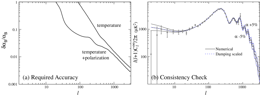
Figure 1.: Recombination and the accuracy of CMB calibrations. (a) The current state-of-the-art in recombination involves a calibrated fudge in rescaling $\alpha_{B}$ for hydrogen in a 2 level atom to a multilevel atom. Shown is precision to which $\alpha_{B}$ will need to be calibrated so as to not introduce systematic errors that are larger than the cosmic variance out to a given $\ell$. (b) The damping tail contains a consistency check for recombination, here illustrated through a 5% variation in the fine structure constant $\alpha$ or a $\sim 10\%$ variation in $z_{*}$. The first 3 peaks measured by WMAP (points) determines the photon-baryon ratio $R_{*}$ and radiation matter ratio $r_{*}$ at recombination, here held fixed. The damping tail breaks the degeneracy and measures $z_{*}$ independently, here accurately analytically modeled through a change in the damping scale (dashed lines).

If $\alpha_{B}C_{i}n_{H}/H\gg 1$, the $x_{i}$ reaches the Saha equilibrium, $s(x_{\rm max}-x_{i})=x_{i}x_{e}$ or

$$x_{i} = {1\over 2}\left[\sqrt{(x_{ei}+s)^{2}+4sx_{\rm max}}-({x_{ei}+s})\right]$$

$$= x_{\rm max}\left[1-{x_{ei}+x_{\rm max}\over s}\left(1-{x_{ei}+2x_{\rm max}\over s}\right)+...\right]\,,$$

where $x_{ei}=x_{e}-x_{i}$ is the ionization fraction excluding the species. This solution is used in place of the integration until say $x_{i}/x_{\rm max}-1=10^{-3}$. The recombination of hydrogenic doubly ionized helium is handled purely through the Saha equation with a binding energy of ${1/4}$ the $B_{1s}$ of hydrogen and $x_{\rm max}=Y_{p}/[4(1-Y_{p})]$. The case $B$ recombination coefficients as a function of $T_{b}$ are given in Seager et al. (1999) as is the strong thermal coupling between $T_{b}$ and $T_{\rm CMB}$. The multilevel-atom fudge that RECFAST introduces is to replace the hydrogen $\alpha_{B}\rightarrow 1.14\alpha_{B}$ independently of cosmology.

While this fudge suffices for the current observations, the recombination standard will require improvement if CMB anisotropy constraints are to reach their full potential. To estimate at what point the recombination calculation will need to be improved we can compare the sensitivity of the spectra to the $\alpha_{B}$ fudge to cosmic variance errors. Fig. 1 shows that at $\ell>1000$ a calibration to the multilevel atom that is better than the current 1% level in $\alpha_{B}$ will be required. Furthermore there is no guarantee that the $\alpha_{B}$ fudge will work to this level of precision.

Fortunately the higher acoustic peaks provide a built in self-consistency test of recombination. Since the recombination rate $\alpha_{B}$ has been downgraded from a physical parameter to a fitting parameter, a more physically interesting way to phrase the sensitivity is to change recombination through the fine structure constant $\alpha$. In the recombination calculation, all of the binding energies scale as $B\propto\alpha^{2}$, $\Lambda_{2s1s}\propto\alpha^{8}$ and (Kaplinghat et al. 1999)

$$\alpha_{B}\propto\alpha^{2(1-\partial\ln\alpha_{B}/\partial\ln T_{b})}\,.$$ (17)

In addition $\sigma_{T}\propto\alpha^{2}$.

The phenomenology of the CMB is primarily governed by the redshift of recombination $z_{*}=a_{*}^{-1}-1$ though that dependence is largely hidden in standard recombination by its insensitivity to the usual cosmological parameters. This insensitivity and the sensitivity to $\alpha$ follows from the fact that recombination proceeds rapidly once $B_{1s}/kT_{b}$ has reached a certain threshold. Defining the redshift of recombination as the epoch at which the Thomson optical depth during recombination (i.e. excluding reionization) reaches unity, $\tau_{\rm rec}(z_{*})=1$, a fit to the recombination calculation gives

$$\begin{array}[]{rcl}a_{*}^{-1}&=&1047.5[1+0.00124(\Omega_{b}h^{2})^{-0.738}][1+b_{1}(\Omega_{m}h^{2})^{b_{2}}]\left({\alpha\over\alpha_{0}}\right)^{2.08},\\ b_{1}&=&0.0783(\Omega_{b}h^{2})^{-0.238}[1+39.5(\Omega_{b}h^{2})^{0.763}]^{-1},\\ b_{2}&=&0.560[1+21.1(\Omega_{b}h^{2})^{1.81}]^{-1}\,,\end{array}$$ (18)

where $\alpha_{0}\approx 1/137$, the fine structure constant from laboratory measurements today. The sensitivity to cosmological parameters is weak. Around the fiducial model of $\Omega_{m}h^{2}=0.14$ and $\Omega_{b}h^{2}=0.024$, the recombination redshift becomes

$$a_{*}^{-1}\approx 1089\left({\Omega_{m}h^{2}\over 0.14}\right)^{0.0105}\left({\Omega_{b}h^{2}\over 0.024}\right)^{-0.028}\left({\alpha\over\alpha_{0}}\right)^{2.08}\,.$$ (19)

However one cannot translate the typical CMB constraints on $z_{*}$, $\Omega_{b}h^{2}$ and $\Omega_{m}h^{2}$ into constraints on $\alpha$ since the values of all three are determined in the context of standard recombination. We shall now see how constraints from acoustic phenomena arise in a general context.

3.2. Standard Rulers

The CMB acoustic peaks are governed by 4 physical quantities: the photon-baryon ratio, the matter-radiation ratio, the sound horizon, and the diffusion scale all evaluated at the epoch of recombination. In the standard thermal history context, the photon and neutrino densities are fixed by the measurement of the CMB temperature and $T_{\nu}=(4/11)^{1/3}T_{\rm CMB}$. Defining $T_{\rm rat}=T_{\rm CMB}/2.725$K, the photon-baryon ratio becomes

$$R_{*}\equiv{3\over 4}{\rho_{b}\over\rho_{\gamma}}\Big{|}_{a_{*}}=0.729\left({\Omega_{b}h^{2}\over 0.024}\right)\left({a_{*}\over 10^{-3}}\right)T_{\rm rat}^{-4}\,,$$ (20)

and the radiation-matter ratio becomes

$$r_{*}\equiv{\rho_{r}\over\rho_{m}}\Big{|}_{a_{*}}=0.297\left({\Omega_{m}h^{2}\over 0.14}\right)^{-1}\left({a_{*}\over 10^{-3}}\right)^{-1}T_{\rm rat}^{4}\,.$$ (21)

Moreover for standard recombination $z_{*}$ itself is only a weak function of $\Omega_{b}h^{2}$ and $\Omega_{m}h^{2}$ [see Eqn. (19)] and so a measurement of $R_{*}$ and $r_{*}$ translate directly into a measurement of $\Omega_{b}h^{2}$ and $\Omega_{m}h^{2}$. Conversely, constraints on these two quantities can be generalized to a broader context with these relations. In Fig. 1b the result of 5% variations in $\alpha$ and hence $\sim 10\%$ variations in the redshift of recombination are shown. The variations are taken at fixed $R_{*}$ and $r_{*}$ and hence $\Omega_{b}h^{2}$ and $\Omega_{m}h^{2}$ that vary by $\sim 10\%$. In the region of the first 3 peaks, these models produce nearly identical spectra. Hence in the general context it is $R_{*}$ and $r_{*}$ that the CMB measures not $\Omega_{b}h^{2}$ and $\Omega_{m}h^{2}$ directly.

In terms of the physics of the peaks, $R_{*}$ controls the baryon loading of the fluid and $r_{*}$ controls the depths of the gravitational potentials (see e.g. Hu et al. 2000). In terms of the phenomenology, baryon loading in gravitational potential wells modulates the relative heights of the odd and even numbered peaks whereas the depths of the gravitational potential wells themselves also control the amplitude envelope of all of the peaks.

With measurements of $R_{*}$ and $r_{*}$ from the morphology of the peaks, the overall physical scale associated with the acoustic phenomena is self-calibrated under standard recombination. This is the distance sound can travel by recombination

$$s_{*} = \int_{0}^{a_{*}}{da\over a^{2}H(a)}c_{s}(a)$$ (22)

$$= {2\sqrt{3}\over 3}\sqrt{a_{*}\over R_{*}\Omega_{m}H_{0}^{2}}\ln{\sqrt{1+R_{*}}+\sqrt{R_{*}+r_{*}R_{*}}\over 1+\sqrt{r_{*}R_{*}}}\qquad{\rm MD/RD}$$

where the sound speed $c_{s}=1/\sqrt{3(1+R)}$ and the second line assumes that only matter and radiation are important in $H(a)$ before recombination. Around the fiducial model,

$${s_{*}\over{\rm Mpc}}\approx 144.4\left({\alpha\over\alpha_{0}}\right)^{-1.36}\left({\Omega_{m}h^{2}\over 0.14}\right)^{-0.252}\left({\Omega_{b}h^{2}\over 0.024}\right)^{-0.083}\,.$$ (23)

Therefore, in the standard recombination context where $\alpha=\alpha_{0}$, the CMB provides an absolutely calibrated (in Mpc, not $h^{-1}$ Mpc) standard ruler for cosmology. More generally the standard ruler carries a scaling factor of $(a_{*}/\Omega_{m}h^{2})^{1/2}$ if only $R_{*}$ and $r_{*}$ are determined. This standard thermal history assumption is important to bear in mind when using this standard ruler for dark energy tests.

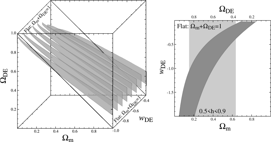
Figure 2.: Generalizing the sound horizon dark energy constraint. Given CMB constraints on the acoustic scale $\ell_{A}$, $\Omega_{m}h^{2}$ and $\Omega_{b}h^{2}$, CMB constraints can be applied to any set of dark energy parameters by propagation of errors. Shown here are WMAP constraints (a) in a 3D space of $\Omega_{m}$, $\Omega_{\rm DE}$, and $w_{\rm DE}$ and (b) projected onto the usual space of flat cosmologies.

CMB constraints implicitly use this standard ruler in a distance measure test for dark energy. The sound horizon sets the fundamental physical scale of the peaks which is then measured in angular or multipole space as

$$\ell_{A}={\pi{\cal D}_{*}\over s_{*}}\,.$$ (24)

With the absolute calibration of $s_{*}$, the CMB then measures the angular diameter distance ${\cal D}_{*}$ to recombination in absolute units. Note that even though the standard parameter analyses usually assume a simple dark energy model when calculating constraints, they may be readily translated into a general context by error propagation. In Fig. 2 we show an example where WMAP errors on $\ell_{A}=299\pm 2$, $\Omega_{m}h^{2}=0.14\pm 0.02$ and $\Omega_{b}h^{2}=0.024\pm 0.002$ (Spergel et al. 2003) are used to delimit a region in the three dimensional distance measure space of curvature, constant $w_{\rm DE}$ and $\Omega_{\rm DE}$.

For quick estimation purposes or a poor-man’s MCMC, note that the dominant source of error in the sound horizon calibration is from $\Omega_{m}h^{2}$ and that the measurement errors on $\ell_{A}$ are comparatively small. (In fact ever since the first crude detection of the first peak in 1999 errors in the dark energy–curvature domain have been dominated by those in $\Omega_{m}h^{2}$ and not by the precision with which $\ell_{A}$ was measured. Before self-calibration became available from the higher peaks this was phrased in terms of the prior on $h$.) As a rule of thumb, Eqn. (23) implies the errors on the distance to recombination scale as

$$\sigma(\ln{\cal D}_{*})\approx{1\over 4}\sigma(\ln\Omega_{m}h^{2})\,.$$ (25)

For example WMAP quotes errors of 14% in $\Omega_{m}h^{2}$ and $3.6\%$ in ${\cal D}_{*}$ (Spergel et al. 2003). Improving the distance measure and the calibration of the standard ruler $s_{*}$ thus is best achieved by accurately measuring the 3rd and higher acoustic peaks.

Beyond the third peak in the temperature, the CMB can test the internal consistency of the standard thermal history. The damping of the acoustic peaks is associated with the radiative transfer or diffusion of the CMB photons during recombination. Under standard recombination, the diffusion distance is uniquely determined by the baryon and matter densities $\Omega_{b}h^{2}$ and $\Omega_{m}h^{2}$ and presents another absolutely calibrated standard ruler. However a change in the thermal history that delays recombination will allow the photons to diffuse further (Peebles et al. 2000) even if the dynamics in the tight coupling regime is held fixed by keeping $R_{*}$ and $r_{*}$ the same. In Fig. 1b we see that models with a recombination variation due to $\alpha$ start to differ at the third peak.

Given a thermal history, the damping effect can be quantified via Boltzmann techniques given in Hu & White (1997). The result is that the damping scale can be approximated by

$$\lambda_{D}=15.96{a_{*}^{1.1}R_{*}^{-0.23}\over\sqrt{\Omega_{m}^{0.78}\Omega_{b}^{0.22}H_{0}^{2}}}(1+1.105R_{*}^{1.87})^{1/5}[(1+r_{*})^{1/2}-r_{*}^{1/2}]^{1/2}\,.$$ (26)

In comparison to the acoustic scale, the damping scale has a stronger dependence on the redshift of recombination and the baryons. Around the fiducial model it is approximately

$${\lambda_{D}\over{\rm Mpc}}\approx 64.5\left({\alpha\over\alpha_{0}}\right)^{-7/3}\left({\Omega_{m}h^{2}\over 0.14}\right)^{-0.278}\left({\Omega_{b}h^{2}\over 0.024}\right)^{-0.18}\,.$$ (27)

This scale is also projected onto angle via the angular diameter distance

$$\ell_{D}={2\pi{\cal D}_{*}\over\lambda_{D}}$$ (28)

and appears in the power spectrum as a sharp damping of the acoustic amplitude by

$${\cal D}_{\ell}\approx\exp[-(\ell/\ell_{D})^{1.25}]\,.$$ (29)

The ratio of the two scales $\ell_{D}/\ell_{A}$ (essentially the number of observable peaks) is independent of the distance and dark energy and hence tests the assumptions entering into the calibration of the standard rulers.

In Fig. 1b (dashed lines) we rescale the power spectrum of the fiducial model to the $\ell_{D}$ of the varying $\alpha$ models by multiplying by the ratio of ${\cal D}_{\ell}^{2}$. The good agreement explicitly demonstrates that aside from damping, the morphology of the acoustic peaks is preserved at fixed $R_{*}$ and $r_{*}$.

In summary the damping scale and the associated polarization is a consistency check on the standard thermal history assumptions. Under these assumptions both are uniquely predicted by the low order temperature peaks. Problems with the assumptions on the recombination history, e.g. the fine structure constant or a more prosaic problem with the multilevel hydrogen atom would manifest themselves here. Likewise problems in the assumption of the radiation density, e.g. a change in the number or temperature of the neutrinos, would show up here due a change in the damping scale relative to the acoustic scale and also due to effects from their anisotropic stress. Finally any contamination from secondary anisotropies and point sources would show up more strongly here. Current small scale anisotropy and polarization data is in good agreement with the predictions from the first three peaks. These consistency tests provide more confidence that the sound horizon is both an internally calibrated and internally consistent standard ruler that can be used for dark energy probes, at least to the current level of precision in the standard.

3.3. Standard Fluctuations

The CMB also provides a calibration standard for dark energy and/or massive neutrino growth rate tests. The height of the acoustic peaks is now very well calibrated (Page et al. 2003) and in conjunction with the well understood radiation transfer described in the previous sections, it can be converted into a measurement of the initial amplitude of fluctuations.

For illustrative purposes, we will here assume that the neutrino masses are negligible. The initial spectrum of curvature fluctuations $\zeta$

$$\Delta_{\zeta}^{2}\equiv{k^{3}\over 2\pi^{2}}P_{\zeta}(k,a_{i})=\delta_{\zeta}^{2}\left({k\over k_{n}}\right)^{n-1}\,,$$ (30)

is processed through the radiation transfer to become the CMB power spectra and matter power spectrum. Here $k_{n}$ is the normalization scale and we will follow the WMAP convention of choosing $k_{n}=0.05$ Mpc^-1. Note that the actual pivot point or best constrained normalization point for WMAP is closer to $k_{n}=0.02$ Mpc^-1 corresponding to the first peak. The amplitude of fluctuations from WMAP is

$$\delta_{\zeta}\approx 5.07e^{-(0.17-\tau)}\times 10^{-5}\,,$$ (31)

or equivalently in terms of the WMAP normalization parameter

$$A=(1.84\delta_{\zeta}\times 10^{4})^{2}=0.87e^{-2(0.17-\tau)}\,.$$ (32)

If taken instead as the amplitude at the pivot point, the uncertainties in $\delta_{\zeta}$ come almost entirely from that in the optical depth $\tau$; with the fiducial choice there is a small increase in the uncertainties due to the constraint on the tilt. In any case the amplitude of the initial fluctuations is known to better than 10% at scales relevant to large-scale structure. This calibration exceeds the accuracy to which the normalization of the power spectrum at the current epoch is known. Thus for dark energy tests involving the growth of structure, it is already advantageous to compare high redshift structure to the CMB normalization instead of the local normalization. In addition, a measurement of the local $z=0$ normalization also becomes a test of the dark energy.

The matter power spectrum is processed through the same radiation transfer as the CMB and so the latter determines the former. In the standard cosmology this is reflected in the fact that the transfer function when expressed in Mpc^-1 depends only on the well determined $\Omega_{b}h^{2}$ and $\Omega_{m}h^{2}$. Thus both the shape and the normalization of the matter power spectrum in the deceleration epoch is fixed in physical units of Mpc.

The amplitude at $z=0$ then becomes a measure of the dark energy. It is usually quoted in terms of the rms of the linear density field smoothed by a tophat of radius $r=8h^{-1}$Mpc (Hu & Jain 2003)

$$\sigma_{8}^{2} \equiv \int{dk\over k}\Delta_{m}^{2}(k,a=1)W_{\sigma}^{2}(kr)$$

$$\sigma_{8} \approx {\delta_{\zeta}\over 5.59\times 10^{-5}}\left({\Omega_{b}h^{2}\over 0.024}\right)^{-1/3}\left({\Omega_{m}h^{2}\over 0.14}\right)^{0.563}$$ (33)

$$\times(3.123h)^{(n-1)/2}\left({h\over 0.72}\right)^{0.693}{G_{0}\over 0.76}\,,$$

where $W_{\sigma}(x)=3x^{-3}(\sin x-x\cos x)$ is the Fourier transform of a top hat window. $G_{0}=G(a=1)$ the growth function evaluated at the current epoch. Note that because the normalization is given in $h^{-1}$ Mpc, there is a strong scaling with the Hubble constant. In a flat universe $\Omega_{\rm DE}=1-\Omega_{m}$ and precise measurements of $\Omega_{m}h^{2}$ then fix $\Omega_{\rm DE}$ given $h$. We shall see in the next section that the Hubble constant is the single most useful complement to CMB parameters for dark energy studies. Likewise a measurement of $\sigma_{8}$ is a measurement of the specific combination of dark energy parameters above. At high redshift, one replaces $G_{0}\rightarrow G(a)$ in equation (33) and so the measurement of structure as a function of redshift can in principle measure the whole growth function.

In summary, the CMB standard fluctuation is internally calibrated, this time by the large-angle polarization-temperature cross correlation through $\tau$. The inference on $\tau$ will be more thoroughly tested once the polarization auto power spectrum becomes available. Furthermore an independent internal consistency check on this calibration is provided by the gravitational lensing signature in the CMB (Hu 2002; Kaplinghat et al. 2003).

4. Standard Deviants

The CMB has provided two self-calibrated standards for dark energy studies, a standard ruler: the sound horizon at recombination and a standard fluctuation: the initial amplitude of fluctuations at the $k=0.05$ Mpc^-1 scale. Their respective calibration errors are currently $<4\%$ and $<10\%$ respectively. With the sound horizon calibration, the peak locations constrain the distance to the recombination surface to the same fractional accuracy.

With the addition of better small scale anisotropy and large scale polarization measurements one can expect that the statistical errors will further improve by up to a factor of 10. Moreover internal consistency tests should ensure accuracy and test for systematic errors. It is therefore interesting to reconsider the dark energy observables keeping the CMB standards, i.e. the high redshift universe and hence ${\cal D}_{*}$, $G_{*}$, $\Omega_{b}h^{2}$ and $\Omega_{m}h^{2}$ fixed. We shall see that this perspective leads to several counterintuitive results which highlight the importance of accurate local calibration over redshift range or depth.

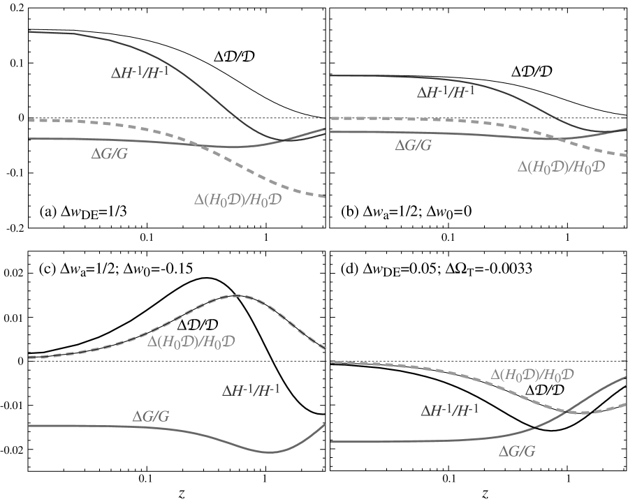
Figure 3.: Deviations in the dark energy observables holding CMB observables ${\cal D}_{*}$ and $G_{*}$ fixed by varying $\Omega_{\rm DE}$ to compensate a variation in (a) a constant $w_{\rm DE}$; (b) $w_{a}=-dw/da$ at fixed $w(a=1)=w_{0}$; compensating variations which leave $H_{0}$ fixed (c) $\Delta w_{a}/\Delta w_{0}\approx-10/3$ (d) $\Delta w_{\rm DE}/\Delta\Omega_{T}\approx-15$. With fixed high-$z$ observables, the main deviations due to the dark energy equation of state appear as variations in the Hubble constant which can be measured at low redshift by absolute standards through ${\cal D}$, $H$ or at high redshift through relative standards $H_{0}{\cal D}$. The local value of the growth function $G_{0}=G(a=1)$ is useful in breaking the degeneracy left by variations at fixed $H_{0}$.

In Fig. 3a we show deviations in the distance and growth dark energy observables from a fiducial model of $\Omega_{\rm DE}=1-\Omega_{m}=0.73$ and $w_{\rm DE}=-1$ (with $\Omega_{m}h^{2}=0.14$ and $\Omega_{b}h^{2}=0.024$). These are the angular diameter distance ${\cal D}$, the Hubble parameter $H$, the growth function $G$ and the combination $H_{0}{\cal D}$, the distance as measured by a comparison of local and high redshift standards. Note that with $\Omega_{m}h^{2}$ fixed, ${\cal D}$ and $H$ are known functions of redshift in the matter dominated or deceleration regime.

Let us begin with a variation of $\Delta w_{\rm DE}=1/3$, i.e. a model with $w_{\rm DE}=-2/3$. Given a fixed ${\cal D}_{*}$, $\Omega_{\rm DE}$ is then not a free parameter but fixed given $w_{\rm DE}$. This is similar to but not equivalent to the usual fixing of $\Omega_{m}$ or $\Omega_{\rm DE}$ by a prior found in SNe forecasts. The CMB prior on ${\cal D}_{*}$ is simple to apply and should be used in any projection involving the CMB (e.g. Hu et al. 1999; Spergel & Starkman 2002; Frieman et al. 2003).

Fixing ${\cal D}_{*}$ changes the perspective on where in redshift the largest deviations from the fiducial $\Lambda$ model would appear. Not surprisingly given that the CMB is a high redshift probe, in terms of absolute distances and growth, it is $z\rightarrow 0$ where most of the effects are largest. In fact the single most useful measurement that would complement the CMB distance measure is a Hubble constant measurement that is accurate to the percent level. Note that at $z\rightarrow 0$ deviations in the Hubble parameter $\Delta H/H$ and the angular diameter distance $-\Delta{\cal D}/{\cal D}$ are given by that in the Hubble constant $\Delta H_{0}/H_{0}$. Likewise, since the dark energy only affects the growth of structure during the acceleration epoch, the deviations in it also appear only at $z\mathrel{\hbox{\hbox to0.0pt{\hbox{\lower 4.0pt\hbox{$\sim$}}\hss}\hbox{$<$}}}1$. Here nearly compensating variations in $w_{\rm DE}$ and $\Omega_{\rm DE}$ imposed by ${\cal D}_{*}$ keep the fractional variations in $G$ small compared with those in $H_{0}$ but recall that redshift survey based measurements of fluctuations carry a strong scaling with $H_{0}$ on top of the growth rate [see Eqn. (33)].

Relative standards that measure $H_{0}{\cal D}$ are an exception to the low redshift rule but not an exception to the $H_{0}$ rule. Here the maximum deviation appear at high-$z$ but since ${\cal D}$ is fixed at high-$z$, $\Delta H_{0}{\cal D}/H_{0}{\cal D}\rightarrow\Delta H_{0}/H_{0}$. In other words, since the distance to high redshift is known, measurement of a standard candle becomes a calibration of the absolute brightness of the standard. Phrased another way, relative standards measure $\Omega_{m}$ in the deceleration regime and when combined with $\Omega_{m}h^{2}$ from the CMB determine $H_{0}$. The CMB provides a counter-intuitive way of measuring the Hubble constant by inverting the distance ladder! Of course in practice, the assumption that the candle is standard or standardize-able between redshift zero and the deceleration epoch is suspect. Note also that Fig. 3a only shows the best epoch to measure the dark energy observables given fixed fractional measurement errors in the observables. It does not factor in the observational cost required to achieve a fixed fractional distance error at high redshift.

These rules of thumb remain valid for deviations involving an evolution in the equation of state from its present value. In Fig. 3b we show the deviations for $\Delta w_{a}=1/2$ with $w_{0}=-1$. Again the same statements apply: the maximal deviations for absolute standards appear at redshift zero and for relative standards at high redshift. For the distance measures, the asymptotic deviations correspond to variations in the Hubble constant.

The deviations due to $w_{0}$ at fixed $w_{a}=0$ (or equivalently $w_{\rm DE}$) and those for $w_{a}$ at fixed $w_{0}$ have similar forms since to leading order they are both tied to uncertainties in the Hubble constant. This similarity implies a degeneracy between $w_{0}$ and $w_{a}$ along a line of $\Delta w_{0}/\Delta w_{a}\approx-3/10$ which holds $H_{0}$ fixed. As noted in §2., a degeneracy between $w_{0}$ and $w_{a}$ simply implies that the equation of state is better constrained at a redshift that differs from $z=0$. In this CMB context with fixed high-$z$ quantities, this implies $a_{\rm pivot}=7/10$ from Eqn. (11) or $z_{\rm pivot}=0.43$ as the epoch at which the dark energy equation of state is best constrained. Recall that a measurement of $w\neq 1$ at any redshift would rule out a cosmological constant. Conversely a confirmation of $w=-1$ at such a redshift would strongly favor a cosmological constant since an alternate solution would require a $w_{a}$ variation that sent the dark energy to a phantom regime $w<-1$ in the past expansion history, or a stronger variation in $w$ that violated the $w_{a}$ linearization.

In Fig. 3c, we plot the deviations along this degeneracy line (deviations are here actually between $w_{0}=-0.85$, $w_{a}=0$ and $w_{0}=-1$, $w_{a}=1/2$ to avoid the phantom dark energy regime). Note the change in scale of the axes. Because this line preserves the Hubble constant, the deviations in ${\cal D}$ and $H_{0}{\cal D}$ now coincide and disappear at both low and high redshift. The Hubble parameter deviations persist until higher redshift and the growth function deviations remain fairly level for $z\mathrel{\hbox{\hbox to0.0pt{\hbox{\lower 4.0pt\hbox{$\sim$}}\hss}\hbox{$<$}}}3$. Note that still a measurement of the growth function locally provides a means of breaking the degeneracy. In any case, any means of breaking the degeneracy left at constant $H_{0}$ will require percent level accuracy in the measurements and calibration of the standards.

Finally these patterns also appear with variations involving the curvature or $\Omega_{T}$. As is well known, variations in the curvature off of a flat cosmology are allowed by the CMB but come at the cost of a change in the Hubble constant. Again an accurate Hubble constant is the key. With $w_{\rm DE}$, a more subtle degeneracy with $\Omega_{T}$ at fixed $H_{0}$ opens up (see Fig. 3d). In this case measurement of the growth function at the present epoch becomes even more important since the distance degenerate increment in $w_{\rm DE}$ and decrement in $\Omega_{T}$ both slow the growth of structure. Note though that at the $1\%$ level in growth rate, massive neutrinos will certainly have to be included in the interpretation and error budget.

In summary, to test the cosmological constant hypothesis and measure the equation of state of the dark energy at $z\sim 0.4-0.5$, the best complement to current and future CMB measurements is a measurement of the Hubble constant that is accurate at the few percent level. Ironically, one way of achieving this is to measure the relative luminosity distance to a redshift in the deceleration regime. If the measurement is inconsistent with a cosmological constant, then to further measure the evolution of $w$ through $w_{a}$ or rule out an alternate explanation involving spatial curvature will require percent level measurement and calibration of standard candles, rulers, number densities at intermediate redshifts or fluctuations at any redshift.

5. Standard Forecasts?

The general considerations of the previous sections can be turned into specific forecasts for dark energy parameters given assumptions about the observations in question: both on the CMB side and on the dark energy probe side. If the observations are expected to constrain the models to live in a small region of parameter space and systematic errors are negligible, then linear propagation of statistical errors, also known as Fisher matrix forecasts, provide a useful guide to their capabilities.

Unfortunately one can make a dark energy parameter forecast give practically any desired answer by adjusting prior assumptions both on the cosmology and the systematic error floor. (First rule of parameter estimation: state your priors. Second rule of parameter estimation: state your priors.) As an exercise, here we will try to compare on an equal footing (when titles end with a question mark, the answer is no) several different dark energy probes that can come out of a deep and wide optical survey. Specifically we assume a multi-color survey that allows binning of galaxies to $\Delta z=0.1$ out to $z=1$ across 4000 deg². We will assume CMB priors that come from a forecast of the Planck satellite assuming only statistical errors in a parameter space that includes $\Omega_{m}h^{2}$, $\Omega_{b}h^{2}$, $n$, $\delta_{\zeta}$, tensors, and $\tau$ as well as the dark energy parameters of interest (Hu 2002). As we have seen in §3., the critical CMB assumptions are on the physical matter density $\sigma(\ln\Omega_{m}h^{2})=0.01$ which controls the calibration of the sound horizon and $\sigma(\tau)=0.005$ which controls the calibration of the growth function. We also assume a spatially flat universe.

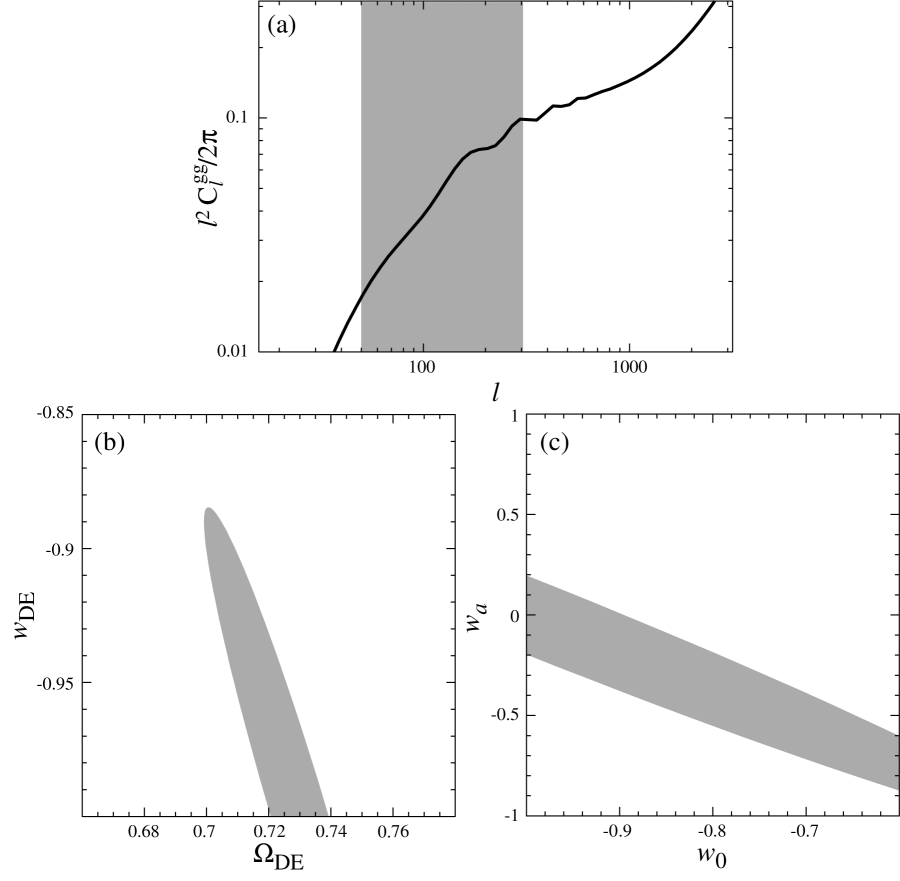
Figure 4.: Acoustic or baryon features in the galaxy angular power spectrum. (a) angular power spectrum at $z=1$ with $\Delta z=0.1$ for galaxies in halos above $M_{\rm th}=10^{12.5}h^{-1}M_{\odot}$; (b) constraints on $w_{\rm DE}$ and $\Omega_{\rm DE}$ from $50\leq\ell\leq 300$ and 10 angular spectra out to $z=1$ with Planck CMB priors; (c) constraints in the $w_{0}-w_{a}$ plane marginalized over $\Omega_{\rm DE}$.

Given that the sound horizon at recombination is already calibrated at the few percent level, its appearance in the matter power spectrum as baryon features or “wiggles” provides a theoretically robust, but observationally challenging, probe of the dark energy (Eisenstein et al. 1999). Much recent work has gone into their utilization in a high-$z$ redshift survey (e.g. Blake & Glazebrook 2003; Hu & Haiman 2003; Seo & Eisenstein 2003).

It is interesting to investigate to what extent a photometric survey can utilize the baryon features. A photometric survey essentially loses all ability to measure the Hubble parameter $H(a)$ directly through the standard ruler in the radial direction unless $\Delta z\ll 0.01$. As a means of measuring the angular diameter distance ${\cal D}$, a photometric survey fairs better (Cooray et al. 2001). At high redshift, the change in the distance per unit redshift is small and even a fairly thick shell of $\Delta z=0.1$ produces very little smearing of the features due to projection. In Fig. 4, we show the angular power spectrum of galaxies in haloes $M\geq M_{\rm th}=10^{12.5}h^{-1}M_{\odot}$ predicted under the halo model described in Hu & Jain (2003). Of course, a measurement of ${\cal D}$ from the angular power spectrum still does not rival that from the 3D power spectrum given the loss of radially directed modes. The relative degradation as a function of redshift resolution can be estimated by a simple mode counting argument (Hu & Haiman 2003).

Still the angular power spectrum does yield some constraint on the dark energy. In Fig. 4, we show the results of a Fisher forecast with 10 redshift bins $z\leq 1$ taking only the quasi-linear regime $50\leq\ell\leq 300$ for the where the halo model for the galaxy clustering is relatively robust. To be conservative we marginalize over 5 halo model parameters per redshift bin as described in Hu & Jain (2003). In the context of a constant $w_{\rm DE}$, angular features allow a joint determination with $\Omega_{\rm DE}$. In the context of the $w_{0}-w_{a}$ plane (marginalized over $\Omega_{\rm DE}$) there remains a degeneracy that lies close to a line of constant $H_{0}$. Although these constraints are relatively weak, they are theoretically robust and come more or less for free given an optical survey with a well quantified selection.

An optical galaxy survey can also exploit the CMB standard fluctuation calibration if one can relate the observables to the underlying mass spectrum. One way of doing so is to also measure the gravitational lensing shear distortion of the background galaxy images by mass in the foreground. Consider first consider the mass associated with the dark matter halos around foreground galaxies called galaxy-galaxy lensing. By correlating the foreground galaxy positions with the background galaxy shears, one measures the galaxy-shear angular power spectrum. Combined with the galaxy-galaxy angular power spectrum, one can extract the bias in the linear regime or more generally the bias divided by the galaxy-mass correlation coefficient. Given a halo model for the association of galaxies with dark matter halos, even the latter can be converted into a measurement of the mass power spectrum (Guzik & Seljak 2002).

As a proof of principle let us again consider the halo model in Hu & Jain (2003) but now allow constraints from $50\leq\ell\leq 1000$ from the 10 foreground galaxy redshift bins out to $z=1$ again selecting $M_{\rm th}=10^{12.5}h^{-1}M_{\odot}$. For the background galaxies, we assume 4 bins of $\Delta z=0.25$ out to $z=1$ and an additional bin for all higher redshift background galaxies. We choose a distribution of background galaxies with a median redshift of $z_{\rm med}=0.7$, an angular density of $\bar{n}=10$ gal arcmin^-2, and a shear error per component per galaxy of $\gamma_{\rm rms}=0.16$. With these assumptions the combination of galaxy-shear and galaxy-galaxy power spectra can constrain $w_{0}$ and $w_{a}$ separately as in Fig. 5.

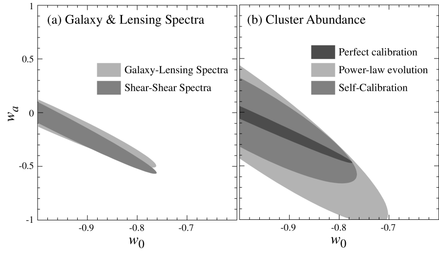
Figure 5.: Dark energy constraints from (a) galaxy and lensing spectra (b) cluster abundance. 10 galaxy bins of $\Delta z=0.1$ out to $z=1$ and 4 shear bins of $\Delta z=0.25$ out to $z=1$ plus a $z\geq 1$ bin with shear noise corresponding to $\bar{n}=10$ gal arcmin^-2 and $\gamma_{\rm rms}=0.16$. Galaxy-galaxy and galaxy-shear power spectra constraints from $50\leq\ell\leq 1000$ are compared with shear-shear spectra from $50\leq\ell\leq 3000$. The cluster abundance is divided into the same bins as the galaxies for $M>10^{14.2}h^{-1}M_{\odot}$ with a comparison between perfect mass calibration, marginalization over a power law mass-observable relation, and self-calibration through employing the sample variance as a measure of the mass dependent clustering of clusters.

Galaxy-lens constraints on the dark energy require the assumption of a model for the association of galaxies to the dark matter whose validity must be verified. Shear-shear correlation on the other hand depend only on the large-scale matter distribution and is theoretically more robust but observationally more difficult to measure. Constraints from the cross correlation of the shear-shear measurements from the same binning scheme and noise assumptions as above are shown in Fig. 5 (Hu 1999). Here we have taken $50\leq\ell\leq 3000$ since the shear field remains Gaussian and theoretically predictable to smaller scales than the galaxy field. Shear-shear and galaxy-lens data of this quality have similar constraining power with regards to the dark energy and may be used to cross-check each other.

Finally let us consider the cluster abundance. The cluster abundance at a fixed mass is exponentially sensitive to the amplitude of linear fluctuations at a given redshift (see e.g. Haiman et al. 2001). Given the CMB normalization of fluctuations at high redshift even the local cluster abundance becomes a constraint on the dark energy that can measure a constant equation of state (see Fig. 3a). At high redshift, the cluster abundance can measure the evolution of the equation of state (Weller et al. 2001). The central concern is whether the cluster selection can be calibrated in mass at the required level of accuracy of better than a few percent. The main hope is that the wealth of observables beyond the optical, extending from the radio to X-ray frequencies, will allow an accurate mass calibration. Given that the full suite will only be available at fairly low redshift, it may be wiser to focus on the mass calibration of the local sample when measuring $w_{\rm DE}$ (Kunz et al. 2003). Recall also that the total growth to $z=0$ is also a good way to separate curvature and dark energy effects.

Nonetheless, let us suppose that we can count all of the clusters above $M_{\rm th}=10^{14.2}h^{-1}M_{\odot}$ in the 10 redshift bins. With a perfect calibration of the mass threshold, the cluster abundance can provide interesting constraints on both $w_{0}$ and $w_{a}$ with the main degeneracy line again following a constant $H_{0}$ (see Fig. 5). If on the other hand, the mass-observable relation that controls the mass threshold $M_{\rm th}$ is allowed to undergo a power law evolution in redshift which must be determined by the abundance measurements themselves, the constraints degrade substantially, especially in the $w_{a}$ direction. Fortunately, clusters have more observables then simply their abundance above threshold in a single observable. With multiple observables it is possible to self-calibrate the mass threshold in principle. Here we show a minimal example of self calibration which involves the sample variance of the cluster counts themselves and hence is fully internal to a cluster abundance survey. Some of the lost information is regained since the sample variance or clustering of clusters as a function of their mass is known from simulations (see Lima & Hu 2004; Majumdar & Mohr 2003 for details).

6. Discussion

The CMB has already provided a set of accurately calibrated standards for dark energy studies. The sound horizon at and distance to recombination is measured to better than 4% and the amplitude of initial fluctuations at large-scale structure scales of $k=0.05$Mpc^-1 to better than 10% by the WMAP data alone. Moreover, the expansion history, e.g. distances, volumes and the Hubble parameter, during the whole deceleration epoch has been determined to the level controlled by errors in $(\Omega_{m}h^{2})^{1/2}$ – currently less than $5\%$ once all of the CMB data is considered. With the high-$z$ expansion history fixed, a measurement of even local $z=0$ observables can determine the dark energy equation of state. The caveat to using this long lever arm to measure the dark energy is that the local and high redshift standards must be accurately calibrated.

CMB inferences are based on an interpretation of the acoustic peaks that has passed internal consistency checks in the damping tail and polarization. The critical assumption underlying the interpretation is the thermal history of the universe and we have focused on recombination and reionization as a challenge for the sub percent level calibration of CMB standards.

Given expected improvements in the measurements of CMB standards, deviations due to the dark energy in distance and growth measures appear mainly at low redshift. The former mainly represent deviations in the Hubble constant. It is ironic that the primary quantity that dark energy probes measure in light of the CMB is the Hubble constant. This includes high-$z$ SNe. Nonetheless, a Hubble constant determination would measure the dark energy equation of state at $z\sim 0.5$ in a flat universe at comparable fractional precision. If this quantity is measured to be inconsistent with a cosmological constant, then distance measures at intermediate redshifts or growth measures at any redshift can be used to test its evolution and/or contamination in its determination from a small spatial curvature. However, in this case the expected deviations are smaller and will require even more accurate measurement and calibration of standards.

CMB standards are naturally exploited by deep optical surveys. The sound horizon appears as baryonic features in angular and spatial power spectra and can be used to measure distances. The density fluctuation calibration enters into the clustering of galaxies, galaxy-galaxy lensing and cosmic shear as well as the abundance of rich clusters. Exploiting these standards with observations that match the accuracy of CMB determinations will be the challenge for future dark energy probes.

Acknowledgments: I thank D. Holz, E. Sheldon and M. White for useful discussions. This work was supported by the DOE and the Packard Foundation and carried out at the KICP under NSF PHY-0114422.

References

- (1)
- (2) Alcock, C., & Paczynski, B., 1979, Nature, 281, 358
- (3) Blake, C., & Glazebrook, K., 2003, ApJ, 594, 665
- (4) Cooray, A., Hu, W., Huterer, D., & Joffre, M., 2001, ApJL, 557, L7
- (5) Eisenstein, D.J., & Hu, W., 1999, ApJ, 511, 5
- (6) Eisenstein, D.J., Hu, W., & Tegmark, M., 1998a, ApJL, 504, L57
- (7) Eisenstein, D.J., Hu, W., & Tegmark, M., 1999b, ApJ, 518, 2
- (8) Frieman, J.A., Huterer, D., Linder, E.V., & Turner, M.S., 2003, Phys.Rev.D, 67, 083505
- (9) Guzik, J., & Seljak, U., 2002, MNRAS, 335, 311
- (10) Haiman, Z., Mohr, J.J., & Holder, G.P., 2001, ApJ, 553, 545
- (11) Hu, W., 1999, ApJL, 522, 21
- (12) Hu, W., 2002, Phys.Rev.D, 65, 023003
- (13) Hu, W., Eisenstein, D.J., Tegmark, M., & White, M., 1999, Phys.Rev.D, 59, 023512
- (14) Hu, W., Fukugita, M., Zaldarriaga, M., & Tegmark, M., 2001, ApJ, 549, 669
- (15) Hu, W., & Haiman, Z., 2003, Phys.Rev.D, 68, 063004
- (16) Hu, W., & Jain, B., 2003, Phys.Rev.D, in press, astro-ph/0312395
- (17) Hu, W., & White, M., 1997, ApJ, 479, 568
- (18) Kaplinghat, M., Knox, L., & Song, Y.S., 2003, Phys.Rev.Lett, 91, 241301
- (19) Kaplinghat, M., Scherrer, R.J., & Turner, M.S., 1999, Phys.Rev.D, 60, 023516
- (20) Kunz, M., Corasaniti, P.S., Parkinson, D., & Copeland, E.J., 2004, Phys.Rev.D, in press, astro-ph/0307346
- (21) Lima, M., & Hu, W., 2004, Phys.Rev.D, in press, astro-ph/0401559
- (22) Linder, E.V., 2003, Phys.Rev.Lett, 90, 130
- (23) Majumdar, M., & Mohr, J.J., 2003, ApJ, submitted, astro-ph/0305341
- (24) Page, L., et al. 2003, ApJS, 148, 233
- (25) Peebles, P.J.E., 1968, ApJ, 153, 1
- (26) Peebles, P.J.E., Seager, S., & Hu, W., 2000, ApJL, 539, L1
- (27) Seager, S., Sasselov, D.D., & Scott, D., 1999, ApJ, 523, 1
- (28) Seljak, U., Sugiyama, N., White, M., & Zaldarriaga, M., 2003, Phys.Rev.D, 68, 083507
- (29) Seo, H.J., & Eisenstein, D.J., 2003, ApJ, 598, 720
- (30) Spergel, D.N., et al. 2003, ApJS, 148, 175
- (31) Spergel, D.N., & Starkman, G., 2002, preprint, astro-ph, 0204089
- (32) Weller, J., Battye, R., & Kneissl, R., 2001, Phys.Rev.Lett, 88, 231301