Assessing the galaxy population out to z$\sim$2

In this work we use the Hubble Deep Field South (HDF-S) version 2 images to assess the galaxy population out to $z\sim 2$. We have used two methods of templates fitting of the spectral energy distributions to obtain photometric redshifts and classify the objects. The Bayesian photometric redshifts gave better results when compared with 54 spectroscopic redshifts available in the literature. Analysis of the rest-frame colour distribution shows a bimodality out to $z\sim 1.4$. We separated our sample in a blue and a red population at $B-V=0.29$. At low redshifts (0.2$<$z$<$0.6), $\sim$60% of the galaxies have $B-V>0.29$ whereas at higher redshifts $\sim$60% of the galaxies are bluer than $B-V<0.29$. Although in low numbers, a population of early-type galaxies (or heavily obscured low redshift galaxies) is seen out to $z\sim$2.

1 Introduction

In spite of the observational and theoretical efforts which have been made since Hubble (1926) classified galaxies according to their morphology, the epoch in which the Hubble types assembled and the process of formation are still unknown. Linking the high-$z$ population with the local universe is one of the most difficult tasks in astronomy. The theoretical predictions such as mass and size evolution are not easily accessible remaining a challenge for the current instruments. Recently, Ravindranath et al. (2004) using the HST/ACS GOODS (Great Observatories Origins Deep Survey done with the Advanced Camera for Surveys with the Hubble Space Telescope) images found no evidence of size evolution of disk galaxies over the redshift range 0.25$<z<$1.25. They find that the number densities of disk galaxies remains fairly constant over this redshift range. Bell et al. (2004) using the COMBO-17 survey (Classifying Objects by Medium-Band Observations in 17 filters) found an increase in stellar mass on the red galaxies (i.e. early-types) by a factor of two since z$\sim$1. These results set strong constraints in the galaxy formation theories such as the hierarchical scenario and the monolithic collapse. In the hierarchical scenario stars are formed continuously over a wide range of redshifts and galaxies are assembled via many generations of mergers of smaller subunits (e.g. White & Frenk 1991, Kauffmann et al. 1993 ). The monolithic collapse theory, on the other hand, predicts rapid star formation at very high redshift ($z>$ 2) followed by a steep decline in the star formation rates (Eggen et al. 1962, Jimenez et al. 1998). If Ravindranath et al. (2004) results are confirmed, disks were already assembled at z$\sim$1.25 and mergers occuring after that epoch would not affect their sizes. Whereas if Bell et al. (2004) results are confirmed, early-type galaxies would have half of their today’s masses at that epoch. Other independent analyses are needed in order to confirm these results.

In this work we use the Hubble Deep Field South (HDF-S) images which has the depth and resolution required to evaluate the galaxy population out to $z\sim$2. The population at higher redshifts has been addressed in the recent studies by Trujillo et al. (2004) and Labbé et al. (2003) using near-infrared observations of the HDF-S where they find a low number of massive galaxies at z$\sim$3, i.e. 1.2 Gyr before the cosmic epoch which we are analyzing in this paper.

In Section 2 we describe the data, photometric redshifts and $K$-corrections, in Section 3 we present the analysis of the rest-frame colour distribution. Conclusions are presented in Section 4.

2 The data

The HDF-S is the second deep field taken with HST (Williams et al. 2000) reaching limiting magnitudes at the 10$\sigma$-level of 26.98, 27.78, 28.34, 27.72 for F300W, F450W, F606W and F814W ($U$, $B$, $V$ and $I$ bands), respectively (Casertano et al. 2000). The WFPC2 field is 163${}^{\prime\prime}\times 183^{\prime\prime}$ or 4.38 arcmin², covered by $4096\times 4600$ pixels.

We have obtained the public version 2 of the WFPC2 HDF-S mosaicked images from the Space Telescope Science Institute’s archive. The version 2 of the HDF-S is an improvement of the first release since the sky background was flattened, a new correction for scattered light in the U-band and more images were added. The noise level decreased and the sky is more homogeneous than in the first version.

The calibration of the raw data is described in Casertano et al. (2000). The four cameras of the WFPC2 were mosaicked into one image, after having been improved by dithering and drizzling. They were also resampled to the same pixel scale (0.0398 arcsec/pixel). The drizzling procedure combines various pointings, preserves photometry and resolution, and removes effects of geometrical distortion.

The image depth fades towards the edges due to the variety of pointings, i.e. the coverage in the edges is lower than in the middle of the separate parts of the image. This means that the outer regions are less reliable, as well as the regions around the cross that separates the four parts of the image. The same was reported by Volonteri et al. (2000a) using the shallower version 1 data.

2.1 Catalogues: Parameters and detections

We have catalogued the objects in the HDF-S using Source Extractor by Bertin & Arnouts (1996; hereafter SE). SE is especially useful for large images with a considerable amount of faint objects. The output from SE is a catalogue of detections including photometry, as chosen by a set of input parameters. The configuration file for SE has many input parameters which were tuned by visual inspection to fit this set of data. Table 1 lists some of the parameters chosen.

I-band Detection		V-band Detection
detect_minarea	18	satur_level	16
detect_thresh	1.4	mag_zeropoint	23.02
deblend_mincount	0.009	gain	680400
clean_param	0.7	pixel_scale	0.0398

Table 1: Source Extractor parameters used. The right half shows values for detection in the $I$-band and the left half values for the photometry in the $V$-band.

We were able to detect objects in the limiting magnitudes of the HDF-S, however there were still some disagreement between over-merging and dividing of spirals. Since no single set of parameters gives a completely satisfactory result, another detection method was used with a larger deblending value. The objects which needed to be altered were visually chosen and manually exchanged.

The catalogue SE produced consists of 1310 detections. After the cleaning process and removing starlike objects, the final catalogue consists of 1142 objects. The magnitudes obtained are AB magnitudes, determined by the zero-point taken from Casertano et al. (2000). We have also used a magnitude-limited sample ($I<26.5$) in the analysis, removing weak detections which yield bad photometric redshifts. The magnitude-limited sample has 591 objects.

In order to avoid different numbers of detections in different filters, we used the dual mode in SE. With the dual mode the same input parameters, such as apertures and positions, were used and the catalogues were matched afterwards. In this case, we decided to use the high S/N $I$-band for detections. Four runs of SE were executed - first a single mode run where both detection and photometry were performed on the $I$-band. Then the parameters for the photometry were changed for each of the other three bands, to obtain the catalogues for the $U$-, $B$- and $V$-bands, respectively.

Another advantage of using the dual mode feature is that the photometry is measured in the same aperture in every band, which is necessary for the photometric redshift determination.

2.2 Photometric redshifts, K-corrections

Photometric redshifts were calculated using methods that fit spectral energy distributions (SED) with templates. We examined two public codes, Hyperz by Bolzonella et al. (2000) and Bayesian Photometric Redshifts (BPZ) by Benitez (2000). A template fitting method compares templates at different redshifts with the four observed datapoints for each object. The best matching spectrum gives both the photometric redshift as well as the galaxy’s spectral type.

The difference between BPZ and standard Maximum Likelihood methods like Hyperz lies in the addition of Bayesian probabilities, and the use of a prior for calculating them. The prior is the central part of the BPZ method. The prior used for this work is the one available in the public code, derived from the HDF-N, and the $I$-magnitude is used as input for the prior determination (base magnitude M_0).

We used four spectral type templates (Coleman, Wu & Weedman 1980) for early-type, Sbc, Scd and irregular galaxies, as well as two blue starburst galaxy templates from Kinney et al. (1996) (SB3 and SB2, the first with a mean colour excess $E(B-V)$ between 0.25 and 0.35, the latter with $E(B-V)$ between 0.11 and 0.21). The spectra are extended to the ultraviolet using a linear extrapolation and a cutoff at 912Å, and to the near infrared using GISSEL synthetic templates. They are corrected for intergalactic absorption following Madau (1995).

Deciding which photometric redshift approach is the best one is not a simple task since the number of spectroscopically confirmed galaxies in the HDF-S only reaches 54 so far (Cristiani et al. 2000, Franceschini et al. 2003, Sawicki & Mallen-Ornellas 2003). In both softwares, the best result is given when using the low-redshift empirical library of SEDs instead of a synthetical template set that takes galaxy evolution into account.

In some cases the spectrum of a galaxy has no good equivalent in the template library, but will still be assigned a redshift corresponding to the closest match, even though it might be far from the observed colours and thus the real redshift. Why then not extend the template library to include more templates, to cover all possible galaxy types? The reason is that the method considers all the templates equal in status, which means that a larger template set increases the number of colour/redshift degeneracies (Benitez, 2000).

In Fig. 1 we compare our Hyperz and BPZ photometric redshifts with three others that are available in the literature: (Stony Brook, Gwyn and Rome (Volonteri et al., 2000b). Since the catalogues were generated with different SE input parameters, we matched the catalogues and considered only the objects in common. Overall our BPZ photometric redshifts agree better with the ones obtained by other groups and thus became our choice for further analysis. The major disagreement is in the upper-left part of the plots, where our values of photometric redshifts are much lower than the ones by the other authors. We have checked those objects and found that they are mostly very faint objects close to the detection limit which will be filtered out in a magnitude-limited sample. Moreover, Benitez (2000) has tested BPZ using the HDF-N which has $\sim 200$ spectroscopic redshifts available with good results, which encouraged us to use his method. Recently, Mobasher et al. (2004a) have also used this method for the GOODS survey which has a larger number of spectroscopically confirmed galaxies in the HDF-N and Chandra Deep Field South.

Fig. 2 shows the photometric redshift distribution of the magnitude-limited catalogue (I$<$26.5) where the majority of objects are found at z$<$2. Unfortunately, the number of spectroscopically confirmed redshifts in the HDF-S is not as high as in the HDF-N. We found 54 redshifts within the WFPC2 area we are using. Sawicki & Mallen-Ornellas (2003) have 55 spectroscopic redshifts, but six of these are double detections (i.e. the resolution of the ground-based observations was not good enough, making two galaxies share the same redshift) and three are not within the boundaries of the WFPC2 area we are using. Fig. 3 shows the comparison between our BPZ photometric redshifts and the spectroscopic redshifts. We concluded that our photometric redshifts are overall in good agreeement with the spectroscopic redshifts. However, there are very few objects with spectroscopic redshifts $z>1.5$ available in the literature. We will limit our analysis to the range 0.2$<z<$1.4 where we have enough spectroscopic redshifts to test the photometric redshifts. There are seven objects with photometric redshifts significantly different from their spectroscopic redshifts (Table 2). We note that all but one of the discordant redshift objects were assigned an early-type template. We believe that wrong redshifts were assigned due to extinction corrections which were not applied in our spectral classification. Taking into consideration that we only had 4 colours, the template fitting method to obtain redshifts worked remarkably well. This is an important result considering how time consuming deep $HST$ observations are.

Id	$Phot-z$	$Spect-z$	Type	IAB	$B-V$
306	0.13	0.7342	1	20.0	0.7041
594	1.96	0.5648	2	23.0	0.4517
638	1.89	0.5817	2	23.0	0.4794
1091	1.56	0.7594	2	23.8	0.4871
1264	1.73	0.6963	2	25.0	0.4805
632	0.71	1.27	2	22.9	0.4319
1101	1.66	0.1148	4	23.8	0.2460

Table 2: Catalogue number, BPZ photometric redshift, spectroscopic redshift, spectral type (1=E, S0, Sa, 2=Sbc), I_AB magnitude, $B-V$ colour.

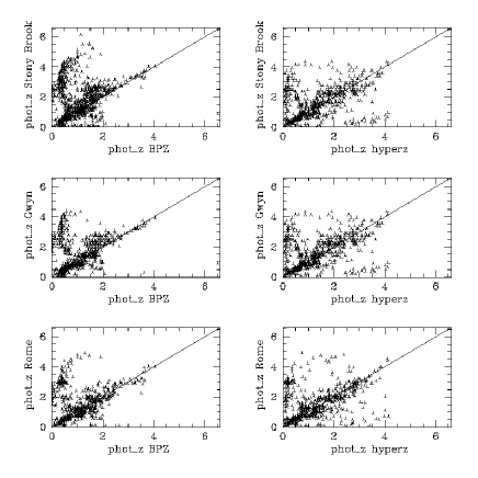
Figure 1: Comparison between our photometric redshifts obtained with Hyperz and BPZ with other catalogues: the Stony Brook group, Gwyn and the Rome group Volonteri (2000b).

Figure 2: Distribution of BPZ photometric redshifts of the magnitude-limited catalogue ($I<26.5$).

Figure 3: Comparison between photometric redshifts and spectroscopic redshifts.

The rest-frame magnitudes were calculated using $K$-corrections and distance moduli provided by T. Dahlén (2003, priv. comm.), covering redshifts up to $z=7$ for the six spectral types and a cosmology with $H_{0}=70$ km s^-1Mpc^-1, $\Omega_{M}=0.3$ and $\Omega_{\Lambda}=0.7$.

2.3 Spectral types

Since the first Hubble Deep Field images (Williams et al. 1996) several authors have attempted to classify the morphology of faint galaxies (e.g. Abraham et al. 1996, van den Bergh et al. 1996, Corbin et al. 2001, Menanteau et al. 2001, van den Bergh et al. 2002). Automatized methods of classification, such as the one which measures structural parameters (e.g. Conselice 2003), produce valuable results (e.g. Conselice et al. 2004, Mobasher et al. 2004b). However, instead of using the concentration of stellar light and its asymmetric distribution to classify the galaxies in the HDF-S we chose to use the spectral types which were obtained from the template fitting in the photometric redshift technique as a morphology indicator. This latter method keeps the classification directly attached to the photometric redshift estimates. Moreover, the spectral types are associated with the spectral energy distribution which reflects the physical properties of the objects, such as star formation history. We have randomly selected a sub-sample (15% of the total sample) for visual inspection. A gallery of typical galaxies is available online. The gallery is divided in spectral types and redshift bins. Galaxies with 0.2$<z<$1 which were assigned an E-Sa spectral template indeed resemble classical early-type galaxies whereas more distant galaxies (1$<z<$2) are red objects too faint to be visually classified. Galaxies which were assigned Sbc and Scd spectral templates show the presence of a disk in the low redshift bins and star formation. The ones assigned irregular and starburst (SB2 and SB3) templates have clearly peculiar morphologies in all redshifts. Some SB3 galaxies with 0.2$<z<$0.5 are less peculiar showing disks with strong knots of star formation. We have not attempted to correct for extinction and we are aware of the effects that this can cause. For instance, the red colours in the early type galaxies at high$-z$ might be due to dust and not due to an old population. However, considering the good agreement that we have obtained in the photometric redshifts, only a few objects would require strong extinction correction which would change the spectral type assigned.

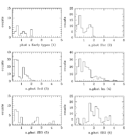
Figure 4: Distribution of BPZ photometric redshifts for each of the galaxy types.

The redshift distribution for each spectral type (Fig. 4) clearly shows that the number of early-type galaxies (E, S0, Sba) decreases with redshift. The amount of irregular and starburst galaxies, on the other hand, increases with redshift. There is a high amount of irregulars all through the redshift range covered. However, at high redshifts, only irregulars and starbursts are present. The irregulars peak at $0.75<z<1.0$, and starbursts (SB2) at $z>1.0$. This is in agreement with Volonteri et al. (2000b) who found that early-type galaxies show a steep decrease in number counts in the faintest bin.

			Red Group				Blue Group
catalogues	mean	$\sigma$	median	objects	mean	$\sigma$	median	objects
$a$	0.458	0.247	0.400	440	0.125	0.119	0.161	700
$b$	0.429	0.138	0.385	317	0.166	0.095	0.186	274
$c$	0.440	0.131	0.404	257	0.153	0.087	0.170	334
$d$	0.424	0.128	0.379	174	0.194	0.057	0.197	123
$d2$	0.399	0.065	0.405	107

Table 3: Mean, $\sigma$ and median values of the $B-V$ colours listed for the full catalogue and its subsamples. $a$ is the full catalogue, $b$ is the magnitude-limited catalogue, $c$ is the full catalogue limited in redshift ($0.2<z<1.2$) and $d$ is the magnitude-limited catalogue limited in redshift. $d_{2}$ is the red group from $d$ without the red objects.

3 Discussion

The colour distribution for all galaxies in the sample and for the magnitude-limited sample is shown in Fig. 5. For comparison, local late-types (Scd) and irregular galaxies have $B-V$=0.15–0.48 ($B-V$=0.27–0.60 Johnson filters), whereas earlier types have $B-V=$0.73–0.80 (B-V=0.85–0.92) (Liu & Green 1998). Therefore, we are clearly detecting a larger number of star-forming galaxies in all redshift bins. Two distinct populations of objects are clearly seen in Fig. 5, one which is redder than $B-V=0.29$, and one which is bluer than that. The bimodality in the colour distribution of galaxies has recently been seen by Strateva et al. (2001) using the Sloan Digital Sky Survey, Hogg et al. (2002) for the local universe ($z<0.22$) and Bell et al. (2004) out to $z\sim 1$. For our sample, the bimodality is actually still visible out to a redshift of $z\sim 1.4$. Similar analysis using the ESO Imaging Survey (EIS) has shown a bimodality for redshifts out to $z\sim 1.6$ for a much larger area in the sky (J. Andersson private communication). The colours of galaxies reflect their star formation history, therefore a bimodality in colours suggests that they have gone through different evolutionary paths.

Figure 5: Colour distribution for all galaxies in the sample and for the magnitude-limited sample.

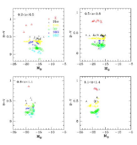
Figure 6: Rest-frame colour-magnitude diagram for four redshift bins.

We chose to do the analysis on the magnitude-limited sample ($I<26.5$) instead of the entire catalogue which has limiting I-magnitude 28.6. The disadvantage in using the former sample is the smaller number of objects. However, the latter sample would include spurious faint outliers which were still present in the redshift-limited catalogue. A consequence of this limitation is that objects are being dropped from the sample. The colour-magnitude diagrams are shown in Fig. 6. Comparing Fig. 6 with Fig. 4 we notice that there are many more starbursts and irregulars in the entire sample than in the magnitude-limited sample.

In Table 3 we give the average mean, $\sigma$ and median of the $B-V$ colours for the blue and red sample using the full catalogue and the magnitude-limited catalogue. We also include the same for the redshift-limited catalogue. The average colour of the blue catalogue is $B-V=0.125\pm 0.119$, whereas the mean value for the magnitude and redshift-limited sample is $B-V=0.194\pm 0.057$ showing a low dispersion in colours. The average colour of the red catalogue is strongly affected by a small group of redder objects with $B-V>0.7$ present in the top of the plots, which is still noticeable in the highest redshift bin of Fig. 6. The red group has a larger standard deviation ($\sigma$) than the blue, caused by these redder objects. If we remove them from the red sample (d2 in Table 3), the dispersion in the colour is comparable with the one for the blue group. The red group is on average a factor of 2 redder than the blue group (sample d in Table 3). For comparison, the u^∗–r^∗ colours of the red group in Strateva et al. (2001) is also $\sim$ 2 times redder than the blue group (from Fig. 2 in their paper) while in Bell et al. (2004) the $U-V$ colours of the red population can be as high as three times the colours of the blue population (From Fig. 1 in their paper). We find a factor of $\sim 3$ (or higher) if we use the reddest objects instead of average values. However, there are very few of these red objects and a larger field is needed to improve the statistiscs.

The median redshift for the blue population is $z$=0.65 whereas for the red population is $z$=0.57. One interesting result is the fact that the redder objects have median $z$=0.61 and the bluer objects have $z$=$0.3-0.4$. These red objects probably have an older stellar population and/or are heavily extinct, whereas the blue ones are galaxies experiencing star formation. There are also a few very blue objects with $B-V<0.1$. These are strong starburst galaxies at low redshifts with $B-V$ bluer than local irregular galaxies.

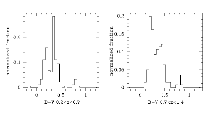
Figure 7: Histograms of the magnitude-limited catalogue, divided into two redshift bins.

The bimodality of colours is seen at low and high redshifts (Fig. 7). In the first bin, at lower redshifts, $\sim$60% of the galaxies have ($B-V>0.29$) whereas at higher redshifts $\sim$60% of the galaxies are bluer than $B-V<0.29$. The increase in blue galaxies at higher redshifts is clearly due to the irregulars and starbursts as shown in Fig. 6. We can also see in Fig. 6 that the starburst galaxies of type SB2 are generally bluer than the irregular galaxies and are also contributing to the blue colors. The starbursts SB3, on the other hand, are redder and not all of them have $B-V<0.29$.

Although in lower numbers ($\sim$5%) than late-type galaxies, early-type galaxies are also seen out to z$\sim$2. This has important implications in galaxy evolution since it might imply that early-type galaxies are already in place at z$>$1. The question of when these galaxies are assembled will soon be answered when larger deep fields in multiwavelengths will be analysed. A caveat to be considered is the role of dust in galaxy evolution. Galaxies with large amount of dust such as submm galaxies (e.g. Eales et al. 2000) and $K$-luminous galaxies (Daddi et al. 2004) would not be easily detected in the images due to extinction and in case they were detected they would be too faint and lower than the magnitude limit adopted. However, we cannot exclude the possibility that these redder galaxies are being heavily obscured by dust. Combining UV-optical with infrared is then essential (Conselice et al. 2003). Soon deep infrared images, such as the recent NICMOS Ultra Deep Field images, and future Spitzer images combined with HST UV-optical will be ideal for the study of galaxy evolution.

4 Summary

We have analysed the HDF-S $U,B,V,I$ images in order to assess the galaxy population at $z<2$. We summarize our main results as follows:

1. The template fitting method, BPZ, gives better photometric redshifts than other redshift estimates and agrees well with the 54 spectroscopic redshifts available in the literature. Some disagreement persisted for faint objects close to the detection limit, and this conducted us to produce and perform the analysis on a magnitude-limited catalogue of 591 objects with $I<26.5$.

2. The spectral types obtained from the template fitting were used as morphological indicator. The quality of the automated spectral type assignments was carefully checked by visual inspection. A gallery with typical types was produced.

3. A bimodal distribution of $B-V$ colours was found out to $z\sim 1.4$. At low redshifts (0.2$<$z$<$0.6), $\sim$60% of the galaxies have ($B-V>0.29$) whereas at higher redshifts $\sim$60% of the galaxies are bluer than $B-V<0.29$. The blue population has $<B-V>=0.194\pm 0.057$ and the red population has $<B-V>=0.399\pm 0.065$. There is also a group of red objects with $B-V>0.7$ present in all redshift bins whereas the bluest objects with $B-V<0.2$ are seen only in the lowest redshift bins ($0.2<z<0.5$).

4. Galaxies with spectral types typical or irregulars and starbursts are more numerous at higher redshifts ($z>0.8$) than Sbc, Scd and early-types.

5. The redder objects have median $z$=0.61 whereas the bluer objects have $z$=$0.3-0.4$.

6. Although in lower numbers (5%), a population of early-type galaxies (or heavily obscured low redshift galaxies) is seen out to $z\sim$2.

The results presented here suggest that galaxies of all spectral types (E-Sa, Sbc, Scd, Irr and starbursts) are seen out to $z\sim 1.4$ and are separated in a blue and a red population. This bimodality in colours suggest that galaxies have different star formation histories which could lead to the different Hubble types seen in the local universe. Multiwavelength deep observations of large areas are needed in order to establish the epoch of galaxy formation.

- (1) Abraham, R.G., Tanvir, N.R., Santiago, B.X., Ellis, R.S., Glazebrook, K.G., van den Bergh, S. 1996, MNRAS, 279, 47
- (2) Andersson, J., de Mello, D.F., & Rydbeck, G. 2004, in preparation
- (3) Benitez, N. 2000, ApJ, 536, 571
- (4) Bertin, E., & Arnouts, S. 1996, A&AS, 117, 393
- (5) Bell, E., Wolf,C., Meisenheimer, K., Rix, H-W, Borch, A., et al. 2004, ApJ, 608, 752
- (6) Bolzonella, M., Miralles, J.-M., Pello, R. 2000, A&A, 363, 476
- (7) Casertano, S., et al. 2000, AJ, 120, 2747
- (8) Coleman, G.D., Wu, C-C., & Wedman, D.W. 1980, ApJS, 43, 393
- (9) Conselice, C.J. 2003, ApJS, 147, 1
- (10) Conselice, C.J., Bershady, M.A., Dickinson, M., & Papovich, C. 2003, AJ, 126, 1183
- (11) Conselice, C.J. et al. ApJ, 2004, 600, L139
- (12) Corbin, M. et al., 2001, ApJ, 551, 23
- (13) Cristiani, S. et al., 2000, A&A, 359, 489
- (14) Daddi et al. 2004, ApJ, 600, L127
- (15) Eggen, O.J., Lynden-Bell, D., & Sandage, A.R. 1962, ApJ, 136, 748
- (16) Eales, S., et al. 2000, AJ, 120, 2244
- (17) Franceschini, A., et al. 2003, A&A, 403, 501
- Hogg et al. (2002) Hogg, D. W., et al. 2002, AJ, 124, 646
- (19) Jimenez et al. 1999, MNRAS, 305, 16
- (20) Kauffmann, G., White, S.D.M., Guiderdoni, B. 1993, MNRAS, 264, 201
- (21) Kinney, A. et al. 1996, ApJ, 467, 38
- (22) Labbé et al. 2003, AJ, 125, 1107
- (23) Liu, C.T.,& Green, R.F. 1998, ApJ, 116, 1074
- (24) Madau, P. 1995, ApJ, 441, 18
- (25) Menanteau, F., Abraham, R.G., & Ellis, R.S. 2001, MNRAS, 322, 1
- (26) Mobasher, B., et al. 2004a, ApJ, 600, L167
- (27) Mobasher, B., et al. 2004b, ApJ, 600, L143
- (28) Ravindranath, S., et al. 2004, ApJ, 604, L9
- (29) Sawicki, M., & Mallen-Ornelas, G. 2003, AJ, 126, 1208
- Strateva et al. (2001) Strateva, I., et al. 2001, AJ, 122, 1861
- (31) van den Bergh, S., Abraham, R.G., Ellis, R.S., Tanvir, N.R., Santiago, B.X., Glazebrook, K.G. 1996, AJ, 112, 359
- (32) van den Bergh, S., Abraham, R.G., Whyte, L.F., Merrifield, M.R., Eskridge, P.B., Frogel, J.A., Pogge, R. 2002, AJ, 123, 2913
- (33) Volonteri, M., Saracco, P., & Chincarini, G. 2000a, A&AS, 145, 111
- (34) Volonteri, M., Saracco, P., Chincarini, G., & Bolzonella, M. 2000b, A&A, 487, 500
- (35) White, S.D.M., Frenk, C.S. 1991, ApJ, 379, 52
- (36) Williams, R.E., et al. 2000, AJ, 120, 2735
- (37) Williams, R.E., et al. 1996, AJ, 112, 1335