Self-Consistent Theory of Halo Mergers

Abstract

The rate of merging of dark-matter halos is an absolutely essential ingredient for studies of both structure and galaxy formation. Remarkably, however, our quantitative understanding of the halo merger rate is still quite limited, and current analytic descriptions based upon the extended Press-Schechter formalism are fundamentally flawed. We show that a mathematically self-consistent merger rate must be consistent with the evolution of the halo abundance in the following sense: The merger rate must, when inserted into the Smoluchowski coagulation equation, yield the correct evolution of the halo abundance. We then describe a numerical technique to find merger rates that are consistent with this evolution. We present results from a preliminary study in which we find merger rates that reproduce the evolution of the halo abundance according to Press-Schechter for power-law power spectra. We discuss the limitations of the current approach and outline the questions that must still be answered before we have a fully consistent and correct theory of halo merger rates.

1 Introduction

In current cosmological theory the mass density of the Universe is dominated by dark matter. The most successful model of structure formation is that based upon the concept of cold dark matter (CDM). In the CDM hypothesis dark-matter particles interact only via the gravitational force. Since the initial distribution of density perturbations in these models has greatest power on small scales, the first objects to collapse and form dark-matter halos are of low mass. Larger objects form through the merging of these smaller sub-units. Consequently, the entire process of galaxy formation is thought to proceed in a “bottom-up”, hierarchical manner.

Clearly then, the rate of dark-matter–halo mergers is an absolutely crucial ingredient in models of galaxy and large-scale-structure formation, from sub-galactic scales to galactic and galaxy-cluster scales. The Press-Schechter (PS) formalism (?) has long provided a simple, intuitive, and surprisingly accurate formula for the distribution of halo masses at a given redshift over a large range of mass scales and for a vast variety of initial power spectra. This formalism states that the number of halos per comoving volume with masses in the range $M\rightarrow M+{\rm d}M$ is (?)

$$n(M;t){\rm d}M = \sqrt{2\over\pi}{\rho_{0}\over M^{2}}{\delta_{c}(t)\over\sigma(M)}\left|{{\rm d}\ln\sigma\over{\rm d}\ln M}\right|$$ (1)

$$\times\exp\left[-{\delta_{c}^{2}(t)\over 2\sigma^{2}(M)}\right]{\rm d}M,$$

where $\rho_{0}$ is the background density and $\delta_{\rm c}(t)$ is the critical overdensity for collapse in the spherical-collapse model. Here, $\sigma(M)$ is the root variance of the primordial density field in spheres containing mass $M$ on average, extrapolated to $z=0$ using linear theory; it can be determined from the primordial power spectrum $P(k)$ that is specified by inflation-inspired models for primordial perturbations. For power-law power spectra, $P(k)\propto k^{n}$ and $\sigma(M)\propto M^{-(3+n)/6}$; in this case, the Press-Schechter halo abundance diverges as $n(M)\propto M^{(-9+n)/6}$ as $M\rightarrow 0$, and it is exponentially suppressed above a characteristic mass $M_{*}(t)$ determined from the condition $\delta_{c}(t)=\sigma(M_{*})$. The critical overdensity $\delta_{c}(t)$ is a monotonically decreasing function of $t$ so that the Press-Schechter distribution shifts to larger masses with time, i.e. $\dot{M}_{*}>0$. The fraction of cosmological mass in halos of mass $M\rightarrow M+{\rm d}M$ is $Mn(M){\rm d}M/\rho_{0}$, and, at any given time, most of the mass resides in halos with masses $M\sim M_{*}$. Note that although the number of halos diverges as $M\rightarrow 0$, the total mass in halos remains finite.

An elegant paper by ?—and similar work by ? and ?—extended the work of Press and Schechter to determine the rate at which halos of a given mass merge with halos of some other mass. In addition to providing valuable physical insight, these merger rates have extraordinary practical value, having been applied to galaxy-formation models, e.g., if galaxy morphologies are determined by the merger history (?); AGN activity (?); models for Lyman-break galaxies (?); abundances of binary supermassive black holes (SMBHs) (?); rates for SMBH coalescence (?) and the resulting LISA event rate (?; ?); the first stars (?; ?); galactic-halo substructure (?; ?; ?; ?; ?); halo angular momenta (?) and concentrations (?); galaxy clustering (?); particle acceleration in clusters (?); and formation-redshift distributions for galaxies and clusters and thus their distributions in size, temperature, luminosity, mass, and velocity (?; ?).

Amazingly enough, however, these merger rates are fundamentally flawed. As we show below, the extended-Press-Schechter (EPS) formulae for merger rates are mathematically self-inconsistent, providing two different results for the same merger rate. The two different merger rates are plotted in Fig. 1. They are equal for equal-mass mergers but increasingly discrepant for larger mass ratios. This ambiguity will be particularly important for, e.g., understanding galactic substructure and for SMBH-merger rates. Even the smaller numerical inconsistency for mergers of nearly equal mass may be exponentially enhanced during repeated application of the formula while constructing merger trees to high redshift. Moreover, the ambiguity calls into question the entire formalism, even when the two possibilities seem to give similar answers quantitatively.

In this paper, we discuss the mathematical requirements of a self-consistent theory of halo mergers. As recognised already (?; ?; ?), the merger process is described by the Smoluchowski coagulation equation. This equation simply says that the rate at which the abundance of halos of a given mass changes is determined by the difference between the rate for creation of such halos by mergers of lower-mass halos and the rate for destruction of such halos by mergers with other halos. The correct expression for the merger rate must be one that yields the correct rate of evolution of the halo abundance when inserted into the coagulation equation The problem is thus to find a merger rate, or “kernel,” that is consistent with the evolution of the halo abundance, either the Press-Schechter abundance or one of its more recent N-body–inspired variants (?; ?).

The apparent simplicity of the mathematical problem, which appears in equation (7) below, is in fact quite deceptive. The Smoluchowski coagulation equation is in fact an infinite set of coupled nonlinear differential equations. The equation appears in a variety of areas of science—e.g., aerosol physics, phase separation in liquid mixtures, polymerization, star-formation theory (?; ?), planetesimals (?; ?; ?), chemical engineering, biology, and population genetics—so there is a vast but untidy literature on the subject (although see ? for an illuminating review). It has been studied a little by pure and applied mathematicians (?). Still, solutions to the coagulation equation are poorly understood. Furthermore, there is virtually no literature on the problem we face: i.e., how to find a merger kernel that, when inserted into the coagulation equation, yields the desired halo mass distribution and its evolution as a solution.

In this paper, we present a numerical technique to find a merger kernel that yields the correct evolution of a specified halo mass distribution. We demonstrate this technique by applying it to Press-Schechter distributions for power-law power spectra. We regret that at this point we still do not have results that can be applied to astrophysical merger rates (e.g. those valid for CDM power spectra), although our techniques can easily be extended to more realistic cases. Moreover, although we have indeed found merger rates that are mathematically consistent with the desired halo distributions, our inversion of the Smoluchowski equation is not necessarily unique. As we discuss below, there may be other merger kernels that also yield the same halo mass distribution. More work must be done to determine how to insure that the numerical inversion yields the merger kernel that in fact describes the process of mergers from gravitational clustering of mass with an initial Gaussian distribution. Nevertheless, the work presented here may be a first step in this direction.

Below, in §2, we first review the extended Press-Schechter calculation and show that it gives mathematically inconsistent expressions for the merger rate. In Section 3, we then discuss the coagulation equation that needs to be solved. Section 4 describes our numerical algorithm for finding self-consistent merger rates. Section 5 and Figs. 2–8 show results of our numerical inversion for a variety of power-law power spectra. Section 6 answers some common questions about this work, and Section 7 provides some concluding remarks and outlines some questions that must still be addressed in future work. Appendix A provides an alternative formulation of the coagulation equation that makes the cancellation of divergences explicit. Appendix B provides, for reference, derivations of the two fo the known analytic solutions to the coagulation equation.

2 Review of the Extended Press-Schechter Calculation

The extended Press-Schechter theory (?; ?; ?; ?) predicts the distribution of masses of progenitor halos for a halo of a given mass. By manipulating the equations of this theory it is possible to obtain an expression for the merger rate of halos of mass $M_{1}$ with those of mass $M_{2}$. ? give the following expression for the probability per unit time that a halo of mass $M_{2}$ will merge with a halo of mass $M_{1}=M_{\rm f}-M_{2}$ to make a halo of mass $M_{\rm f}$

$${{\rm d}^{2}p\over{\rm d}M_{2}{\rm d}t} = {1\over M_{\rm f}}\sqrt{2\over\pi}\left|{\dot{\delta}_{c}\over\delta_{c}}\right|\left|{{\rm d}\ln\sigma(M_{f})\over{\rm d}\ln M_{f}}\right|{\delta_{c}(t)\over\sigma(M_{f})}$$ (2)

$$\times {1\over\left[1-\sigma^{2}(M_{f})/\sigma^{2}(M_{1})\right]^{3/2}}$$

$$\times \exp\left[-{1\over 2}\delta_{c}(t)\left({1\over\sigma^{2}(M_{f})}-{1\over\sigma^{2}(M_{1})}\right)\right].$$

In the extended-Press-Schechter formalism, the abundance of halos of mass $M$ is still given by equation (1). The total number of mergers between halos of mass $M_{2}$ and $M_{1}$ per unit time and per unit volume must therefore be

$$R(M_{1},M_{2};t)=n(M_{2};t){{\rm d}^{2}p\over{\rm d}M_{2}{\rm d}t}.$$ (3)

Since the merger rate is proportional to both $n(M_{1};t)$ and $n(M_{2};t)$ we define a merger kernel $Q(M_{1},M_{2};t)$ (which has units of cross section times velocity) through

$$R(M_{1},M_{2};t)=Q(M_{1},M_{2};t)n(M_{1};t)n(M_{2};t).$$ (4)

From equations (1)–(4) we can derive

$$Q(M_{1},M_{2};t) = {M_{2}^{2}\over\rho_{0}\sigma_{\rm f}}{\sigma_{2}\over M_{2}}\left|{\dot{\delta}_{c}\over\delta_{c}}\right|\left|{{\rm d}\ln\sigma_{f}\over{\rm d}\ln M_{\rm f}}\right|\left|{{\rm d}\ln\sigma_{2}\over{\rm d}\ln M_{2}}\right|^{-1}$$ (5)

$$\times {1\over(1-\sigma_{\rm f}^{2}/\sigma_{1}^{2})^{3/2}}$$

$$\times \exp\left[-{\delta_{c}^{2}\over 2}\left({1\over\sigma_{\rm f}^{2}}-{1\over\sigma_{2}^{2}}-{1\over\sigma_{1}^{2}}\right)\right],$$

where we have adopted the notation $\sigma_{2}=\sigma(M_{2})$, etc. The problem with this merger rate is immediately apparent. Clearly $R(M_{1},M_{2};t)=R(M_{2},M_{1};t)$ must always hold; i.e., the merger rate must be a symmetric function of its arguments. However, this is not the case for the above definition of $Q(M_{1},M_{2};t)$. This can be seen clearly in Fig. 1 where we plot the merger kernels $Q(M_{1},M_{2};t)$ and $Q(M_{2},M_{1};t)$ for a specific case. Although the differences between the two predicted merger rates are small over most of the range of $M_{1}/M_{2}$ plotted, it is important to note that the discrepancies may have significant consequences for cosmological studies. For example, the merger rate for a mass ratio of $10^{-5}$ is uncertain by a factor of $10$. This could significantly affect the predicted number of dwarf galaxies expected to be found within clusters. It is very problematic for predictions of black-hole mergers detectable with LISA, as many of the detectable signals may arise from mergers of very unequal masses for which the numerical ambiguity is particularly pronounced. Furthermore, even for mergers of nearly equal masses, where the two predictions agree more closely, repeated application of the merger-rate formula (as occurs in the construction of merger trees) will lead to a growing divergence between the two predictions.

Figure 1: The dark-matter-halo merger rate computed using the extended Press-Schechter formula of ?. Results are shown for an $n=1$ power-law power spectrum, a halo of mass $M_{1}=10^{12}h^{-1}M_{\odot}$ at $z=0$ in a Universe with $\Omega_{0}=0.3$, $\Lambda_{0}=0.7$, $\sigma_{8}=0.9$ and $\Gamma=0.21$. The two lines show the result of using the two versions of the merger rate predicted by the extended Press-Schechter theory.

The extended-Press-Schechter merger rate is in fact only a symmetric function of its arguments in two special cases. The first, trivial, case is when $M_{1}=M_{2}$. The second is for the case of a distribution of primordial densities described by a white-noise power spectrum, $P(k)\propto k^{n}$ with $n=0$. In this case the merger kernel reduces to

$$Q(M_{1},M_{2};t)={(M_{1}+M_{2})\over\rho_{0}}\left|{\dot{\delta}_{c}\over\delta_{c}}\right|.$$ (6)

Our aim is to find kernels $Q(M_{1},M_{2};t)$ which (a) are symmetric in their arguments and (b) yield the correct evolution of the halo distribution $\dot{n}(M)$ when inserted into the coagulation equation. The kernel should also (c) satisfy the known statistics of dark-matter–halo merger rates. Below, we will illustrate a numerical algorithm that can accomplish conditions (a) and (b); we discuss the third condition later.

3 Basic Equations

During the process of hierarchical clustering, halos of mass $M$ will be created via mergers of pairs of halos of masses $M^{\prime}$ and $M-M^{\prime}$, and they will be destroyed via mergers with halos of any other mass, $M^{\prime}$. The rate at which the abundance of halos of mass $M$ changes is therefore

$$\dot{n}(M)={1\over 2}\int_{0}^{M}n(M^{\prime})n(M-M^{\prime})Q(M^{\prime},M-M^{\prime}){\rm d}M^{\prime}$$

$$-n(M)\int_{0}^{\infty}n(M^{\prime})Q(M,M^{\prime}){\rm d}M^{\prime},$$ (7)

where the dot denotes a derivative with respect to time, the first term on the right-hand side describes halo formation, and the second describes halo destruction. Note that we have suppressed the explicit dependence of $n(M;t)$ on time and the possible dependence of $Q(M_{1},M_{2};t)$ on time in equation (7). This equation is known as the Smoluchowski coagulation equation (?). It appears in a variety of areas in science in which coagulation processes occur. One astrophysical example is the theory of planetesimal growth, in which small objects merge to form larger objects. In almost all prior applications, the merger kernel $Q(M,M^{\prime};t)$ is specified by (micro)physical processes (note that it has units of cross section times velocity) and the equations are then integrated forward from some initial mass distribution $n(M,t=0)$ to determine the mass distribution at some later time.

In our case, however, we know the “answer,” the mass distribution $n(M,t)$ (either a Press-Schechter distribution, an improved version such as the Sheth-Tormen distribution, or some other similar distribution determined from simulations). We need to find the merger kernel $Q(M_{1},M_{2};t)$ that yields the desired evolution of this mass distribution when inserted into the Smoluchowski equation. This, as far as we know, is an unsolved mathematical problem. In principle, some variant of the derivation used by ? that imposes the symmetry constraint $Q(M_{1},M_{2};t)=Q(M_{2},M_{1};t)$ might be used to determine this merger kernel. It is in fact easy to impose the symmetry constraint with some ansatz, such as an arithmetic or geometric mean of the two Lacey–Cole results. However, the merger kernel must also be consistent, within the dictates of the coagulation equation, with the evolution of the Press-Schechter halo distribution, and we have not yet been able to satisfy this constraint with any analytic approach.

In the absence of an analytic solution, we attempt to find a numerical solution to the problem: i.e., can we numerically find a merger kernel $Q(M_{1},M_{2};t)$ that when inserted into the coagulation equation yields the evolution of the PS distribution? The answer, as we discuss below, is yes. To illustrate the technique, we restrict our attention to the Press-Schechter mass distribution because of the simplicity of the analytic expressions. Moreover, we restrict our attention to power-law power spectra, $P(k)\propto k^{n}$, again for simplicity. This has the additional advantage that for the case $n=0$ we have an analytic solution to the Smoluchowski equation. However, our technique can be applied equally well to more accurate distributions such as the Sheth-Tormen distribution and to other power spectra.

The Press-Schechter rate of change of halo abundance is found by differentiating equation (1) and is given by

$$\dot{n}(M_{1},t)=-\sqrt{{2\over\pi}}{\rho_{0}\over M_{1}^{2}}{\delta_{\rm c}\over\sigma_{1}}\alpha\exp\left[-{1\over 2}{\delta_{\rm c}^{2}\over\sigma_{1}^{2}}\right]{\dot{\delta}_{\rm c}\over\delta_{\rm c}}\left[{\delta_{\rm c}^{2}\over\sigma_{1}^{2}}-1\right].$$ (8)

Shifting to a time variable $\tau=-\ln\delta_{\rm c}(t)$ and dimensionless mass variable $z=M/M_{\star}(\tau)$ [where $M_{\star}(\tau)$ is the characteristic nonlinear mass scale defined through the relation $\sigma(M_{\star})=\delta_{\rm c}(\tau)$] this becomes

$${{\rm d}n\over{\rm d}\tau}(z_{1})=\sqrt{{2\over\pi}}{\rho_{0}\over M_{\star}}z_{1}^{-2}{\delta_{\rm c}\over\sigma_{1}}\exp\left[-{1\over 2}{\delta_{\rm c}^{2}\over\sigma_{1}^{2}}\right]\left[{\delta_{\rm c}^{2}\over\sigma_{1}^{2}}-1\right].$$ (9)

where $\alpha=|{\rm d}\ln\sigma/{\rm d}\ln M|=(3+n)/6$. For power-law power spectra, $\sigma(M)=\sigma(M_{\star})z^{-(3+n)/6}=\delta_{\rm c}z^{-(3+n)/6}$. Therefore,

$${{\rm d}n\over{\rm d}\tau} = \sqrt{{2\over\pi}}{\rho_{0}\over M_{\star}}z_{1}^{(-9+n)/6}\alpha$$ (10)

$$\times\exp\left[-{1\over 2}z_{1}^{(3+n)/3}\right]\left[z_{1}^{(3+n)/3}-1\right].$$

The Press-Schechter abundance is simply

$$n(z)=\sqrt{{2\over\pi}}{\rho_{0}\over M_{\star}}z_{1}^{(-9+n)/6}\alpha\exp\left[-{1\over 2}z_{1}^{(3+n)/3}\right].$$ (11)

In these variables, the Smoluchowski equation is

$${{\rm d}n\over{\rm d}\tau}(z) = {1\over 2}\int_{0}^{z}n(z^{\prime})n(z-z^{\prime})q(z^{\prime},z-z^{\prime}){\rm d}z^{\prime}$$ (12)

$$-\int_{0}^{\infty}n(z)n(z^{\prime})q(z,z^{\prime}){\rm d}z^{\prime},$$

where we have used $q$ to denote the merger kernel in our new system of mass and time variables. Our goal is to find $q(z_{1},z_{2};\tau)$. Clearly the solution must be proportional to $\sqrt{\pi/2}M_{\star}(\tau)/\rho_{0}\alpha$. We therefore choose a system of units such that $\sqrt{\pi/2}M_{\star}(\tau)/\rho_{0}\alpha=1$ to simplify the calculation. This choice of units removes the explicit time dependence from our merger rate, allowing us to find a function $q(z_{1},z_{2})$ valid at all times. The time dependence of the merger rate is absorbed into a time-dependent system of units instead.

Before discussing our numerical algorithm, we first point out that, for the mass functions we are considering, there are divergences in the creation and destruction terms in the coagulation equation that cancel. As $z\rightarrow 0$, the mass function $n(z)\propto z^{-\gamma}$, where $\gamma=(9-n)/6$ is between 2 and 1 for $-3<n<3$. Thus, if $q(z_{1},z_{2})$ does not vanish as one of the arguments approaches zero (which is the case for $n=0$, and as we argue below, should also be the case more generally), then there is a non-integrable singularity at the lower and upper limits of the creation term in equation (12), and one at the lower limit of the destruction term. These divergences cancel, however, if we impose an infinitesimal lower mass to the limits of integration. Physically, halos of some given (scaled) mass $z$ are being created very rapidly by merging of halos of infinitesimally smaller mass with halos of infinitesimal mass, but they are also being destroyed at the same rate by merging with infinitesimal-mass objects. Appendix A derives an alternative expression for the coagulation equation that makes the cancellation explicit. As we will see below, these divergences complicate the numerical inversion, as the matrix to be inverted will have elements of vastly differing magnitudes.

4 Numerical Solution

To numerically invert the coagulation equation, we deal with a discretized version. We divide $z$ into $N$ intervals of size $\Delta z$, running from $z=0$ to $z=N\Delta z$, labeled by an index $i$. Thus, $z_{i}=i\Delta z$, $n_{i}\equiv n(z_{i})$, and $q_{ij}\equiv q(z_{i},z_{j})$. We further define $y_{i}\equiv{\rm d}n_{i}/{\rm d}\tau$. The coagulation equation is then

$$y_{i}=\frac{1}{2}\sum_{j=1}^{i-1}n_{j}n_{i-j}q_{j,i-j}-n_{i}\sum_{j=1}^{N}n_{j}q_{ij}.$$ (13)

Equation (13) can then be re-written in a simple matrix form ${\bf y}={\bf K}\cdot{\bf q}$. The vector ${\bf q}$ has $N^{2}$ components, corresponding to the $N\times N$ array $q(z_{i},z_{j})$, while the matrix ${\bf K}$ has dimensions of $N\times N^{2}$. ${\bf K}$ is the kernel matrix consisting of the $n$’s in the above equation. To be explicit,

$$y_{i}=\sum_{jk}K_{ijk}q_{jk},$$ (14)

with

$$K_{ijk}=n_{j}n_{k}\left(\frac{1}{2}\delta_{i,j+k}-\delta_{ik}\right).$$ (15)

In practice, we determine ${\bf K}$ by integrating the terms in the Smoluchowski equation over each discrete interval $\Delta z$, with $q(z_{i},z_{j})$ linearly interpolated across this interval. This results in cancellation of the divergent terms and is exactly correct for the $n=0$ case, where $q(z_{i},z_{j})$ is everywhere linear. This matrix equation can in principle be solved by a suitable inversion method, or by a least-squares minimization to find ${\bf q}$. Unfortunately, it is simple to see that the equation is ill-determined. We have $N$ linear equations, but $N(N+1)/2$ unknowns to determine (since $q_{ij}$ is symmetric). As such, there will be an infinite number of possible solutions. We are looking therefore not just for any solution, but a sensible one.

4.1 Regularization conditions

Since the above equation does not uniquely define ${\bf q}$ we have to apply regularization conditions in order to find a physically reasonable $q_{ij}$. Our goal is to minimize the quantity $f^{2}=|{{\bf y}-{\bf K}\cdot{\bf q}}|^{2}$. Since this is an ill-determined problem, we adopt a regularization condition $R_{1}$ and instead seek to minimize $|{{\bf y}-{\bf K}\cdot{\bf q}}|^{2}$ and $R_{1}^{2}$ simultaneously. This regularization condition should encapsulate the desired physical properties of the solution sought. Specifically, we will require that the solution be a smooth function of its arguments, which seems reasonable for any physically-plausible solution, and that $q(z_{1},z_{2})\geq 0$ everywhere, as a negative merger rate has no physical meaning.

Our first regularization condition is therefore

$$R_{1}^{2}=\left.\left[\int_{0}^{\infty}\int_{0}^{\infty}[\partial^{2}q/\partial z_{1}^{2}]^{2}+[\partial^{2}q/\partial z_{2}^{2}]^{2}{\rm d}z_{1}{\rm d}z_{2}\right]\right/\sigma_{R_{1}}^{2},$$ (16)

where $\sigma_{R_{1}}$ is an adjustable parameter. This insures that the recovered kernels will be smoothly varying, rather than rapidly oscillating. We will return to our second regularization condition shortly.

The Smoluchowski equation is, of course, linear in $q(z_{1},z_{2})$. Since $R_{1}$ is also linear in $q(z_{1},z_{2})$ we can use straightforward linear algebra to solve for $q(z_{1},z_{2})$. Since the matrix to be inverted can be close to singular in some instances, we explore the consequences of optimizing the resulting solution $q(z_{1},z_{2})$ using a simple minimization technique. Specifically, we aim to minimize the quantity:

$$f^{2}={1\over N-1}\sum_{i}\left({y_{i}-\sum_{jk}K_{ijk}q_{jk}\over\sigma_{i}}\right)^{2}+R_{1}^{2},$$ (17)

where $R_{1}$ from equation (16) is replaced by a suitable discretized expression (based upon finite differencing), and the $1/(N-1)$ scaling ensures that the relative weight given to the two terms in the above is independent of $N$. We choose $\sigma_{i}=|y_{i}|$ to give equal fractional weight to each element in the summation. We find that, once the values of $N$ and $\Delta z$ have been chosen to suit the power spectrum under consideration, the minimization of $f^{2}$ leads to almost no further improvement in the solution. As such, simple matrix inversion seems adequate to find $q(z_{1},z_{2})$.

However, in some instances the matrix solution will produce solutions for which $q_{ij}<0$ for certain $i$ and $j$. These are clearly unphysical. As the condition $q_{ij}\geq 0$ is not linear in the $q_{ij}$’s we instead apply this condition within our minimization routine in such cases. The solution found from matrix inversion is used as a starting point for the minimization. We are then able to find smooth solutions to the Smoluchowski equation which are everywhere positive.

Throughout, we adopt $\sigma_{R_{1}}=1$, which produces smooth functions $q(z_{1},z_{2})$ without limiting our ability to find accurate solutions to ${\bf y}={\bf K}\cdot{\bf q}$. The necessary matrix inversion is carried out using LU decomposition. To perform the minimization of $f^{2}$ we use a direction-set method (?). We enforce symmetry of the function $q(z_{1},z_{2})$ by re-writing the linear equations in terms of the $N(N+1)/2$ independent components of ${\bf q}$.

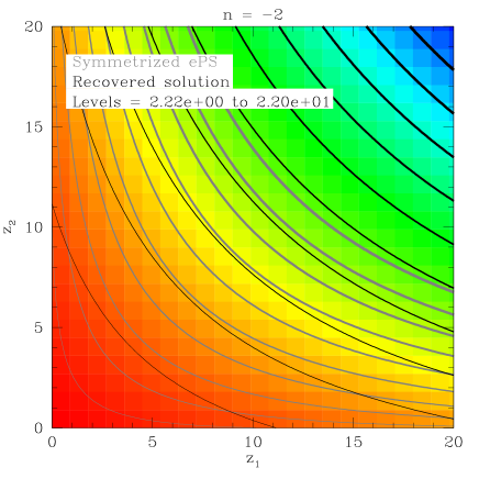
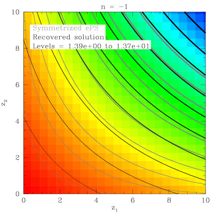
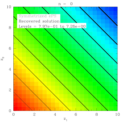
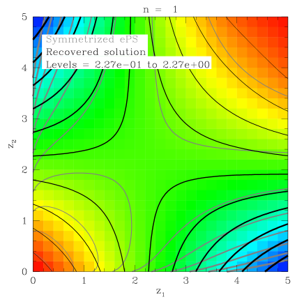
5 Preliminary Results

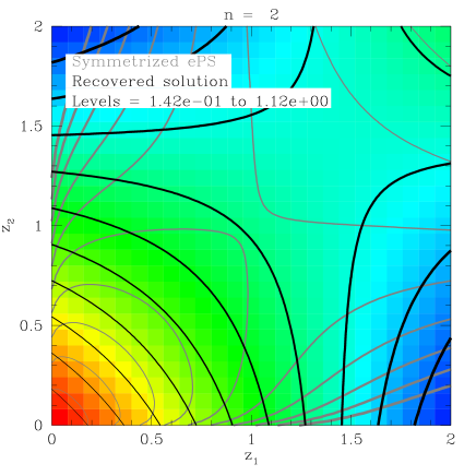
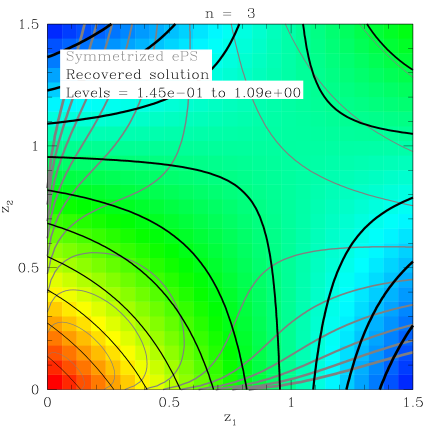
Calculations have been performed for power-law power spectra with $n=-2$, $-1$, $0$, $1$, $2$ and $3$. For the $n=0$ case an exact solution is known, $q(z_{1},z_{2})=(z_{1}+z_{2})/\sqrt{2\pi}$. Figures 2 through 7 show, in their left-hand panels, contour maps of the function $q(z_{1},z_{2})$ recovered by the solution method described above for each value of $n$. The functions are clearly symmetric in their arguments and are all smoothly varying. For contrast, grey lines show a geometrically symmetrized extended Press-Schechter prediction $q_{\rm ePS,sym,G}(z_{1},z_{2})=\left[q_{\rm ePS}(z_{1},z_{2})q_{\rm ePS}(z_{2},z_{1})\right]^{1/2}$, where $q_{\rm ePS}$ is the extended Press-Schechter merger rate corresponding to equation (5). The right-hand panels of these Figures show $y(z)$ predicted by Press-Schechter theory, together with the $y(z)$ determined from the Smoluchowski equation using ${\bf q}$ determined by the techniques described above and using the arithmetically ($q_{\rm ePS,sym,A}(z_{1},z_{2})=\left[q_{\rm ePS}(z_{1},z_{2})+q_{\rm ePS}(z_{2},z_{1})\right]/2$) and geometrically symmetrized extended Press-Schechter kernels. (Note that the results for arithmetically and geometrically symmetrized extended Press-Schechter kernels are indistinguishable in these figures.) In every case we are able to find a symmetric, smoothly varying solution which solves the Smoluchowski equation. The solutions typically differ significantly from the symmetrized extended Press-Schechter prediction, which does not solve the Smoluchowski equation (except for the specific case of $n=0$).

Figure 2: Left-hand panel: The recovered solution for $q(z_{1},z_{2})$ for an $n=-2$ power spectrum is shown as a contour plot (black lines) and by the coloured shading. For comparison, we plot the symmetrized extended-Press-Schechter prediction as grey contours. Contours are drawn between the values indicated in the figure at equal logarithmic intervals (thinnest line corresponding to lowest value). Right-hand panel: The solution, $y(z)$, for an $n=-2$ power spectrum to the Smoluchowski equation. The dashed black line shows the exact Press-Schechter prediction, while the dotted line shows the result found using the Press-Schechter mass function, along with the numerically recovered solution for $q(z_{1},z_{2})$. (Note that these two lines coincide, giving the appearance of a single dot-dashed line.) The solid line shows the result obtained by using the Press-Schechter mass function together with the symmetrized extended Press-Schechter prediction for $q(z_{1},z_{2})$—we plot results for both arithmetically and geometrically symmetrized $q(z_{1},z_{2})$, but the two are indistinguishable in these figures. Note that we plot the absolute value of $y(z)$ and indicate regions where the function becomes negative by thinner lines.

Figure 3: As Fig. 2 but for $n=-1$.

Figure 4: As Fig. 2 but for $n=0$.

Figure 5: As Fig. 2 but for $n=1$.

Figure 6: As Fig. 2 but for $n=2$.

Figure 7: As Fig. 2 but for $n=3$.

The results obtained depend upon several factors:

1. The relative importance given to solving the Smoluchowski equation and meeting the regularization condition when searching for a solution (i.e. the value of $\sigma_{R_{1}}$).

2. The number of elements used in the discretized representation of the Smoluchowski equation and the range of $z$ studied (i.e. $N$ and $\Delta z$). (We have adopted the approach of making $N$ as large as possible given constraints on computing resources, and to make $\Delta z$ as large as possible while retaining sufficient resolution to find an accurate solution to the Smoluchowski equation.)

3. The nature of the regularization condition(s).

The first and second factors can be addressed easily given sufficient computing resources, while the third may require consideration of other constraints that any solution which is to be considered physically reasonable must meet. With the current maximum value of $N=179$ we find that our results change at the 10–20% level if we reduce $N$ to $101$, while changes in $\Delta z$ at fixed $N$ similarly lead to changes in $q(z_{1},z_{2})$ at the 10–20% level. Clearly there is a need to increase $N$ further, or find ways to perform the inversion of the Smoluchowski equation more robustly. We find that our results are quite insensitive to $\sigma_{R_{1}}$ providing it is not made too large or too small (i.e. there is a wide range of $\sigma_{R_{1}}$ over which the results do not change significantly). It seems that the simple condition that the function be smoothly varying is sufficient to obtain physically plausible solutions.

Our results can be described moderately well by the following fitting formula:

$$q(z_{1},z_{2}) = {1\over\sqrt{2\pi}}\left(A_{1}[z_{1}+z_{2}]+A_{2}z_{1}z_{2}\right)$$ (18)

$$\times\exp\left(-A_{4}[z_{1}z_{2}]^{A_{3}}\right),$$

where $A_{1}$, $A_{2}$, $A_{3}$ and $A_{4}$ are free parameters which we determine by fitting to the numerically determined $q(z_{1},z_{2})$. Table 1 lists the values of these parameters. The final column of that table lists the maximum percentage deviation between the fitting formula and the numerical results as shown in Figures 2 through 7. These fitting formulae are valid over the range of $z$ shown in the figures, but cannot be guaranteed to hold for $z$’s outside of these ranges. In particular, for $n>0$ the parameter $a_{2}$ is negative, which will result in $q(z_{1},z_{2})<0$ for certain $z_{1},z_{2}$, which is clearly unphysical. We hope to establish a better fitting formula in future work.

Table 1: Values for the parameters,f $A_{1}$ to $A_{4}$, for the fitting formula given in equation (18) as a function of power-spectrum index, $n$. The final column lists the maximum percentage difference between the fitting formula and the numerical results, when using the values given in the table, over the range of $z_{1}$ and $z_{2}$ shown in Figures 2 through 7.

$n$	$A_{1}$	$A_{2}$	$A_{3}$	$A_{4}$	Max. % deviation
-2	0.502	0.102	-0.450	0.118	15.0
-1	0.809	0.219	-0.504	0.027	8.2
0	1.000	0.000	0.000	0.000	0.0
1	1.239	-0.496	1.580	0.009	14.7
2	1.547	-1.089	-0.555	-0.004	4.9
3	1.997	-2.000	-0.561	-0.005	9.3

It is clear from the right-hand panels of Figs. 2 through 7 that our solutions for $q(z_{1},z_{2})$ produce the correct rate of change of halo abundance. To confirm this we can consider the distribution of halo masses at time $\tau$, $n(z;\tau)$, where $z=M/M_{*}(\tau)$. At time $\tau+\delta\tau$ the distribution of halo masses, using the same definition of $z=M/M_{*}(\tau)$ and not $z=M/M_{*}(\tau+\delta\tau)$, is $n(z;\tau+\delta\tau)=f[\delta\tau]^{2}n(f[\delta\tau]z;\tau)$ where $f(x)=\exp[-6x/(3+n)]$. Using our recovered $q(z_{1},z_{2})$ we can evolve $n(z;\tau)$ to $n(z;\tau+\delta\tau)$ for a small step $\delta\tau$ (such as would be used in a merger tree calculation). We show the results of this test in Fig. 8, which demonstrates our ability to reproduce the evolution of the Press-Schechter mass function using our merger rates. (The figure also demonstrates how poorly the symmetrized extended Press-Schechter estimate of the merging rate does.)

Figure 8: The evolution of the Press-Schechter mass function over a small time step $\delta\tau$ (the value of which is given in each panel). We plot the ratio of the final to initial mass function as a function of mass, $z$. The dashed line shows the expectation from the Press-Schechter theory, while the dotted line shows the result of applying our recovered merger rates to the initial mass function. The solid lines show the results of applying the two symmetrized extended Press-Schechter merger rates to the initial mass function (these two lines are indistinguishable almost everywhere in this figure).

5.1 Some comments on the numerical results

The numerical and ePS merger kernels appear to be monotonically increasing functions of mass for power-law indices $n\leq 0$. However, for power-law indices $n>0$, they appear to peak at masses near the characteristic mass scale $M_{*}$. As expected, the agreement between the numerical and ePS results is exact for $n=0$, and they become increasingly discrepant as $n$ departs from 0. In particular, our numerically-recovered merger kernel disagrees with the ePS merger kernel, and the disagreement increases as $n$ departs from 0. In fact, we attempted to find a numerical merger kernel, demanding that the merger kernel be equal to the ePS merger kernel for equal-mass mergers. However, our algorithm was unable to find a consistent and smooth merger kernel with this constraint. This leads us to believe that the ePS merger rate is invalid, even for equal-mass mergers where the two ePS results agree.

Finally, we point out that ? outline a numerical technique for finding merger kernels, but only under the assumption that the merger kernel is homogeneous; i.e., that the merger kernel can be written in the form $q(z_{1},z_{2})=z_{1}^{m}f(z_{2}/z_{1})$, where $m$ is a power-law exponent. We found that we were able to implement this algorithm and recover the merger kernel for the $n=0$ power spectrum (for which the merger kernel is indeed homogeneous). We then speculated that for more general power-law power spectra, the merger kernel would also be homogeneous. However, we were unable to get the Muralidar-Ramkrishna algorithm to return smooth kernels for these power spectra. Indeed, our numerically recovered merger kernels are not homogeneous for these more general power spectra.

6 Frequently Asked Questions

Below we attempt to answer several questions which frequently arise in connection with this work.

What about three-body encounters? The assumption that halos grow through binary mergers, which is implicit in the Smoluchowski equation, could be questioned. Since the halo abundance diverges at low masses it is possible that a halo will experience an infinite number of mergers per unit time with halos of vanishingly small mass. However, as shown in Appendix A, the creation and destruction rates due to these halos cancel exactly. Therefore, we can truncate the halo mass function at some low mass and obtain a good approximation to the true merging history. Put another way, if the mass distribution is described by discrete objects, as in an N-body simulation, rather than a continuum mass distribution, then there are no three-body mergers. In such a simulation, there could easily be three or more halos that merge within a finite time interval. However, one can always find a sufficiently small time step so that any apparent three-body merger will in fact be a rapid sequence of two-body mergers (somewhat like the triple-alpha reaction in stellar nucleosynthesis, which is in fact a rapid series of two-body reactions).

What can we learn from N-body simulations? In principle, the merger kernel can be determined from N-body simulations. In practice, though, this will be challenging. If we have $N$ mass bins, then there will be $N(N+1)/2$ entries in the merger kernel, and we must have a sufficiently large simulation to provide a statistically significant number of mergers in each of these bins. Such a simulation will also require a very large dynamic range so that a huge number of halos of widely varying masses will be resolved. However, there may be a simpler avenue. If we carry out a constrained realization of a single large halo (see, for example, ?), then the accretion of smaller halos by this single large halo can be used to determine the merger kernel $Q(M_{1},M_{2})$ for a single large $M_{1}$ as a function of $M_{2}$ for $M_{2}\ll M_{1}$. Such a numerical calculation may be helpful in checking the numerical inversion we have carried out here, and perhaps in shedding light on the asymptotic behaviour of $Q(M_{1},M_{2})$ for $M_{2}\ll M_{1}$. We plan to pursue such N-body calculations in future work—initial investigations using simulations with CDM power spectra suggest that our numerical results may better match the N-body merger rates than the predictions of extended Press-Schechter theory.

What about fragmentation? In a realistic N-body simulation, some of the mass in halos might be ejected (e.g., by an analog of the “slingshot” effect). If so, then the coagulation equation should include fragmentation terms. We believe, however, that the fraction of mass ejected will be small, and that the inexorable trend in hierarchical structure formation is to larger masses; this is also mathematically realized in the Press-Schechter and extended Press-Schechter theories. We therefore idealize the situation by neglecting any such fragmentation and attempt to find a solution to the pure coagulation problem first.

What about “smooth” accretion? Some authors have noted that merger trees assembled with the extended-Press-Schechter merger rates do not produce Press-Schechter distributions, as they should, and have thus attempted to account for this discrepancy by the supposition that halos can gain mass by accreting diffuse matter from the smooth intergalactic medium, as well as by mergers with other halos. In our formalism, what others would call “smooth accretion” is described by mergers with very low-mass halos. In other words, every mass element is contained in a halo of some size (as in standard Press-Schechter theory), and smooth accretion is taken into account by mergers with halos of extremely low mass.

Is the numerically determined merger rate unique? Given our choice of regularization condition—namely that the function be as smooth as possible and everywhere positive—we do indeed find a unique solution. However, we could imagine other regularization criteria, perhaps in addition to smoothness and positivity, which would lead to different answers. Not all such criteria may allow a solution to be found. For example, we find that requiring our recovered merger rate to coincide with the extended Press-Schechter merger rate for the case of equal mass mergers prevents us from finding a merger rate which accurately solves the Smoluchowski equation.

Can the merger kernel be determined by looking at the properties (e.g., size) of the physical halos? In most applications of the coagulation equation (e.g., in planetesimal theory), the merger kernel is determined by the physical cross section and relative velocity of the merging objects; i.e., by the “micro”-physics. In our case, however, such a kinetic-theory description will not apply, as the system of halos is “cold” and halos are more likely to merge with those that form nearby, rather than a halo drawn at random from the field. In other words, the merger history is determined by the clustering properties of the halos (as encapsulated by the power spectrum) rather than by any intrinsic property, such as their size.

What about other algorithms for generating merger trees? The fact that the ePS binary merger rates, when used to construct merger trees, do not yield Press-Schechter distributions is well known. There have been algorithms developed that mitigate the shortcomings of ePS by correcting the ePS merger rates with, e.g., three-body mergers or “smooth” accretion (e.g. ?; ?). There is no unique algorithm for constructing a merger tree (? explore many of the possibilities), but some are more successful than others at reproducing the distribution of progenitors of dark-matter halos as predicted by the extended Press-Schechter theory. It should be noted, however, that the merger rates used in these merger trees are not necessarily correct, even if the algorithm does ultimately reproduce the correct mass function. It should be further noted that all of these algorithms rely on the extended Press-Schechter merger rates for major mergers which, as we have shown, are very likely incorrect. As such, these algorithms do not address the problem we consider here. In fact, with our self-consistent merger rates, merger trees can be constructed without resorting to three-body mergers, smooth accretion, or other kluges.

7 Discussion

We have described an approach to find physically reasonable estimates of dark-matter-halo merger rates. We describe techniques for finding numerical solutions to the Smoluchowski coagulation equation which we use to describe the hierarchical formation of dark-matter halos. While the extended Press-Schechter theory contains an intrinsic inconsistency in its predictions for halo merger rates (namely that the merger rate of halos of mass $M_{1}$ with those of mass $M_{2}$ is not the same as that of halos of mass $M_{2}$ with halos of mass $M_{1}$) our approach is guaranteed to always produce self-consistent merger rates.

We have presented symmetric, smooth solutions to the Smoluchowski equation for the case of dark-matter–halo growth through gravitational clustering. These solutions can now be checked against the results of numerical simulations. The same techniques can also be applied to non-power law power spectra (although in general the solution will be somewhat more complex as the merger rate may depend explicitly on time for such power spectra and may contain characteristic mass scales), and also to halo-abundance evolution rates derived from fitting functions designed to reproduce the halo mass functions found in N-body simulations.

A number of questions still remain before we have reliable astrophysical merger rates. First and foremost among these is how to insure that the numerically recovered solution is in fact the solution that correctly describes mergers due to gravitational amplification of an initially Gaussian distribution of perturbations. The fact that our numerical results are highly insensitive to the details of our smoothing constraint leads us to believe that our algorithm is indeed converging to a unique physical result, but we cannot demonstrate this rigorously. Perhaps future analytic work inspired by extended-Press-Schechter–like considerations or N-body simulations may provide insight into constraints, boundary conditions, and/or asymptotic limits that will allow us to confidently zero in on the correct solution. Beyond that, the technique will then need to be applied to obtain a merger kernel for a CDM power spectrum, rather than the scale-invariant power spectra we have considered here. And finally, the merger kernel will ultimately have to be consistent with a Sheth-Tormen or Jenkins et al. mass function, or whatever other mass function is determined to be the “correct” one. With these self-consistent kernels, the well-known problems with ePS formation-redshift distributions (i.e., that they are not positive definite) will be corrected, and merger trees will be easily constructed. We plan to address these issues in future work.

The hierarchical formation of dark-matter halos is a fundamental component of a large fraction of current studies in the fields of cosmology and galaxy formation. A mathematically self-consistent and quantitatively accurate knowledge of halo merger rates is therefore extremely valuable. We believe that the techniques developed in this work may provide a first step for developing such knowledge.

Appendix A Alternative Formulation of the Coagulation Equation

Here we provide an alternative form for the coagulation equation that demonstrates rigorously the cancellation between the divergences in the creation and destruction terms. This form of the equation is for the time evolution for the fraction of the total mass ${\cal F}(<M)$ contained in halos of mass less than $M$. This time evolution can be written,

$${{\rm d}{\cal F}(<M)\over{\rm d}t} ={1\over 2\rho_{0}}\int_{0}^{M}\,{\rm d}M^{\prime}\,M^{\prime}\,$$ (19)

$$\times\int_{0}^{M^{\prime}}{\rm d}M_{1}n(M_{1})n(M^{\prime}-M_{1})Q(M_{1},M^{\prime}-M_{1})$$

$$-{1\over\rho_{0}}\int_{0}^{M}{\rm d}M^{\prime}M^{\prime}n(M^{\prime})$$

$$\times\int_{0}^{\infty}{\rm d}M_{1}n(M_{1})Q(M^{\prime},M_{1}).$$

The first step is to rewrite the first term on the right-hand side as

$${1\over 2}\int_{0}^{M}\,{\rm d}M^{\prime}\int_{0}^{\infty}\,{\rm d}M_{1}\int_{0}^{\infty}{\rm d}M_{2}\,M^{\prime}\delta(M_{1}+M_{2}-M^{\prime})$$

$$\,\,\,\times n(M_{1})n(M_{2})Q(M_{1},M_{2}).$$ (20)

We then carry out the $M^{\prime}$ integral which then changes $M^{\prime}$ in the integrand to $M_{1}+M_{2}$, and changes the upper limits to the $M_{1}$ and $M_{2}$ integrals from $\infty$ to $M$ and $M-M_{1}$, respectively; i.e., this expression is then

$${1\over 2}\int_{0}^{M}\,{\rm d}M_{1}\int_{0}^{M-M_{1}}\,{\rm d}M_{2}\,(M_{1}+M_{2})$$

$$\times n(M_{1})n(M_{2})Q(M_{1},M_{2}).$$ (21)

Since $M_{1}$ and $M_{2}$ enter symmetrically in this expression, it can be replaced by

$$\int_{0}^{M}\,{\rm d}M_{1}\int_{0}^{M-M_{1}}\,{\rm d}M_{2}\,M_{1}n(M_{1})n(M_{2})Q(M_{1},M_{2}).$$ (22)

We then make the replacements $M^{\prime}\rightarrow M_{1}$ and $M_{1}\rightarrow M_{2}$ in the dummy variables in the second term in equation (19) and find that the first and second terms are identical, except for in the limits for the second integral. Combining the two expressions, we find

$$\frac{d{\cal F}(<M)}{dt} = -\int_{0}^{M}\,{\rm d}M_{1}\,M_{1}n(M_{1})$$ (23)

$$\times\int_{M-M_{1}}^{\infty}\,{\rm d}M_{2}\,n(M_{2})Q(M_{1},M_{2}).$$

It is then simple to see that if $n(M)\sim M^{-\gamma}$ with $\gamma<2$ and $Q\sim$ constant as $M\rightarrow 0$, then the divergence in the integrand is integrable.

Appendix B Analytic Solutions to the Smoluchowski Equation

In this Appendix we provide an elementary approach to two known analytic solutions to the Smoluchowski equation. These solutions are not new (see ? for a comprehensive review), but we include them here in the hope that they may provide some insight into more general solutions. We consider the models $q_{ij}=$constant, and $q_{ij}=i+j$. The first leads to an exponential mass function for large times while the second gives the Press-Schechter mass function for an $n=0$ power spectrum.

The Smoluchowski equation is

$$\dot{n}_{1} = -\sum_{i=1}^{\infty}q_{i,1}n_{i}n_{1},$$

$$\dot{n}_{j} = {1\over 2}\sum_{i=1}^{j-1}q_{i,j-i}n_{i}n_{j-i}-\sum_{i=1}^{\infty}q_{ij}n_{i}n_{j},$$ (24)

where $q_{ij}$ corresponds to the discretized coagulation kernel.

We will consider solutions which satisfy the initial conditions

$$n_{1}=1,\quad n_{r}=0\quad r\neq 1.$$ (25)

It will also be useful to define

$$M_{p}(t)=\sum_{j=1}^{\infty}j^{p}n_{j}(t);$$ (26)

i.e., the various moments of the number distribution, as well as the following generating function,

$$F(z,t)=\sum_{j=1}^{\infty}n_{j}(t)\exp(-jz).$$ (27)

We now consider each case individually.

Constant kernel: $q_{ij}=$ const. Inserting the generating function into equation (24) gives

$${\partial F\over\partial t}={F^{2}\over 2}-FM_{0}(t).$$ (28)

The initial conditions imply that $F(z,0)=\exp(-z)$, and setting $z=0$ in equation (28), gives $M_{0}(t)=2/(t+2)$. The generating function can then be solved for:

$$F(z,t)={4\over(t+2)^{2}\exp(z)-t(t+2)}.$$ (29)

Expanding this gives

$$n_{k}(t)={4\over(t+2)^{2}}\Big{(}{t\over(t+2)}\Big{)}^{k-1}.$$ (30)

The asymptotic behaviour of equation (30) is of the form

$$n_{k} \sim t^{-2}g(k/t),\qquad t\rightarrow\infty,$$

$$k = {\mathcal{O}}(t),\qquad g(\eta)=4\exp(-2\eta).$$ (31)

Sum kernel: $q_{ij}=i+j$. Plugging in for the generating function here gives

$${\partial F\over\partial t}={1\over 2}{\partial F\over\partial z}M_{0}(t)-{F\over 2}{\partial F\over\partial z}-{F\over 2}M_{1}(t).$$ (32)

Setting $z=0$ in equation (32) gives $M_{0}(t)=\exp(-t/2)$, and assuming $M_{1}(t)\equiv 1$, we have, via the technique of characteristics (?),

$${\rm e}^{-z}=F\exp\left(1-{\rm e}^{-t/2}+{t\over 2}\right)\exp\left[\left({\rm e}^{-t/2}-1\right)F\right].$$ (33)

The solution is then given using Lagrange’s expansion (?),

$$n_{k}(t)={k^{k-1}\over k!}{\rm e}^{-t/2}\exp[-k(1-{\rm e}^{-t/2})](1-{\rm e}^{-t/2})^{k-1}.$$ (34)

The large-time behaviour can easily be extracted from equation (34) as

$$n_{k}\sim{k^{k-1}\over k!}{\rm e}^{-k}{\rm e}^{-t/2},\qquad t\rightarrow\infty,\qquad k={\mathcal{O}}(1),$$ (35)

and, from Stirling’s formula, as

$$n_{k} \sim {\rm e}^{-2t}g(k/{\rm e}^{t}),\qquad t\rightarrow\infty,$$

$$k = {\mathcal{O}}({\rm e}^{t}),\qquad g(\eta)={{\rm e}^{-\eta/2}\over\sqrt{2\pi\eta^{3}}}.$$ (36)

References

- [Abramowitz & Stegun¡1974¿] Abramowitz M. and Stegun I. A. eds., 1974, “Handbook of Mathematical Functions”, Dover Publications
- [Aldous¡1999¿] Aldous D. J., 1999, Bernoulli, 5, 3
- [Allen & Bastien¡1995¿] Allen E. J., Bastien P., 1995, ApJ, 452, 652
- [Benson et al.¡2002¿] Benson A. J., Frenk C. S., Lacey C. G., Baugh C. M., Cole S., 2002, MNRAS, 333, 177
- [Bond et al.¡1991¿] Bond J. R., Cole S., Efstathiou G., Kaiser N., 1991, ApJ, 379, 440
- [Bond & Myers¡1996¿] Bond J. R., Myers S. T., 1996, ApJS, 103, 63
- [Bower¡1991¿] Bower R. G., 1991, MNRAS, 248, 332.
- [Brent ¡1973¿] Brent R. P., 1973, “Algorithms for Minimization without Derivatives”, Prentice-Hall, Englewood Cliffs, New Jersey
- [Bromm, Coppi & Larson¡1999¿] Bromm V., Coppi P. S., Larson R. B., 1999, ApJ, 527, L5
- [Bullock, Kravtsov & Weinberg¡2000¿] Bullock J. Kravtsov A. Weinberg D. H., 2000, ApJ, 539, 517
- [Cole et al.¡2000¿] Cole S., Lacey C. G., Baugh C. M., Frenk C. S., 2000, MNRAS, 319, 168
- [Gabici & Blasi¡2003¿] Gabici S., Blasi P., 2003, ApJ, 583, 695
- [Gottlober, Klypin & Kravtsov¡1991¿] Gottlober S., Klypin A.,Kravtsov A., 1999, ApSS, 269, 345
- [Haehnelt¡1994¿] Haehnelt M. G., 1994, MNRAS, 269, 1999
- [Jenkins et al.¡2001¿] Jenkins A. et al., 2001, MNRAS, 321, 372
- [Kamionkowski & Liddle¡2000¿] Kamionkowski M., Liddle A. R., 2000, PhRvL, 84, 4525
- [Kolatt et al.¡1999¿] Kolatt T. S. et al., 1999, ApJ, L523, 109
- [Lacey & Cole¡1993¿] Lacey C. G., Cole S., 1993, MNRAS, 262, 627
- [Lacey & Cole¡1994¿] Lacey C. G., Cole S., 1994, MNRAS, 271, 676.
- [Lee¡2000¿] Lee M. H., 2000, Icarus, 143, 74
- [Leyvraz¡2003¿] Leyvraz F., 2003, Phys. Rept., 383, 95
- [Malyshkin & Goodman¡2001¿] Malyshkin L. Goodman J., 2001, Icarus, 150, 314
- [Menou, Haiman & Narayanan¡2001¿] Menou K., Haiman Z., Narayanan V. K., 2001, ApJ, 558, 535
- [Milosavljevic & Merritt¡2001¿] Milosavljevic M., Merritt D., 2001, ApJ, 563, 34
- [Monaco et al.¡2002¿] Monaco P., Theuns T., Taffoni G., Governato F., Quinn T., Stadel J., 2002, ApJ, 564, 8
- [Muralidar & Ramkrishna¡1986¿] Muralidar R., Ramkrishna D., 1986, J. Colloid and Interface Sci., 112, 348
- [Percival et al.¡2003¿] Percival W. J., Scott D., Peacock J. A., Dunlop, J. S., 2003, MNRAS, L338, 31
- [Press & Schechter¡1974¿] Press W., Schechter P., 1974, ApJ, 187, 425
- [Santos, Bromm & Kamionkowski¡2002¿] Santos M. R., Bromm V., Kamionkowski M., 2002, MNRAS, 336, 1082
- [Scannapieco, Schneider & Ferrara¡2003¿] Scannapieco E., Schneider F., Ferrara A., ApJ, 589, 35
- [Sheth¡1995¿] Sheth R., 1995, MNRAS, 274, 213
- [Sheth & Pitman¡1997¿] Sheth R. K., Pitman J., MNRAS, 1997, 289, 66
- [Sheth & Tormen¡1999¿] Sheth R. K., Tormen G., 1999, MNRAS, 308, 119
- [Silk & Takahashi¡1979¿] Silk J., Takahashi T., 1979, ApJ, 229, 242
- [Silk & White¡1978¿] Silk J., White S. D. M., 1978, ApJ, 223, L59
- [Smoluchowski¡1916¿] Smoluchowski M., 1916, Physik. Zeit., 17, 557
- [Somerville¡2002¿] Somerville R. S., 2002, ApJ, 572, 23
- [Somerville & Kolatt¡1999¿] Somerville R. S., Kolatt T. S., 1999, MNRAS, 305, 1
- [Springel et al.¡2001¿] Springel V., White S. D. M., Tormen G., Kauffman G., 2001, MNRAS, 328, 726
- [Stiff, Widrow & Frieman¡2001¿] Stiff D., Widrow L. M., Frieman J., 2001, PhRvD, 64, 3516
- [Verde et al.¡2001¿] Verde L., Kamionkowski M., Mohr J., Benson A. J., 2001, MNRAS, 321, L17
- [Verde, Haiman & Spergel¡2002¿] Verde L., Haiman Z., Spergel D. N., 2002, ApJ, 581, 5
- [Vivitska et al.¡2002¿] Vitvitska M., Klypin A. A., Kravtsov A. V., Wechsler R. H., Primack J. R., Bullock J. S., 2002, ApJ, 581, 799
- [Volonteri, Haardt & Madau¡2002¿] Volonteri M., Haardt F., Madau P., 2002, Ap&SS, 281, 501
- [Wechsler et al.¡2002¿] Wechsler R. H., Bullock J. S., Primack J. R., Kravtsov A. V., Dekel A., 2002, ApJ, 568, 52
- [Wetherill¡1990¿] Wetherill G. W., 1990, Icarus, 88, 336
- [White¡2002¿] White M., 2002, ApJS, 143, 241
- [Wyithe & Loeb¡2003¿] Wyithe S., Loeb A., 2003, ApJ, 595, 614