Lens modelling and $H_{0}$ estimate in quadruply lensed systems

Abstract

We present a numerical method to estimate the lensing parameters and the Hubble constant $H_{0}$ from quadruply imaged gravitational lens systems. The lens galaxy is modeled using both separable deflection potentials and constant mass - to - light ratio profiles, while possible external perturbations have been taken into account introducing an external shear. The model parameters are recovered inverting the lens and the time delay ratio equations and imposing a set of physically motivated selection criteria. We investigate correlations among the model parameters and the Hubble constant. Finally, we apply the codes to the real lensed quasars PG 1115+080 and RX J0911+0551, and combine the results from these two systems to get $H_{0}=56{\pm}23\ {\rm km\ s^{-1}\ Mpc^{-1}}$. In addition, we are able to fit to the single systems a general elliptical potential with a non fixed angular part, and then we model the two lens systems with the same potential and a shared $H_{0}$: in this last case we estimate $H_{0}=49_{-11}^{+6}\ \textrm{Km}\ \textrm{s}^{-1}\ \textrm{Mpc}^{-1}$.

1 Introduction

Gravitational lensing is one of the main tools to obtain information about the structure and evolution of the universe. In particular, time delay measurements are a recent primary distances indicator, furnishing a new method to estimate the Hubble constant $H_{0}$, which determines the present expansion rate of the universe (see, for instance, [Narayan & Bartelmann 1998, Kochanek & Schechter 2003]).

Actually, in 1964, Refsdal proposed to estimate $H_{0}$ [Refsdal 1964a, Refsdal 1964b, Refsdal 1966] from multiply imaged QSOs by the measurements of the delays in the arrive time between light rays coming from the different images, which follow different optical paths. It is not difficult to show that the time delay between two images due to a gravitational lens can be factorized in two pieces: the first one depends on cosmological parameters and is inversely proportional to $H_{0}$, while the second one is determined by the lens model only. Thus, having measured time delays among images of a lensed QSO, once we fix the cosmological parameters, we can obtain a direct estimate of $H_{0}$ provided that the lens model has been recovered from the lensing constraints, or is known in an other independent way. Nowadays, there are more than sixty multiple image systems [CASTLES web page], but only about ten of them have measured time delays. However, this number is increasing day by day, and in the future it will be possible to measure time delays for many other systems.

It is well known hat the most significant uncertainty affecting the estimate of $H_{0}$ with the Refsdal method is only related to the mass model used. In the usual approach the model parameters are recovered by fitting some parametric models to the available constraints through $\chi^{2}$ minimization techniques. Instead, other authors (see [Williams & Saha 2000]) carried out the “pixellated lens” modelling, that describes the mass distribution by a large number of discrete pixels with arbitrary densities, so determining the Hubble constant by means of a set of physical motivated constraints. A compromise between these two approaches consists in the numerical solution of a set of non linear equations: in a previous paper ([Cardone et al. 2002], hereafter CCRP02), for instance, some of us applied a semianalytical technique to fit the separable potential of the form $\psi=r^{\alpha}F(\theta)$ and were able to develop an algorithm to estimate $H_{0}$ without the need to give an explicit expression for the shape function $F(\theta)$.

Here, we further improve the general method in [Cardone et al. 2001] (hereafter CCRP01) and CCRP02, implementing a set of Mathematica codes to shape quadruple lens systems and obtain a better estimate of the Hubble constant. Such a method in fact allows us to manage a still wider class of lens models and to obtain useful information about lens parameters and $H_{0}$, eliminating possible not physical solutions.

Actually, we consider both separable models, specifying the angular part $F(\theta)$, and models with constant mass-to-light ratio. As usually in literature, we develop the potential of an external object contributing to the lensing phenomenon to second order, and hence its effect on the total deflection potential translates into an external shear term [Schneider, Ehlers & Falco 1992]. We constrain the lens models using the image positions with respect to the lens centre and the time delay ratios, which allow us to highly constrain the used models, even if the equations to be solved become more complex. Once the results from all the possible models are collected together, such a procedure offers the advantage of giving an estimate of the Hubble constant which is in a sense marginalized with respect to the lens models.

Moreover, our numerical method allows to pursue a new kind of approach to the lens modelling, that considers at the same time several lens systems. Actually, following [Saha & Williams 2004], we try to model two lensed systems with the elliptical potential $\psi=r^{\alpha}F(\theta)$ and an external shear, based on a strong hypothesis we make ab initio: we suppose that the lens systems has a shared $H_{0}$. In this way we are able to create a two-system model that can give a more complete estimate of $H_{0}$.

The outline of the paper is as follows. In Sect. 2 we write the lens equations and the time delay function in polar coordinates. A careful presentation of the models we use is given in Sect. 3, while Sect. 4 is devoted to the presentation of the numerical method used to ‘fit’ single lens models to systems. We also discuss the constraints used to select physically motivated solutions and the statistical approach to obtain the final estimate of the parameters. Then in Sect. 5 we present a new approach to shape two lens systems with a shared $H_{0}$. In order to verify whether our codes are able or not to recover the correct values of parameters, we build simulated systems to which we apply the codes as described in Sect. 6, where, in addition, we analyze the biases and the uncertainties in the use of a model respect to another one. In Sect. 7, we use the simulated systems to investigate the existence of degeneracies among the model parameters, recovering some interesting scaling laws. Sect. 8 is dedicated to the application of our procedure to two real quadruple systems, PG 1115+080 and RX J0911+0551: we obtain an estimate of the lensing parameters and the Hubble constant, also taking into account the contribution of changing the cosmological parameters to the uncertainty on $H_{0}$. Finally, we present a discussion of our results and future improvements in Sect. 9.

2 Lens equation and time delay

Let us choose a rectangular system $(x,y)$ centered on the lens galaxy and with axes pointing towards West and North, respectively. Let $(r,\theta)$ be the polar coordinates, being $\theta$ the position angle measured from North to East, connected to the rectangular ones through the following coordinate transformation:

$$x=-r\sin\theta,\hskip 14.22636pty=r\cos\theta\ .$$ (1)

Time delay function, i.e. time delay of a generic path from source to observer, is given by [Blandford & Narayan 1986, Zhao & Pronk 2001]:

$$\Delta t=h^{-1}\tau_{100}$$ (2)

$$\bigg{[}\frac{1}{2}r^{2}-rr_{s}\cos(\theta-\theta_{s})+\frac{1}{2}r_{s}^{2}-\psi(r,\theta)\bigg{]},$$

where $(r,\theta)$ determines the impact position of the generic path on the lens plane (with $r$ measured in arcsec), $(r_{s},\theta_{s})$ is the unknown source position, and $\psi(r,\theta)$ is the adimensional lensing potential. Then, $h$ is the Hubble constant $H_{0}$ in units of $100\ {\rm km\ s^{-1}\ Mpc^{-1}}$, while $\tau_{100}$ is a typical time delay linked to cosmological parameters, and defined as:

$$\tau_{100}\equiv\frac{D_{d}D_{s}}{D_{ds}}\frac{1+z_{d}}{c},$$ (3)

where $D_{d}$, $D_{s}$ and $D_{ds}$ are observer - lens, observer - source, and lens - source angular diameter distances, calculated with $H_{0}=100\ {\rm km\ s^{-1}\ Mpc^{-1}}$, and $z_{d}$ is the lens redshift. This factor contains all the cosmological information, since the distance depend on the other cosmological parameters: i.e. the density matter parameter $\Omega_{m}$, the “dark energy” contribution $\Omega_{X}$ (see [Peebles & Ratra 2002, Caldwell, Dave & Steinhardt 1998, Demianski et al. 2003]) and the smoothness parameters $\tilde{\alpha}$ introduced in [Dyer & Roeder 1972, Dyer & Roeder 1973, Dyer & Roeder 1974] to take into account the inhomogeneities of the universe. If $i$ and $j$ are two images, the time delay between them is $\Delta t_{ij}=\Delta t_{i}-\Delta t_{j}$.

According to Fermat principle, the images lie at the critical points of $\Delta t$, so one can obtain lens equations minimizing it. We get:

$$r-r_{s}\cos(\theta-\theta_{s})=\frac{\partial\psi}{\partial r},$$ (4)

$$r_{s}\sin(\theta-\theta_{s})=\frac{1}{r}\frac{\partial\psi}{\partial\theta}.$$ (5)

We shall use a lensing potential formed by the sum of two terms:

$$\psi(r,\theta)=\psi_{lens}(r,\theta)+\psi_{ext}(r,\theta),$$ (6)

where $\psi_{lens}(r,\theta)$ is the contribution of the lens galaxy, and $\psi_{ext}(r,\theta)$ is the external perturbation. The first term is connected with the mass distribution of the galaxy through the Poisson equation:

$$\nabla^{2}\psi_{lens}(r,\theta)=2\kappa(r,\theta),$$ (7)

being $\kappa(r,\theta)$ the convergence, i.e., the adimensional surface mass density, defined as:

$$\kappa(r,\theta)\equiv\frac{\Sigma(r,\theta)}{\Sigma_{crit}},$$ (8)

where $\Sigma_{crit}=\frac{c^{2}D_{s}}{4\pi GD_{d}D_{ds}}$. The second term describes the effects on the lensing system of the environment, i.e., of the cluster of galaxies which the lens galaxy belongs to, or an external group of galaxies. We describe this contribution developing the lensing potential of the external perturbation to the second order:

$$\psi_{ext}(r,\theta)=\psi_{shear}(r,\theta)=-\frac{1}{2}\gamma r^{2}\cos 2(\theta-\theta_{\gamma}),$$ (9)

where $\gamma$ is the external shear and $\theta_{\gamma}$ is the shear angle, oriented from North to East and pointing towards the external perturbation.

3 Lens models

The majority of the lens galaxies are early-type galaxies, since lensing selects galaxies by mass and the fact that early type galaxies are more massive than spirals overwhelms the fact that spirals are slightly more numerous. Early type galaxies show a wide variety of optical shapes including oblate, prolate and triaxial spheroids. Moreover, also their mass distribution is not yet fully understood: stellar dynamics and X ray observations all suggest that the early type galaxies are dominated by dark matter halos; on the other hand, some dynamical studies recently performed using planetary nebulae as tracers in the halos of early-type galaxies show evidence of a universal declining velocity dispersion profile, and dynamical models indicate the presence of little dark matter within $5R_{e}$ – implying halos either not as massive or not as centrally concentrated as CDM predicts [Romanowsky et al. 2003]. So not only a fundamental hypothesis of the CDM paradigm have been remained up to now largely unverified – that there should be similarly extended, massive dark halos around ellipticals –, but predictions about the detailed halo properties have not been testable. Gravitational lensing is actually an unique tool to studying elliptical halos, and face the question about the nature and the distribution of dark matter in early type galaxies, with implications on the estimation of the Hubble constant. In order to consider both a luminous-dominated and dark-dominated component in the main lens galaxy, we consider two different classes of models : separable potentials and constant mass - to - light ($M/L$) mass profiles.

Table 1: Separable deflection potentials.

Model	$\psi(r,\theta)$
Model 1	$\frac{b^{2-\alpha}}{\alpha}r^{\alpha}$
Model 2	$b\sqrt{\sin(\theta-\theta_{q})^{2}+q^{-2}\cos(\theta-\theta_{q})^{2}}\hskip 2.84544ptr$
Model 3	$\frac{b^{2-\alpha}}{\alpha}\sqrt{\sin(\theta-\theta_{q})^{2}+q^{-2}\cos(\theta-\theta_{q})^{2}}\hskip 2.84544ptr^{\alpha}$

3.1 Separable potentials

For the first class, we assign the lensing potential in a simple separable form:

$$\psi(r,\theta)=r^{\alpha}\ F(\theta,q,\theta_{q})\ ,$$ (10)

where we have explicitly indicated the dependence of the angular part $F(\theta,q,\theta_{q})$ on the axial ratio $q$ ($0<q<1$) and the position angle $\theta_{q}$ that specifies the orientation of the lensing galaxy. The potentials (10) are a generalization of the pseudoisothermal elliptical potentials (PIEP) studied by [Kovner 1987]. This kind of model is in many aspects similar to the pseudoisothermal elliptic mass distribution (PIEMD) models, such as the singular isothermal ellipsoid (SIE) [Blandford & Kochanek 1987]. However, while PIEMD models can represent mass models with any elongation, PIEP models represent physically plausible lenses only for some values of the axial ratio $q$, such as $q>q_{0}$, being $q_{0}$ a suitable value of the axial ratio of the isopotential contours [Kovner 1987, Kassiola & Kovner 1995]. For $q<q_{0}$, the elliptical isodensity profile may in fact be boxy or disky. In particular, when dealing with these elliptical models, we adopt the following expression for the angular part:

$$F\propto\left[\sin^{2}(\theta-\theta_{q})+q^{-2}\cos^{2}(\theta-\theta_{q})\right]^{1/2},$$ (11)

where $\theta_{q}$ is oriented from West to North. The angular part $F$ also depends on a strength parameter b: for a singular isothermal sphere ($\alpha=1$ and $F=$const) this parameter depends on the cosmological parameters and the redshifts by means of a distance ratio, and on the central velocity dispersion. In our case we can assume a similar dependence only for Model 3 (see Table 1).

In Table 1 we give the expression of $\psi$ for the three different models we consider. Model 1 is spherically symmetric, and hence the shape function is $F=\frac{b^{2-\alpha}}{\alpha}$. On the other hand, both Model 2 and 3 are ellipticals, but for Model 2 we fix $\alpha=1$ as for isothermal mass distributions, while $\alpha$ is unfixed for Model 3.

It is worth to note that, since the lensing potential $\psi$ and the adimensional surface density $\kappa$ are related by a double integration, the ellipticity of the isopotential contours is different by that of isodensity ones. Therefore, we have to obtain a relation between the axial ratio $q$ of the potential and the isodensity axial ratio, named $q_{\kappa}$. For Model 2, the convergence is:

$$\kappa(r,\theta)=\frac{bq}{2r}(\cos^{2}(\theta-\theta q)+q^{2}\sin^{2}(\theta-\theta q))^{-\frac{3}{2}}\ .$$ (12)

It is easy to see that $\kappa$ is always positive, i.e., Model 1 is always correctly defined, and the analytical relation $q_{\kappa}=q^{3}$ holds. Things get more complicated for Model 3. The convergence now turns out to be:

$$\kappa(r,\theta)=\frac{b^{2-\alpha}r^{-2+\alpha}}{4q\alpha}[2(-1+q^{2}+\alpha^{2})\cos^{4}(\theta-\theta q)$$

$$+q^{2}(2(1+q^{2}(-1+\alpha^{2}))\sin^{4}(\theta-\theta q)+\alpha^{2}\sin^{4}2(\theta-\theta q))]$$

$$\ \ \ {\times}[(\cos^{2}(\theta-\theta q)+q^{2}\sin^{2}(\theta-\theta q))]^{-\frac{3}{2}}\ .$$ (13)

It is possible to see that, if one of the two factors $q^{2}(\alpha^{2}-1)+1$ and $q^{2}+\alpha^{2}-1$ is negative, then is $\kappa<0$. In particular, if $\alpha>1$, we always have $\kappa>0$, since the two quantities above are positive; instead, when $\alpha<1$, the convergence $\kappa$ is negative if $q<\sqrt{1-\alpha^{2}}$. For instance, if $\alpha=0.5$ and $q<0.866$, the convergence is negative. The axial ratio $q_{\kappa}$ satisfies the relation

$$q_{\kappa}=\bigg{(}\frac{q(-1+q^{2}+\alpha^{2})}{-q^{2}+1+q^{2}\alpha^{2}}\bigg{)}^{\frac{1}{2-\alpha}},$$ (14)

that corresponds to more rapid trends for lower values of $\alpha$.

3.2 Constant $M/L$ models

The second class we consider contains models that describe luminosity profiles of elliptical galaxies. We use the de Vaucouleurs [de Vaucouleurs 1948] and Hubble (REF) models (respectively Model 4 and 5), whose convergence $\kappa$ is given in Table 2. We assume that the mass density is spherically symmetric, so that we can avoid any difficulties in solving the lens equations for these models. Given the surface density $\kappa$, the deflection angle is easily obtained as [Schneider, Ehlers & Falco 1992, Keeton 2001]:

$$\hat{\alpha}(r)=\frac{2}{r}\int_{0}^{r}r^{\prime}dr^{\prime}\kappa(r^{\prime}),$$ (15)

and then the deflection potential is evaluated solving the equation $\hat{\alpha}=\nabla\psi$.

Table 2: Mass distribution for constant $M/L$ models. For the de Vaucouleurs model see Keeton & Kochanek 1997.

Model	$\kappa$
Model 4	$\frac{b}{R_{e}N^{\prime}}e^{[-7.67(\frac{r}{R_{e}})^{\frac{1}{4}}]}$
Model 5	$\frac{1}{2}\frac{b^{2}}{s^{2}+r^{2}}$

4 Single system modelling

Developing the general method used in CCRP01 and CCRP02 to model quadruply lensed systems, we numerically solve systems of nonlinear equations, imposing on the sample of solutions some criteria to select only the physical ones, that have to be collected together by means of an appropriate statistical analysis.

4.1 Method

Here, we consider separable models with an assigned angular part and more complex mass models for which it is necessary to assign the surface density $\kappa$. In order to take into account all of the information that come from a lensing event, we make use of time delay ratios, that allow to constrain the lensing parameters quite efficiently. We do not use flux ratios since these may be contaminated by microlensing [Chang & Refsdal 1979, Koopmans & de Bruyn 2000], and other effects, such as those due to substructures in the lens galaxy [Mao & Schneider 1998]. Instead, time delays are well measured for some quasars with great accuracy and are less affected by spurious (and uncontrollable) effects. The unknown parameters to be determined are the source position $(r_{s},\theta_{s})$, the shear quantities ($\gamma,\theta_{\gamma})$, the main lens model parameters (different for each model), and the Hubble constant $H_{0}$. Actually, the higher complexity of the models and the introduction of the time delays as constraints lead to more complicated equations than those considered in CCRP01 and CCRP02, and it is not possible to manipulate them to reduce the set of lensing equations (2), (4) and (5) to a simpler form so as to speed up the calculations. Let us write equations (4) and (5) using the four images $i$, $j$, $k$ and $l$, and the two equations coming from the time delay ratios among them, that are independent on h:

$$\frac{\Delta t_{ik}}{\Delta t_{ij}}=\frac{\Delta t_{ik}^{obs}}{\Delta t_{ij}^{obs}},\qquad\frac{\Delta t_{il}}{\Delta t_{ij}}=\frac{\Delta t_{il}^{obs}}{\Delta t_{ij}^{obs}},$$ (16)

where $\Delta t_{ij}^{obs}$, $\Delta t_{ik}^{obs}$ and $\Delta t_{il}^{obs}$ are the measured time delays. The introduction of these two other equations permits to rise the equations number, allowing to give a different constraint by the images positions that does not depend on the first derivative of the potential, but only on the potential.

In summary, we consider the observables without the errors, using their mean values: while for the image positions this assumption seems immediately justified, for the time delays the uncertainties can be considerably large. In a next section, we will show more accurately which this assumption is reasonable.

We have a number of 10 equations (8 from lens equations and the 2 due to the time delay ratios), that we combine in a useful manner to reduce their number to the unknowns number. For example, in the case of $Model\;1$ the unknowns are 6, i.e., $r_{s}$, $\theta_{s}$, $\gamma$, $\theta_{\gamma}$, $b$, and $\alpha$, with in addition the Hubble constant. We have to subtract the 8 lens equations to reduce their number to 4, and we then add the two time delay ratios to complete the system of 6 equations in 6 unknowns. We use the same procedure for each model to obtain a system of $n$ equations and $n$ unknowns. We can numerically solve this system of $n$ equations to obtain $n$ unknown parameters (for our models $n$ is less than 10). Each result of the solution of the system will be a set of $n$ values. When we go to solve the system, we do not obtain a single solution, but a set of solutions, since the system is highly non linear; these solutions have to be selected by means of some selection criteria in order to obtain values of parameters which give rise to physically plausible models.

The search for the roots of the system begins with a choice of a range of parameter values: one must be sure that there are no roots outside the chosen range, and also a very large interval does not necessarily include all roots, increasing CPU time. We choose a physically acceptable interval for parameters, giving $\mathcal{N}$ random starting points to the algorithm, where $\mathcal{N}$ is a number fixed by the user. From these starting points the CPU tries to converge to the solutions, using the Newton’s method. In particular, to assign the same probability to the starting values of a parameter in the relative range, we generate these values uniformly distributed, also to avoid introducing any bias in the search.

We have developed a simple code, named LePRe, Lensing Parameters Reconstruction, written for Mathematica. Generally, solving the equation system yields $\mathcal{M}<\mathcal{N}$ solutions, because for some values of the starting points Newton’s method fails to converge to a solution.

4.2 Selection criteria

These $\mathcal{M}$ solutions are not all physically acceptable and to sort among these we have to impose a set of selection criteria, that constrains parameter values to physically plausible ranges. Schematically, we can describe these selection criteria as following.

1. $0<r_{s}<max\{r_{i},r_{j},r_{k},r_{l}\}$: a lens will not produce images arbitrarily far away from the center of the lens; for large values of $r_{s}$, there will be one image only at $(r,\theta)=(r_{s},\theta_{s})$, and possibly others near the center of the lens; in particular, we impose this cut because if the source is outside the ring delineated by the most distant of the images it is not possible to generate a 4-images configuration.

2. $0<\gamma<\gamma_{crit}$: the shear magnitude is positive by definition. For the separable models, we choose as upper limit $\gamma\approx\gamma_{crit}$, where $\gamma_{crit}$ is defined such that for values of $\gamma\geq\gamma_{crit}$ the estimated $H_{0}$ becomes null, and depends on the particular lens system to be considered [Wucknitz 2002]. For PG 1115+080 is $\gamma_{crit}=0.22$, instead for RX J0911+0551 is $\gamma_{crit}=0.56$. For axially symmetric lenses we cannot fix an upper limit (since the hypothesis made in [Wucknitz 2002] does not work), but in the analysis it is possible to obtain estimated value of $\gamma$ higher than the one obtained for an elliptical separable model.

3. The shear is approximately well directed: we mean that the position angle $\theta_{\gamma}$ must be directed towards the external mass disturbance; e.g., if the shear were due to an external group of galaxies, then $\theta_{\gamma}$ should be aligned with the cluster mass centre, since there are no reasons why it should point elsewhere. For the axially symmetric models this cut is not necessary because an exact value of $\theta_{\gamma}$ is selected automatically from the system solution to account for image configuration. Instead, for an elliptical model, we have to take into account the degeneracy existing between external asymmetry (the shear $\gamma$ and relative orientation $\theta_{\gamma}$) and internal asymmetry provided by axial ratio $q$ and angle $\theta_{q}$. Quantitatively, one could accept only values comprised in the range $(\theta_{G\,min},\theta_{G\,max})$, where $\theta_{G\,min}$ and $\theta_{G\,max}$ are respectively two extreme galaxies that bound the external group of galaxies.

4. The elliptical profile of the galaxy has to be physically plausible: we assume $q_{0}<q<1$, where $q_{0}$ is a particular value of $q$ such that, for fixed value of $\alpha$, the isodensity profile is elliptical or nearly elliptical, and not strongly boxy; so, we avoid those kinds of solutions to select the physically plausible one.

5. The range for other galaxy model parameters is chosen to have plausible values of $\kappa$. For Model 1 and Model 3 we must have $0<\alpha<2$; as a matter of fact, the surface mass density scales as $r^{\alpha-2}$, so that $\alpha<2$ is needed in order to have $\kappa$ monotonically decreasing with $r$. On the other hand, we consider $\alpha>0$ in order for the projected mass inside $r$ (that scales as $r^{\alpha}$) to be reasonable. Since $\psi>0$, we have to assume the condition $b>0$ for the strength parameter.

6. Plausible index ind($\kappa$). The index is the logarithmic derivative of $\kappa$, i.e., $ind(\kappa)\equiv\frac{d\log\kappa}{d\log r}$. A lower bound can be fixed considering that $\kappa$ has to be higher than the luminous profile; an upper bound for PG 1115+080 is fixed following [Williams & Saha 2000], i.e., $ind(\kappa)<-0.5$. For power law model this selection criterium reduces to $\alpha<1.5$.

7. The set of parameters so found solves lens equations and time delay ratios equations. We insert the solutions in solved equations, to check if the solution found is the correct one or a result from wrong convergence of the numerical algorithm. We impose that the values of parameters so found verify the equations within an accuracy fixed by the user.

8. $h_{min}<h<h_{max}$. From the three time delays we obtain three values of $h$ ($h_{ij}$, $h_{ik}$ and $h_{il}$), and eliminate all the solutions such that the predicted values of these three $h$’s differ more than an $\epsilon$ ($=0.1$) from each other. Then, we estimate $h\equiv(h_{ij}+h_{ik}+h_{il})/3$, selecting only those solutions which give rise to values of $h$ in the range $(h_{min},h_{max})$, being these two parameters fixed by the user. An upper bound is given by age of globular clusters and by the limits from nucleochronology, which indicate an age of the Universe of $t_{0}>7.8\ Gyr$; instead, a lower bound on $h$ can be given by $t_{0}\approx 20\ Gyr$, since we do not observe stellar systems with ages greatly exceeding this value. In particular, to be conservative, we choose $(h_{min},h_{max})=(0,2)$.

Obviously, one can also change the order of the constraints, and remove or add some of these. At the end of the application of such selection criteria, and after having run the code more times, we get a set of $\mathcal{L}$ solutions. It is clear that there is a family of different combinations of the parameters, that is consistent with the observables and the selection criteria.

4.3 Statistical interpretation

It is possible to interpret the final sample of the solutions for each parameter using the concept of Bayesian probability. In this particular framework, the lensing parameters and $H_{0}$ represent the “variables” of the “system”, that are linked by a series of “relationships”, that need not be single-valued, i.e., the lens mapping and time delay equations. We can associate to the “variables” a single value function, that is usually named “information”, or more familiarly “probability density function”, which indicates how “likely” the particular combination of the parameters is. Our final sample of solutions, collected into the histograms, determines all the amount of “information” that we obtain about the “system” itself. This sample is a subset of the parameter space, that contains all we have to know about the “system”. To extract a final result, we have to select a better estimate of each parameter, making a reasonable choice. We could use a figure of merit as made by [Saha & Williams 1997], but here we use the mean value of all the collected values as final estimate for each parameter, instead for the uncertainty on this estimate we think to be conservative in the choice of the 68% confidence level, i.e., the range in which the 68% of the solutions is included. In the first place, this choice works well in the simulations. Then, we argue that our choice allows to take into account the weight of each single result in the sample. When the distribution of the values is symmetric, other choices as the maximum or the median are equivalent, but in some cases the histograms have a degree of asymmetry, different for each lensing model and quasar system, due to the particular configuration of the images, the degeneracies and the available data.

As we said before, by means of a simulated system, we will see that this estimate of the uncertainty in the parameter determinations in fact allows us to recover the values of these ones.

5 A ‘two-system’ model

In a recent paper, Saha & Williams extract an estimate of $H_{0}$ by means of the joined use of more lensed systems [Saha & Williams 2004]. Here, we show how it is possible to build a ‘two-system’ model fitting two lens systems with general lensing potentials and a shared $H_{0}$. In order to obtain a simpler solution to this problem we use an elliptical potential with a not fixed angular part $F_{unk}(\theta)$ and external shear

$$\psi=F_{unk}(\theta)r^{\alpha}+\psi_{shear},$$ (17)

already used in CCRP02. As shown in that paper, if we do not assign the angular part of the potential, it is possible to write the time delay between two images i and j in a simple form and, in particular, for $h_{ij}$ the relation

$$h_{ij}=\frac{1}{\Delta t_{ij}^{obs}}\frac{\tau_{100}}{2\alpha}[(\alpha-2)(r_{i}^{2}-r_{j}^{2})$$ (18)

$$+2(1-\alpha)r_{s}(r_{i}\cos(\theta_{i}-\theta_{s})-r_{j}\cos(\theta_{j}-\theta_{s}))$$

$$+(\alpha-2)\gamma(r_{i}^{2}\cos 2(\theta_{i}-\theta_{\gamma})-r_{j}^{2}\cos 2(\theta_{j}-\theta_{\gamma}))],$$

holds, where the lens parameters related to the angular trend of the lens galaxy do not appear, but only the source position, the shear, the parameter $\alpha$, and the normalized Hubble constant $h_{ij}$. The choice of this potential allows us not only to explore a wide range of models but also to obtain equations with a more little number of unknowns and then more simply solvable.

We impose that the $h^{\prime}s$ due to different pairs of images and the two different systems (i.e., $h_{ij}^{(1)}$, $h_{ik}^{(1)}$, $h_{il}^{(1)}$, $h_{ij}^{(2)}$, $h_{ik}^{(2)}$ and $h_{il}^{(2)}$) are equal. We could solve a system of equations of the form $h_{ij}^{(1)}=h_{ik}^{(1)},\,h_{ij}^{(1)}=h_{ij}^{(2)},\,h_{ij}^{(2)}=h_{ik}^{(2)},\,.....$, in order to obtain the 10 parameters $r_{s}^{(1)},\theta_{s}^{(1)},\gamma^{(1)},\theta_{\gamma}^{(1)},\alpha^{(1)},r_{s}^{(2)},\theta_{s}^{(2)},\gamma^{(2)},\theta_{\gamma}^{(2)},\alpha^{(2)}$. We verified, anyway, that it is better to introduce a figure of merit of the form

$$\Gamma=(h_{ij}^{(1)}-h_{ik}^{(1)})^{2}+(h_{ij}^{(2)}-h_{ik}^{(2)})^{2}+(h_{ij}^{(1)}-h_{ij}^{(2)})^{2}+...,$$ (19)

and we minimize it. We calculate the derivatives with respect to the 10 lens parameters and solve this system of 10 equations. Following the previous section, we impose some selection criteria to select the physical solutions. In this case, in order to reject many unphysical solutions we have to impose a criterion not used previously: i.e., we require that the source has a more constrained position. This criterion is not arbitrary, since the source can be located only in a little region to be able to generate a particular configuration of the images (see [Saha & Williams 2003]). After having obtained a sample of solutions we have to calculate the six $h^{\prime}s$ by different pairs of images and the two systems, and perform the mean of these values; finally, we impose the constraint on $h^{\prime}s$ and obtain the final sample of solutions, that gives out the estimates of the parameters.

We want to stress the fact that the algorithm discussed in this Sec. and hence the developed method, has as main issue the estimate of $h$. It does not allow to obtain precise estimate of the position of the source and of the orientation of the external perturbation, since we impose a strong constraint on them, primary in order to obtain the correct estimate of $h$. As we will see later, it also gives us a good determination of the other parameters (i.e., $\gamma$, $\alpha$, and $h$).

We will compare the results with those obtained by using a similar function of merit to model the single lens systems with the same elliptical potentials. In this case the function $\Gamma$ is simply modified introducing only the terms with the index $(1)$.

6 Application to simulated systems

In this section we verify the correct working of the codes, simulating real systems with image positions and time delays exactly known (i.e., without observational uncertainties). Later on, analyzing the system PG 1115+080, we will show that this last assumption is reasonable, also for the real systems.

6.1 Simulations

For each simulation we fix the system parameters and obtain the image positions and the three time delays by solving the lens equations (4) and (5), and evaluating the time delay function. We use these quantities as input for the codes in order to verify if they are able to recover the correct values of the originally fixed parameters.

Table 3: Simulated and estimated parameters, the angles are written in radiants.

	Model 1	Model 2	Model 3	Model 4	Model 5
$r_{s}^{est}\hskip 2.27626pt$	$0.09_{-0.02}^{+0.02}$	$0.4_{-0.02}^{+0.01}$	$0.20_{-0.07}^{+0.03}$	$0.21_{-0.02}^{+0.02}$	$0.15_{-0.01}^{+0.02}$
$r_{s}\hskip 2.27626pt$	$0.09$	$0.4$	$0.20$	$0.20$	$0.15$
$\theta_{s}^{est}\hskip 2.27626pt$	$6.98_{-0.01}^{+0.01}$	$2.48_{-0.06}^{+0.02}$	$2.701_{-0.004}^{+0.004}$	$5.00_{-0.01}^{+0.01}$	$4.5_{-0.002}^{+0.002}$
$\theta_{s}\hskip 2.27626pt$	$6.98$	$2.5$	$2.7$	$5.00$	$4.5$
$\gamma^{est}$	$0.2_{-0.04}^{+0.04}$	$0.19_{-0.09}^{+0.02}$	$0.15_{-0.08}^{+0.01}$	$0.16_{-0.02}^{+0.02}$	$0.15_{-0.01}^{+0.02}$
$\gamma$	$0.2$	$0.2$	$0.15$	$0.15$	$0.15$
$\theta_{\gamma}^{est}\hskip 2.27626pt$	$3.77_{-0.01}^{+0.01}$	$3.01_{-0.02}^{+0.09}$	$6.32_{-0.12}^{+0.03}$	$1.67_{-0.01}^{+0.01}$	$3.8_{-0.001}^{+0.004}$
$\theta_{\gamma}\hskip 2.27626pt$	$3.77$	$3$	$6.34$	$1.66$	$3.8$
$q^{est}$	$-$	$0.89_{-0.04}^{+0.01}$	$0.9_{-0.01}^{+0.01}$	$-$	$-$
$q$	$-$	$0.9$	$0.9$	$-$	$-$
$\theta_{q}^{est}\hskip 2.27626pt$	$-$	$2_{-0.4}^{+0.1}$	$2.29_{-0.11}^{+0.05}$	$-$	$-$
$\theta_{q}\hskip 2.27626pt$	$-$	$2$	$2.3$	$-$	$-$
$b^{est}$	$0.81_{-0.11}^{+0.08}$	$1.8_{-0.1}^{+0.1}$	$1.6_{-0.4}^{+0.7}$	$1.76_{-0.57}^{+0.84}$	$0.95_{-0.21}^{+0.06}$
$b$	$0.8$	$1.8$	$1.5$	$1.5$	$1$
$\alpha^{est}$	$0.99_{-0.16}^{+0.17}$	$-$	$1_{-0.1}^{+0.4}$	$-$	$-$
$\alpha$	$1$	$-$	$1$	$-$	$-$
$s^{est},\hskip 0.28436ptR_{e}^{est}\hskip 0.28436pt$	$-$	$-$	$-$	$0.51_{-0.27}^{+0.45}$	$0.17_{-0.14}^{+0.05}$
$s,\hskip 0.28436ptR_{e}\hskip 0.28436pt$	$-$	$-$	$-$	$0.6$	$0.2$
$h^{est}$	$0.69_{-0.18}^{+0.05}$	$0.69_{-0.04}^{+0.08}$	$0.67_{-0.22}^{+0.20}$	$0.66_{-0.10}^{+0.10}$	$0.73_{-0.03}^{+0.08}$
$h$	$0.7$	$0.7$	$0.7$	$0.7$	$0.7$

In these simulation we adopt a flat homogeneous universe with cosmological constant, fixing:

$$(\Omega_{m},\Omega_{\Lambda},\Omega_{k},h)=(0.3,0.7,0.0,0.7)\ ,$$ (20)

and:

$$(z_{d},z_{s})=(0.31,1.722),$$ (21)

giving $\tau_{100}=33.37\hskip 2.84544pt\textrm{days}\hskip 2.84544pt\textrm{arcsec}^{-2}$.

In addition to the expected solution, that is recovered with high accuracy, the application of the codes generates other solutions, different by the first one, due to the existence of the degeneracies among the lensing parameters, that we will describe in the next Section. The statistics on this solutions generates our estimate of each parameter. Therefore, the uncertainties of the parameters in the simulations and the real cases are not generated by a sort of propagation of the errors of the observables, but are instead the result of the degeneracies.

The application of the method to simulated systems allows to verify how well it works in recovering the lens parameters and the normalized Hubble constant h. We resume the results in Table 3, where we report the simulated values of the parameters and the estimated ones.

Finally, we show the distributions of the values of $h$ for the 5 models, adding the total distribution, obtained averaging the single distributions, in Figure 1. In particular, we can obtain a “marginalized” estimate of $h$ averaging the distributions, taking into account all the recovered values in the distributions, and giving them finite weights: if $N_{i}(h)$ indicates the distribution of the i-th model, the combined $N(h)$ is given through a mean; this final distribution takes into account the different weights for the different models.

We obtain the global result $h_{est}=0.69{\pm}0.11$. We may in fact consider this procedure a way to obtain a final estimate of the Hubble constant unaffected by spurious uncertainties of the single codes, having taken into account different kinds of models and the whole parameters space. In this way, we can see that the final estimate of $h$ is affected by a lower uncertainty.

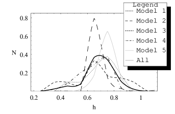
Figure 1: Distributions of the recovered values of the Hubble constant. N indicates a number of values normalized to the total number of results obtained for each model. This definition for $N$ will be used for all the following continuous distributions. The distributions are obtained interpolating the recovered histograms.

We have to verify whether the algorithm for the model with a common $h$ is able or not to recover the lens parameters and, in particular, the Hubble constant. The results are reported in Table 4: it is possible that some parameters are not perfectly recovered, but the main ones are obtained with good accuracy.

Table 4: Simulated and estimated parameters for the model with a not fixed angular part (Two-systems model).

	simulated	estimated
$r_{s}^{(1)}$	$0.25$	$0.28_{-0.14}^{+0.13}$
$\theta_{s}^{(1)}$	$1.6$	$1.66_{-0.49}^{+0.33}$
$\gamma^{(1)}$	$0.13$	$0.13_{-0.06}^{+0.04}$
$\theta_{\gamma}^{(1)}$	$3.00$	$2.98_{-0.14}^{+0.31}$
$\alpha^{(1)}$	$1.1$	$1.13_{-0.13}^{+0.14}$
$r_{s}^{(2)}$	$0.15$	$0.24_{-0.16}^{+0.18}$
$\theta_{s}^{(2)}$	$2.8$	$2.90_{-0.36}^{+0.44}$
$\gamma^{(2)}$	$0.15$	$0.13_{-0.08}^{+0.03}$
$\theta_{\gamma}^{(2)}$	$3.00$	$2.96_{-0.30}^{+0.06}$
$\alpha^{(2)}$	$1$	$1.06_{-0.09}^{+0.19}$
$h$	$0.7$	$0.68_{-0.14}^{+0.13}$

In addition, we verify the correct working of the code when we fit the same potential to a single simulated system. The results are reported in Table 5. We note that the estimate of $h$ for the two-system model has a lower uncertainty than that of the single modelling

Table 5: Simulated and estimated parameters for the model with $F(\theta)$ unknown, fitted to a single system.

	simulated	estimated
$r_{s}^{(1)}$	$0.25$	$0.25_{-0.18}^{+0.19}$
$\theta_{s}^{(1)}$	$1.6$	$1.70_{-0.47}^{+0.28}$
$\gamma^{(1)}$	$0.13$	$0.12_{-0.10}^{+0.06}$
$\theta_{\gamma}^{(1)}$	$3.00$	$2.96_{-0.33}^{+0.53}$
$\alpha^{(1)}$	$1.1$	$1.20_{-0.22}^{+0.27}$
$h$	$0.7$	$0.66_{-0.18}^{+0.19}$

6.2 Model reconstruction from other lens models

It is well known that the main uncertainty in applying the gravitational lensing in order to estimate the Hubble constant and to investigate the astrophysical properties of the galaxies comes from the lack of knowledge of the “true” galaxy model (see, for instance, [Schneider, Ehlers & Falco 1992]). Here, we want briefly to analyze the biases and the errors due to the use of an “incorrect” parametric model to fit the observable data. A way to face this important question consists in to build simulated systems for a lens model and then to fit the image positions and time delays generated by it, using an other functional form, studying the change in the lens parameters and above all in $h$. We can furnish a qualitative estimate of the effect of the model dependence on $H_{0}$. At the same time the procedure allows to quantify this “systematic” errors.

By means of a simulated system built using the Hubble model, we fit to the image positions and the time delays so obtained the Model 1 and Model 2. The analysis of the most significant parameters shows interesting trends which are partially already well known. In particular, in our simulated system $h=0.7$, and the fitting of the other models gives us the means values $h=0.35$ for the Model 1 and $h=0.46$ for the Model 2, respectively with a percentage change of $50\%$ and $34\%$. This percentage obviously changes if we simulate other lens systems. This shows that if the “correct” model for a lens is one with constant mass-to-light ratio and it tries to shape it with a separable model we obtain a lower estimate of $h$ than that obtained with the first one; this verifies some previous results in literature (see [Kochanek 2002] for an analysis made on real systems). Similar trends are obtained if we create a simulated system using a de Vaucouleurs model. It is also possible to analyze the uncertainties introduced by the lack of the internal ellipticity of the lens galaxy. If we try to fit with the Model 1 the observables generated with the Model 2 we obtain a lower mean $h$ but if we consider the errors this estimate is in agreement with the simulated value, instead the estimated value for $\alpha$ raises.

7 Parameter degeneracies

By means of simulated systems we can also obtain statistical correlations among parameters in order to investigate the degeneracies among them and to study the effect of varying each parameter on the final Hubble constant estimate. Below, we discuss the results we found for each model.

• Model 1. We see that $r_{s},\gamma,b$, and $h$ correlate each other, and anticorrelate with $\alpha$. In particular, we verify the scaling laws [Wucknitz 2002]:

  $$r_{s}\propto 2-\alpha,\hskip 7.11317pt\gamma\propto 2-\alpha\hskip 7.11317pt,\hskip 7.11317pth\propto 2-\alpha.$$ (22)

  Wucknitz & Refsdal 2001 give a simple interpretation for these scaling laws in terms of mass-sheet degeneracy. In Figure 2 we report as an example the correlation $h-\alpha$, fitting the line $h=a(2-\alpha)$, where $a$ is a proportionality constant.

  

  Figure 2: Scaling law $h\propto 2-\alpha$ for Model 1.

• Model 2. For this isothermal model we observe that $r_{s},b$, and $h$ correlate among each other, and anticorrelate with $\gamma$ and $q$; almost all of these are linear correlations with a high correlation degree. We note (see also later considerations about correlations for Model 3) that the absence of the parameter $\alpha$ changes the correlations among the shear $\gamma$ and the other parameters, i.e., since $\alpha$ is fixed, $\gamma$ now correlates negatively with $r_{s},b$, and $h$, and not positively.

• Model 3. $r_{s},\gamma,q,b$, and $h$ correlate among each other and anticorrelate with $\alpha$. Here, the positive correlation among $\gamma$ and the other parameters comes back: this allows us to confirm that, in Model 2, it is the condition $\alpha=1$ that changes the correlations of the external shear and not the presence of an intrinsic ellipticity. We also note the obvious positive correlation between $q$ and $\gamma$ (as for Model 2). Higher values of the internal ellipticity (i.e., lower values of $q$) require lower values of $\gamma$.

• Model 4. For the de Vaucouleurs model we find similar linear correlations: $r_{s},\gamma,b$, and $h$ correlate among each other and anticorrelate with $R_{e}$, which now assumes the role of $\alpha$. For example, for higher values of $R_{e}$, this model predicts lower values of Hubble constant.

• Model 5. For the Hubble model we find the same correlations of the preceding model, simply replacing $R_{e}$ with the core radius $s$

For real systems it is more difficult to obtain these correlations. Therefore, we do not discuss the results for them, and we prefer to resume the obtained dependencies in the following:

• The parameters $r_{s}$, $b$, and $h$ always correlate positively among each other; i.e., more massive lenses require higher values of the radial position of the source and of the Hubble constant. The observations show that more luminous galaxies give larger angular separations of the images, in agreement with our correlations: a larger $b$ generates a larger $r_{s}$ and, hence, a larger separation of the images.

• The parameters that determine the radial profile of the lens galaxy ($\alpha$, $R_{e}$, or $s$) correlates negatively with the other ones.

• Except for the Model 2, all the models reveal a positive correlation of the shear with $r_{s}$, $b$, and $h$.

8 Application to PG 1115+080 and RX J0911+0551

Having checked that the numerical codes indeed work correctly recovering the values of the lensing parameters and Hubble constant, we apply them to real quadruply imaged systems. We need a four images system with a good astrometry of the lensing galaxy and image positions, and time delays measured with high accuracy. Then, we also need that there is a single galaxy acting as lens: for instance, with our models we cannot study a gravitational lens like B 1608+656, since there are two lensing galaxies; in this case, a more complex (two) lens model should be used. There are only three systems that satisfy all these requirements: PG 1115+080, RX J0911+0551, and B 1422+231. Here, we choose to apply the codes only to PG 1115+080 and RX J0911+0551, since B 1422+231 has time delays measured with a high uncertainty (see, for instance [Patnaik & Narasimha 2001]). We will also combine the results from the two systems to get a better estimate of the Hubble constant. We adopt a flat cosmology with $(\Omega_{m},\Omega_{\Lambda})=(0.3,0.7)$, discussing for each system the influence of changing the cosmological parameters on the final estimate of $H_{0}$.

8.1 Application to PG 1115+080

PG 1115+080 was discovered by [Weymann et al. 1980], originally as a triple lensed quasar. Later, it has been possible to split an image (the image A) in two components, $A_{1}$ and $A_{2}$. Therefore, this system consists of four images ($A_{1}$, $A_{2}$, $B$, and $C$) of a radio quiet QSO at $z_{s}=1.722$, with an elliptical galaxy as lens belonging to a group of galaxies at $z_{d}=0.31$. This group, situated at South-West, contains $\sim$ 11 galaxies, with a luminous centroid at $(r_{g},\theta_{g})=(20^{\prime\prime}{\pm}0.2^{\prime\prime},-117^{o}{\pm}3^{o})$. Iwamuro et al. fitted the luminous profile of the lensing galaxy with a de Vaucouleurs model with $R_{e}=0^{\prime\prime}.58{\pm}0^{\prime\prime}.05$, and measured an ellipticity $\sim 0.1$ and a position angle of $\sim 65^{0}$ from north [Iwamuro et al. 2000].

Here, we use image coordinates measured by [Impey et al. 1998], and the time delay obtained by [Barkana 1997]. In particular, in [Barkana 1997] it measured a time delay between the components $B$ and $C$ of $\Delta t_{BC}=25.0{\pm}1.7$ days, consistent with the previous value $23.7{\pm}3.4$ days from [Schechter et al. 1997]. By contrast, the time delay ratio $r_{ABC}=\Delta t_{AC}/\Delta t_{BA}=1.13^{+0.18}_{-0.17}$ found by Barkana is in conflict with the value $0.7{\pm}0.3$ from [Schechter et al. 1997].

We can fit this system with the models previously discussed and observe some peculiar trends in the obtained parameter values, that we discuss in the following:

• The source positions are consistent with each other except for Model 2, that has a little disagreement in its mean value.

• As expected, axially symmetric models predict a higher mean value of the shear, to account for the lack of an internal asymmetry, being in agreement with the previous estimates of $\sim 0.1$. It is also interesting to note that $\theta_{\gamma}$ is perfectly oriented towards the luminous centroid of the external group.

• The isopotential profile has a small ellipticity, which increases when we go to consider the relative isodensity profiles. In particular, Model 2 predicts an E0 - E1 galaxy, while Model 3 is also consistent with more elliptical profiles. Instead, $\theta_{q}$ marginally agrees with the luminous profile orientation, but is nonetheless in agreement with results obtained with other techniques [Impey et al. 1998].

• We obtain $\alpha$ values consistent (also if marginally) with the nearly isothermal model, with major preference for Model 3 (see [Kochanek 2002]).

• Model 4 predicts a value of $R_{e}$ in agreement with the measured one of $0^{\prime\prime}.58{\pm}0^{\prime\prime}.05$ by [Iwamuro et al. 2000], while for Model 5 the core radius $s$ is very small, being consistent with a null core within the uncertainties.

• At least, the most important result concerns the estimated Hubble constants. Constant $M/L$ models predict higher values than separable models, as yet found previously in literature [Courbin et al. 1997, Kochanek 2002]. Then, for the isothermal Model 2, we verify a result of [Impey et al. 1998] that gives a low value using a SIE, an isothermal model similar to our model, but with a different angular part.

We report the results of the application of our procedure in Fig. 3. In Fig. 4 we group together the different distributions. The mean distribution gives the value $H_{0}=58{\pm}27\ {\rm km\ s^{-1}\ Mpc^{-1}}$. The mean distribution for the constant mass-to-light ratio models gives us $H_{0}=73{\pm}22\ {\rm km\ s^{-1}\ Mpc^{-1}}$ in according with the recent results in [Kochanek 2002]. If we change the values of cosmological parameters, our final estimate can change of $\sim 3\%$, but the spread becomes $\sim 12\%$ if we also consider inhomogeneous models.

Table 6: Estimated parameters for PG 1115+080. $\theta_{q}$ is oriented from West to North.

	Model 1	Model 2	Model 3	Model 4	Model 5
$r_{s}\hskip 2.27626pt(^{\prime\prime})$	$0.14_{-0.05}^{+0.05}$	$0.10_{-0.02}^{+0.02}$	$0.16_{-0.09}^{+0.08}$	$0.17_{-0.02}^{+0.02}$	$0.19_{-0.05}^{+0.08}$
$\theta_{s}\hskip 2.27626pt(^{o})$	$24_{-3}^{+3}$	$18_{-6}^{+5}$	$21_{-5}^{+5}$	$24_{-4}^{+2}$	$24_{-2}^{+2}$
$\gamma$	$0.15_{-0.05}^{+0.05}$	$0.09_{-0.03}^{+0.02}$	$0.13_{-0.10}^{+0.07}$	$0.16_{-0.03}^{+0.02}$	$0.17_{-0.04}^{+0.04}$
$\theta_{\gamma}\hskip 2.27626pt(^{o})$	$-114_{-3}^{+2}$	$-115_{-8}^{+15}$	$-119_{-7}^{+11}$	$-114_{-4}^{+2}$	$-115_{-3}^{+3}$
$q$	$-$	$0.97_{-0.03}^{+0.02}$	$0.95_{-0.06}^{+0.04}$	$-$	$-$
$q_{k}$	$-$	$0.91_{-0.08}^{+0.06}$	$0.70_{-0.19}^{+0.25}$	$-$	$-$
$\theta_{q}\hskip 2.27626pt(^{o})$	$-$	$155_{-21}^{+41}$	$180_{-22}^{+60}$	$-$	$-$
$b$	$1.06_{-0.07}^{+0.05}$	$0.98_{-0.10}^{+0.16}$	$1.05_{-0.14}^{+0.19}$	$1.51_{-0.41}^{+0.8}$	$0.50_{-0.13}^{+0.20}$
$\alpha$	$0.62_{-0.44}^{+0.50}$	$-$	$0.70_{-0.50}^{+0.70}$	$-$	$-$
$s,\hskip 0.28436ptR_{e}\hskip 0.28436pt(^{\prime\prime})$	$-$	$-$	$-$	$0.72_{-0.37}^{+0.48}$	$0.11_{-0.10}^{+0.30}$
$h$	$0.54_{-0.21}^{+0.19}$	$0.33_{-0.08}^{+0.09}$	$0.59_{-0.30}^{+0.34}$	$0.62_{-0.08}^{+0.11}$	$0.84_{-0.20}^{+0.25}$

Figure 3: Histograms of the recovered values of the Hubble constant for PG 1115+080. The area under the histograms is normalized to unity.

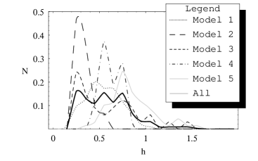
Figure 4: Distributions of all the recovered values of the Hubble constant for PG 1115+080.

Finally, in order to verify the honesty of our assumption of considering the observables without errors, we proceed as following: we consider as input values for the codes the mean values of the observables, and then, we change the time delays of an amount about the 15%. For example, for the Model 1 we obtain the results in figure 5. The two best values of h are: $h_{down}=0.50^{+0.16}_{-0.21}$ and $h_{up}=0.64^{+0.23}_{-0.25}$, in agreement with each other and with the value obtained using the central value. Therefore, the uncertainty in the time delays is extensively absorbed by the uncertainty due to the parameter degeneracies.

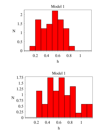
Figure 5: Histograms of the recovered values of the Hubble constant for PG 1115+080 with Model 1 changing the time delays.

8.2 Application to RX J0911+0551

RX J0911+0551 was discovered by [Bade et al. 1997] as a quadruple imaged QSO, in the ROSAT All-Sky Survey (RASS). The source QSO is situated at $z_{s}=2.8$, while the lensing galaxy is at $z_{d}=0.77$. The image configuration is peculiar: the three images $A_{1}$, $A_{2}$ and $A_{3}$ are close to each other and to the lensing galaxy ($A_{1}-A_{2}=0.478^{\prime\prime}$, $A_{2}-A_{3}=0.608^{\prime\prime}$), while image $B$ is more distant than the lens, requiring a large external shear. The only intrinsic ellipticity does not allow to account for this configuration, and we need an external asymmetry. There is, in fact, a nearby group at about $38^{\prime\prime}$ South-West, and at redshift $z_{group}=0.7{\pm}0.1$ that can be the origin of this external perturbation. [Hjort et al. 2002] measured the time delay obtaining the results $\Delta t_{BA_{1}}=-143{\pm}6\hskip 2.84544pt\textrm{days}$, $\Delta t_{BA_{2}}=-149{\pm}6\hskip 2.84544pt\textrm{days}$ and $\Delta t_{BA_{3}}=-154{\pm}16\hskip 2.84544pt\textrm{days}$. It is also possible to observe a second galaxy near the main one, that can affect the modelling.

In the following we present the main results of the application of our codes:

• The models predict nearly the same values for the source positions, except Model 3, that provides a lower value.

• The axially symmetric model yields a high value of the shear; for Model 2 we obtain $\gamma=0.22$, while Model 3 requires a lower value. The shear angle points towards the external group, allowing for the particular configuration observed.

• The elliptical model requires a density distribution with high ellipticity consistent with an E1 - E5 galaxy, with a position angle oriented towards the external group.

• Model 1 gives a lower value of $\alpha$ in agreement with the value from [Schechter 2000], while for the other elliptical model this value is high to account for the low values of $\gamma$ and $q$.

• The effective radius $R_{e}$ is low ($\sim 0.2$), and the core radius of the Hubble model is consistent with zero.

• The recovered value of $H_{0}$ are higher than those obtained using PG 1115+080, with dramatically high uncertainties. The distributions of these values are too much flat giving us a little quantity of statistical information; maybe, using more complex models and other constraints we could improve these results.

Our method allows to obtain the better estimate for the system parameters, but this circumstance does not also allow us to claim that a particular model fits the image positions and the other observables with higher accuracy. We note that the axially symmetric models are able to recover the correct position of the images $A_{1}$, $A_{2}$ and $A_{3}$, but do not allow to get the position of the fourth image due to lacking of internal ellipticity.

Table 7: Estimated parameters for RX J0911+0551.

	Model 1	Model 2	Model 3	Model 4	Model 5
$r_{s}\hskip 2.27626pt(^{\prime\prime})$	$0.60_{-0.14}^{+0.21}$	$0.50_{-0.16}^{+0.16}$	$0.29_{-0.17}^{+0.20}$	$0.52_{-0.12}^{+0.24}$	$0.49_{-0.15}^{+0.19}$
$\theta_{s}\hskip 2.27626pt(^{o})$	$87_{-6}^{+6}$	$88_{-6}^{+4}$	$87_{-7}^{+8}$	$85_{-7}^{+10}$	$84_{-7}^{+5}$
$\gamma$	$0.42_{-0.09}^{+0.07}$	$0.22_{-0.15}^{+0.07}$	$0.17_{-0.13}^{+0.28}$	$0.42_{-0.08}^{+0.10}$	$0.38_{-0.11}^{+0.12}$
$\theta_{\gamma}\hskip 2.27626pt(^{o})$	$171_{-3}^{+3}$	$173_{-7}^{+11}$	$181_{-22}^{+36}$	$170_{-5}^{+4}$	$168_{-6}^{+6}$
$q$	$-$	$0.88_{-0.08}^{+0.08}$	$0.80_{-0.15}^{+0.15}$	$-$	$-$
$q_{k}$	$-$	$0.68_{-0.17}^{+0.20}$	$0.68_{-0.20}^{+0.24}$	$-$	$-$
$\theta_{q}\hskip 2.27626pt(^{o})$	$-$	$88_{-42}^{+44}$	$81_{-29}^{+48}$	$-$	$-$
$b$	$0.96_{-0.08}^{+0.09}$	$1.11_{-0.26}^{+0.23}$	$0.94_{-0.56}^{+0.54}$	$6.34_{-4.36}^{+5.33}$	$0.38_{-0.12}^{+0.23}$
$\alpha$	$0.20_{-0.17}^{+0.38}$	$-$	$1.42_{-0.90}^{+0.33}$	$-$	$-$
$s,\hskip 0.28436ptR_{e}\hskip 0.28436pt(^{\prime\prime})$	$-$	$-$	$-$	$0.18_{-0.14}^{+0.18}$	$0.06_{-0.06}^{+0.36}$
$h$	$0.99_{-0.28}^{+0.40}$	$1.00_{-0.40}^{+0.44}$	$0.57_{-0.33}^{+0.52}$	$0.75_{-0.35}^{+0.41}$	$0.83_{-0.46}^{+0.59}$

We may also try to apply an iterative procedure to verify the correct working of the codes for this lens system. We fix the values of almost all the parameters leaving two of them free. Then, we choose one of those two, solving the lens equation relative to the image $B$ and obtaining an estimate for the other parameter. After finding this value, we can iterate the process solving the equation for the other parameter. After that, we again calculate the image position without being able to recover the correct ones. Therefore, we argue that is not possible to fit the image positions with an axial symmetric model with external shear.

Our results agree with [Burud et al. 1998]; they show that the particular image configuration requires a minimum ellipticity for the galaxy of $\epsilon_{min}=0.075$ and a minimum shear of $\gamma_{min}=0.15$, applying the method of [Witt & Mao 1997]. In particular, we predict very high values of $\gamma$, except for Model 2 and Model 3, that needs a lower mean value, but in agreement with that lower bound.

The histograms of the $H_{0}$ values are shown in Figs. 6. We collect all the distributions in Fig. 7. We give two final estimates of Hubble constant, the first one only including the elliptical models, and the second one including all models. Using the elliptical models we obtain $H_{0}=81{\pm}41\hskip 2.84544pt\textrm{km}\hskip 1.42271pt\textrm{s}^{-1}\textrm{Mpc}^{-1}$, instead taking into account all the models we have $H_{0}=77{\pm}43\hskip 2.84544pt\textrm{km}\hskip 1.42271pt\textrm{s}^{-1}\textrm{Mpc}^{-1}$. Using a power-law model with external shear (the “ Yardstick” model) [Schechter 2000] gets a low value of $\alpha$, in agreement with the value obtained for Model 1, and $H_{0}=42\hskip 2.84544pt\textrm{km}\hskip 1.42271pt\textrm{s}^{-1}\textrm{Mpc}^{-1}$, with an uncertainty $\sim 10-20\%$. This value does not agree with the result obtained here because in [Schechter 2000] is used a time delay of $200\hskip 2.84544pt\textrm{days}$ among the mean image $A$ and the image $B$, different by the one we use. Instead, including in the model the main lens galaxy, the cluster of galaxy, and individual galaxies in the cluster [Hjort et al. 2002] get an estimate of $H_{0}=71{\pm}4\hskip 2.84544pt(\textrm{random},2\sigma){\pm}8\hskip 2.84544pt(\textrm{systematic})\hskip 2.84544pt\textrm{km}\hskip 1.42271pt\textrm{s}^{-1}\textrm{Mpc}^{-1}$, that agrees with the value we obtain.

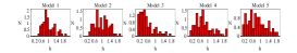
Figure 6: Histograms of the recovered values of the Hubble constant for RX J0911+0551.

Fixing other values for cosmological parameters, the maximum spread is $\sim 10\%$, but considering a Dyer & Roeder universe we have a value $\sim 30-40\%$, since the redshifts $z_{s}$ and $z_{d}$ of RX J0911+0551 are higher than those of PG 1115+080. Actually, RX J0911+0551 is not the ideal system to obtain an accurate estimate of $H_{0}$, since there is a high uncertainty introduced by the arbitrary choice of different cosmological parameters.

Finally, we remark that a simple elliptical potential with external shear, also being able to account for image configuration, is an approximate attempt to model a complex system as RX J0911+0551. Our modelling, in fact, allows to obtain useful information about the system, but we expect to obtain better results using, for example, a SIS or SIE to describe the contribution of the external group, and not an approximation as the external shear. Moreover, it is necessary to take into account the contribution of the second galaxy and the other objects in the group.

8.3 Marginalized estimate of $H_{0}$

For each systems we obtained an estimate of $H_{0}$ performing a mean of the final distributions obtained fitting each model, and then deriving the mean value and the uncertainty from it. Now, let us combine these results, multiplying the two final distributions. The final estimate turns out to be :

$$H_{0}=56{\pm}23\hskip 2.84544pt\textrm{km}\hskip 1.42271pt\textrm{s}^{-1}\textrm{Mpc}^{-1}.$$ (23)

The uncertainties in each estimate and in the final one are high (also if reduced in this last one with respect to the single systems), since it has to take into account all the degeneracies; however, adding other physical constraints and strengthening some of those already used, it is possible to reduce the errors ulteriorly. Also for the lens parameters there is this kind of problem, above all in the orientation of the lens galaxy and the strength parameters of some models. We think that this kind of “marginalized” estimate of $H_{0}$ over a large sample of models can help us to overcome the problem of the lack of a correct independent knowledge of the lens model.

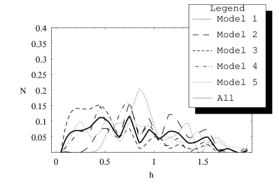
Figure 7: Distributions of all recovered values of the Hubble constant for RX J0911+0551.

8.4 Application of the two-system model

In addition to the usual analysis done for each system, we apply to PG 1115+080 and RX J0911+0551 the new method to simultaneously fit the general elliptical model $\psi=F(\theta)r^{\alpha}$ with external shear. In Table 8 we collect the results, adding the values obtained for the single systems fitted with the same potential. The uncertainties in the estimated value for RX J0911+0551 are very high as well as for the other models fitted in the paper, showing the presence of difficulties in the fitting performed with these simple models. The angular trends for the two-system model and the single systems are similar and there is an agreement for the estimated $\alpha^{\prime}s$. The global estimate of the Hubble constant is $H_{0}=49_{-11}^{+6}\ Km\ s^{-1}\ Mpc^{-1}$. Its determination is mainly determined by the uncertainties in the estimate of $H_{0}$ for PG 1115+080, since the distribution of the recovered for RX J0911+0551 is flat, giving us a little quantity of information (see, for instance, Fig. 8).

Table 8: Estimated parameters for the fitting of the elliptical potential with not fixed angular part (two-systems model), and comparison with the results obtained fitting the same potential to the single systems.

	Two-systems	PG 1115+080	RX J0911+0551
$r_{s}^{(1)}\hskip 2.27626pt(^{\prime\prime})$	$0.25_{-0.14}^{+0.36}$	$0.22_{-0.17}^{+0.12}$	$-$
$\theta_{s}^{(1)}\hskip 2.27626pt(^{o})$	$23_{-38}^{+26}$	$31_{-41}^{+26}$	$-$
$\gamma^{(1)}$	$0.10_{-0.05}^{+0.01}$	$0.09_{-0.06}^{+0.03}$	$-$
$\theta_{\gamma}^{(1)}\hskip 2.27626pt(^{o})$	$-108_{-31}^{+9}$	$-113_{-30}^{+8}$	$-$
$\alpha^{(1)}$	$1.13_{-0.15}^{+0.19}$	$1.17_{-0.21}^{+0.22}$	$-$
$r_{s}^{(2)}\hskip 2.27626pt(^{\prime\prime})$	$0.24_{-0.18}^{+0.12}$	$-$	$0.39_{-0.30}^{+0.28}$
$\theta_{s}^{(2)}\hskip 2.27626pt(^{o})$	$108_{-18}^{+15}$	$-$	$100_{-42}^{+22}$
$\gamma^{(2)}$	$0.11_{-0.10}^{+0.14}$	$-$	$0.25_{-0.16}^{+0.13}$
$\theta_{\gamma}^{(2)}\hskip 2.27626pt(^{o})$	$171_{-28}^{+24}$	$-$	$184_{-26}^{+18}$
$\alpha^{(2)}$	$1.59_{-0.12}^{+0.13}$	$-$	$1.42_{-0.40}^{+0.35}$
$h$	$0.49_{-0.11}^{+0.06}$	$0.45_{-0.11}^{+0.06}$	$0.62_{-0.38}^{+0.28}$

These final values, but in particular the first one, are in good agreement with the previous ones in the literature. The results obtained by some of us in previous papers are also consistent with the present ones: in CCRP01 it was obtained $H_{0}=56_{-11}^{+12}\hskip 2.84544pt\textrm{km}\hskip 1.42271pt\textrm{s}^{-1}\textrm{Mpc}^{-1}$, using an elliptical potential without external shear and only PG 1115+080, while in CCRP02 it has been found a value of $H_{0}=58_{-15}^{+17}\hskip 2.84544pt\textrm{km}\hskip 1.42271pt\textrm{s}^{-1}\textrm{Mpc}^{-1}$, fitting a general elliptical potential to PG 1115+080 and B 1422+231. Using the pixellated lens method, Williams & Saha the results from PG 1115+080 and B 1608+656 are combined to finally get $H_{0}=61{\pm}11\hskip 2.84544pt\textrm{km}\hskip 1.42271pt\textrm{s}^{-1}\textrm{Mpc}^{-1}$, in good agreement with our result. Using a $\chi^{2}$ minimization applied to B1608+656, [Koopmans & Fassnacht 1999] get $H_{0}=65_{-6}^{+7}\hskip 2.84544pt\textrm{km}\hskip 1.42271pt\textrm{s}^{-1}\textrm{Mpc}^{-1}$, only marginally in agreement with our result. In [Treu & Koopmans 2002] it is obtained $H_{0}=59_{-7}^{+12}{\pm}3\hskip 2.84544pt\textrm{km}\hskip 1.42271pt\textrm{s}^{-1}\textrm{Mpc}^{-1}$, modelling PG 1115+080 with two different components so as to describe the luminous part and the dark halo, and using information by stellar dynamics.

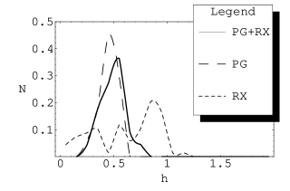
Figure 8: Distributions of all recovered values of the Hubble constant for the model withb $F(\theta)$ unknown, applied to the two systems.

9 Conclusions

In this paper we have presented a numerical method able to estimate lensing parameters and Hubble constant for a wide class of models. The model parameters as well as the Hubble constant have been estimated using as constraints the image positions and the time delay ratios. We used two classes of models: separable elliptical models and constant mass - to - light ratio profiles, adding an external shear to take into account the presence of an external group of galaxy. For these models we solved the system composed by the combinations of lens equations and two time delay ratios, selecting the solutions by means of suitable physical constraints. For each model and each parameter, we obtain an ensemble of values: we used the mean as better estimate and a confidence level of $68\%$ as error. In order to reduce the uncertainty due to the lens models on the estimation of the Hubble constant, we marginalized over all the models collecting the complete data set and obtained a final estimate of $H_{0}$ and its error, which does not result dramatically underestimated, in this way, because of an a priori choice of the model. To test the code we created simulated systems, being able to recover the correct values of parameters.

After the encouraging testing of the codes, we have then applied them to two real systems for which a measure of time delays has been possible: PG 1115+080 and RX J0911+055. For PG 1115+080 it was possible to get an estimate of $H_{0}=58{\pm}27\hskip 2.84544pt\textrm{km}\hskip 2.84544pt\textrm{s}^{-1}\textrm{Mpc}^{-1}$, consistent with other results in the literature, obtained using different techniques. For example, [Courbin et al. 1997, Keeton & Kochanek 1997] show that the isothermal and pseudoisothermal models predict low values of $H_{0}$, while the constant mass - to - light ratio ones generate higher values. We can verify these results using Hubble and de Vaucouleurs models, finding that a simple elliptical isothermal model as Model 2 predicts a very low value of $H_{0}$, in agreement with the value $\sim 40\hskip 2.84544pt\textrm{km}\hskip 2.84544pt\textrm{s}^{-1}\textrm{Mpc}^{-1}$ obtained in [Impey et al. 1998]. For RX J0911+0551, only the elliptical profile allows to fit the image configuration. These trends are also confirmed by the simulations.

As previously said, we “marginalize” over the models since we do not know the “correct” form of the lens model, and hence we have thought to overcome this difficulty in this way. The combination of the two final distribution can help to reduce the uncertainties and to obtain more information from more lens systems, thus should avoid the problems in the fitting of the single systems. The combined estimate is $H_{0}=56{\pm}23\hskip 2.84544pt\textrm{km}\hskip 2.84544pt\textrm{s}^{-1}\textrm{Mpc}^{-1}$

The uncertainty in the final estimate can be further reduced adding other models and including in the statistics other lensed systems, consistently with the uncertainty obtained using other methods (see, for instance, [Williams & Saha 2000]). If we consider the contribution of the smoothness parameter $\tilde{\alpha}$, the change in $H_{0}$ can be very high and comparable with uncertainty in our estimates of $H_{0}$. For example, the variability for RX J0911+0551 is $\sim 30-40\%$ (using these particular cosmological models), with a comparable uncertainty in modelling.

The general method developed in this paper can be used to do more, allowing to obtain an estimate of $H_{0}$ that is assumed for hypothesis as the ‘same’ for all the lensed systems (see [Saha & Williams 2004]). We can in fact fit simultaneously the two systems, using a general elliptical potential with a not fixed angular part and a shared $H_{0}$. The final estimate is $H_{0}=49_{-11}^{+6}\ \textrm{Km}\ \textrm{s}^{-1}\ \textrm{Mpc}^{-1}$, lower than the result obtained by means of the marginalization of the 5 models already analyzed in the paper, but in agreement within the uncertainties. The hypothesis of a common $H_{0}$ is ambitious and very strong, since we don’t know if different lens system can be fitted in the same manner by using the same lens model and the same $H_{0}$. In fact, fitting different lens models, we have seen that different ones for the two lensed systems give us different values of $H_{0}$. But we think that a “more-system” model can help to obtain a reasonable estimate.

Further improvements are possible. It will possible to use other different models, for which it is not possible to write the potential in a simple form, such as NFW profiles ([Navarro, Frenk & White 1996, Navarro, Frenk & White 1997]), or more complex ones (also realizing more-system models). To take into account the different components of the lensing galaxy, we can use different profiles to describe their components; for example, it can be used a nearly isothermal model to describe the dark halo and a de Vaucouleurs one to describe the luminous profile. Then, we could also use an exponential profile to account for a thin disk, that elliptical galaxies sometimes seem to have. It is necessary a more accurate modelling of RX J0911+0551 in order to give a better bound on the estimated $H_{0}$ for this system, since we checked that it furnish a little information and a little statistical weight. Then, it is possible to shape double lensed system, also using the flux ratio to better constrain the lens models to systems: we have to use a function of merit similar to that used for the two-system model to allow to have a necessary number of equations.

Finally, of course, the application of the single modelling (after marginalization) and other two-systems ones to other lens systems with measured time delays can allow to get a more and more accurate and precise estimate of $H_{0}$, eliminating biases and errors linked to the use of each lens model.

References

- [Bade et al. 1997] Bade, N., Siebert, J., Lopez, S., Voges, W., Reimers, D. 1997, A&A, 317, L13
- [Barkana 1997] Barkana, R. 1997, ApJ, 489, 21
- [Blandford & Kochanek 1987] Blandford, R., Kochanek, C.S. 1987 ApJ, 321, 658
- [Blandford & Narayan 1986] Blandford, R., Narayan, R.. 1986 ApJ, 310, 568
- [Bradac et al. 2002] Bradac, M., Schneider, P., Steinmetz, M., Lombardi, M., King, L.J., Porcas R. 2002, A&A, 388, 373
- [Burud et al. 1998] Burud, I. et al. 1998, ApJ, 501, L5
- [Caldwell, Dave & Steinhardt 1998] Caldwell, R.R., Dave, R., Steinhardt, P.J. 1998, Phys. Rev. Lett., 80, 1582
- [Cardone et al. 2001] Cardone, V.F., Capozziello, S., Re, V., Piedipalumbo, E. 2001 A&A, 379, 72 (CCRP01)
- [Cardone et al. 2002] Cardone, V.F., Capozziello, S., Re, V., Piedipalumbo, E. 2002 A&A, 382, 792 (CCRP02)
- [Chang & Refsdal 1979] Chang, K., Refsdal, S. 1979 Nature, 282, 561
- [Courbin et al. 1997] Courbin, F., Magain, P., Keeton, C.R., Kochanek, C.S., Vanderrist, C., Jaunsen, A.O., Hjorth, J. 1997 A&A, 324, L1
- [de Vaucouleurs 1948] de Vaucouleurs, G. 1948 Ann. D’Ap., 11, 247
- [Demianski et al. 2003] Demianski, M., de Ritis, R., Marino, A.A., Piedipalumbo, E. 2003 A&A 411, 33
- [Dyer & Roeder 1972] Dyer, C.C., Roeder, R.C. 1972, ApJ, 174, L115
- [Dyer & Roeder 1973] Dyer, C.C., Roeder, R.C. 1973, ApJ, 180, L31
- [Dyer & Roeder 1974] Dyer, C.C., Roeder, R.C. 1974, ApJ, 189, 167
- [Hjort et al. 2002] Hjorth, J. et al. 2002, ApJ, 572, L11.
- [Impey et al. 1998] Impey, C.D., Falco, E.E., Kochaneck, C.S., Lehar, J., Mcleod, B.A., Rix, H.-W., Peng, C.Y., Keeton, C.R. 1998 ApJ, 509, 551.
- [Iwamuro et al. 2000] Iwamuro, F. et al. 2000, Publ. Astron. Soc. Japan, 52, 25.
- [Kassiola & Kovner 1995] Kassiola, A., Kovner, I. 1995 MNRAS, 272, 363.
- [Keeton & Kochanek 1997] Keeton, C.R., Kochanek, C.S. 1997, ApJ, 487, 42.
- [Keeton 2001] Keeton, C.R. 2001, Astro-ph/0102341.
- [Kochanek 2002] Kochanek, C.S. 2002 Astro-ph/0204043.
- [Kochanek & Schechter 2003] Kochanek, C.S., Schechter, P.L. 2003 Astro-ph/0306040.
- [Koopmans & Fassnacht 1999] Koopmans, L.V.E., Fassnacht, C.D. 1999 ApJ, 527, 513.
- [Koopmans & de Bruyn 2000] Koopmans, L.V.E., de Bruyn, A.G. 2000 A&A, 358, 793.
- [Kovner 1987] Kovner, I. 1987, Nature, 325, 507.
- [Mao & Schneider 1998] Mao, S., Schneider, P. 1998, MNRAS, 295, 587.
- [Narayan & Bartelmann 1998] Narayan, R., Bartelmann, M. Lectures on gravitational lensing, in Formation of structures in the Universe, ed. Dekel, A., Ostriker, J.P..
- [Navarro, Frenk & White 1996] Navarro, J.F., Frenk, C.S., White, S.D.M. 1996 ApJ, 462, 563.
- [Navarro, Frenk & White 1997] Navarro, J.F., Frenk, C.S., White, S.D.M. 1997, ApJ, 490, 493.
- [Patnaik & Narasimha 2001] Patnaik, A.R., Narasimha, D. 2001, MNRAS, 326, 1403.
- [Peebles & Ratra 2002] Peebles, P.J., Ratra, B. 2002 Rev. Mod. Phys., 75, 559P.
- [Refsdal 1964a] Refsdal, S. 1964, MNRAS, 128, 295.
- [Refsdal 1964b] Refsdal, S. 1964, MNRAS, 128, 307.
- [Refsdal 1966] Refsdal, S. 1966, MNRAS, 132, 101.
- [Romanowsky et al. 2003] Romanowsky A. J. et al., Science Express Reports, 28 August 2003
- [Saha & Williams 1997] Saha, P., Williams, L.L.R. 1997, MNRAS, 292, 148.
- [Saha & Williams 2003] Saha, P., Williams, L.L.R. 2003, AJ, 125, 2769.
- [Saha & Williams 2004] Saha, P., Williams, L.L.R. 2004, Astro-ph/0402135.
- [Schechter et al. 1997] Schechter, P.L., Bailyn, C.D., Barr, R., et al. 1997, ApJ, 475, L85.
- [Schechter 2000] Schechter, P.L. 2000, Astro-ph/0009048.
- [Schneider, Ehlers & Falco 1992] Schneider, P., Ehlers, J., Falco, E.E. 1992, Gravitational lenses, Springer-Verlag, Berlin.
- [Treu & Koopmans 2002] Treu, T., Koopmans, L.V.E. 2002, MNRAS, 37, L6.
- [Walsh, Carswell & Weymann 1979] Walsh, D., Carswell, R.F., Weymann, R.J. 1979 Nature, 279, 381.
- [Williams & Saha 2000] Williams, L.L.R., Saha, P. 2000, AJ, 119, 439.
- [Weymann et al. 1980] Weymann, R.J., Latham, D., Angel, J.R.P., Green, R.F., Liebert, J.W., Turnshek, D.A., Turnshek, D.E., Tyson, J.A. 1980, Nature, 285, 641.
- [Witt & Mao 1997] Witt, H.J., Mao, S. 1997, MNRAS, 291, 211.
- [Witt, Mao & Keeton 2000] Witt, H.J., Mao, S., Keeton, C.R. 2000, ApJ, 544, 98.
- [Wucknitz & Refsdal 2001] Wucknitz O., Refsdal, S. in Brainerd, T.G., Kochanek, C.S., eds., ASP Conf. Ser. Vol. 237 Gravitational Lensing: Recent Progress and Future Goals. Astron.Soc. Pac., San Francisco, p. 157.
- [Wucknitz 2002] Wucknitz, O. 2002, MNRAS, 332, 951.
- [Zhao & Pronk 2001] Zhao, H.S., Pronk, D. 2001, MNRAS, 230, 401.
- [CASTLES web page] http://cfa-www.harvard.edu/castles/