CHANDRA Spatially Resolved Spectroscopic Study and Multi-Wavelength Imaging of the Supernova Remnant 3C 397 (G41.1–0.3)

Abstract

We present a CHANDRA observation of the supernova remnant (SNR) 3C 397 (G41.1–0.3) obtained with the Advanced CCD Imaging Spectrometer (ACIS-S). Previous studies of this SNR have shown that the remnant harbors a central X-ray ‘hot spot’ suggestive of a compact object associated with 3C 397. With the CHANDRA data , we can rule out the nature of the hot spot as a pulsar or a pulsar wind nebula, and put an upper limit on the flux of a hidden compact object of $F_{x}$ (0.5–10 keV)$\sim$6$\times$10^-13 erg cm^-2 s^-1. We found two point sources in the observed CHANDRA field. We argue that none of them is associated with 3C 397; and that the hard source, CXO J190741.2+070650 which is characterized by a heavily absorbed spectrum with a strong Fe-line, is a newly discovered active galactic nucleus. The CHANDRA image reveals arcseconds-scale clumps and knots which are strongly correlated with the radio VLA image, except for the X-ray hot spot. Our CHANDRA spatially resolved spectroscopic study shows that one-component models are inadequate, and that at least two non-equilibrium ionization thermal components are needed to fit the spectra of each selected region. The derived average spectral parameters are consistent with the previous global ASCA fits performed by Safi-Harb and coworkers. However, the hard component requires a high abundance of Fe indicating the presence of hot Fe ejecta. When comparing the eastern with the western lobe, we find that the column density, the brightness, and the ionization timescales are generally higher for the western side. This result, combined with our study of the 3C 397 environs at millimeter wavelengths, indicate a denser medium to the west of the SNR. Our multi-wavelength imaging and spectral study favors the scenario where 3C 397 is a $\sim$5,300-year old SNR expanding in a medium with a marked density gradient, and which is likely to be encountering a molecular cloud on the western side. We propose that 3C 397 will evolve into a mixed-morphology SNR.

1 Introduction

X-ray observations of SNRs provide crucial information on the intrinsic properties of supernova explosions, the distribution of ejecta, the nature of their collapsed cores, and the conditions of the interstellar medium (ISM). The morphology and dynamics of SNRs are highly shaped by both the progenitor star and the ISM. Explosions of massive stars are expected to leave behind neutron stars which can power synchrotron nebulae (also called plerions or pulsar wind nebulae, PWNs). PWNs give the SNR a centrally-filled morphology dominated by non-thermal hard X-ray emission. The supernova ejecta and the shocked ISM form a shell-like component emitting thermal X-rays. SNRs having both the shell-like and centrally-bright components are referred to as ‘Composites’. Some Composite-type SNRs, however, display a centrally-bright component dominated by thermal emission arising from the swept-up ISM. Rho & Petre (1998) refer to this latter class as ‘mixed-morphology’ or thermal Composites, to distinguish them from the plerionic Composites. In the pre-CHANDRA era, many compact objects or PWNe have been missed in SNRs. Furthermore, resolving the various components of Composites was hampered by the lack of arcsecond resolution. This left the classification of many SNRs as uncertain.

3C 397 (G41.1-0.3) is one such example. In the radio, it is classified as a shell-type SNR, based on its steep spectral index ($\alpha$ = 0.48, $S_{\nu}$$\sim$$\nu^{-\alpha}$) and shell-like morphology (Green 2004). In X-rays, it has been classified as a Composite because of a central X-ray enhancement; however whether it is thermal Composite remained highly uncertain (Rho & Petre 1998). High-resolution radio imaging of 3C 397 (Becker, Markert, & Donahue 1985; Anderson & Rudnick 1993) indicates that the remnant brightens on the side closer to the Galactic plane, and is highly asymmetric. It has the appearance of a shell edge-brightened in parts, and lacks the spherical symmetry seen in the young historical SNRs, such as Cas A and Tycho. Kassim (1989) derives an integrated spectral index $\alpha$ = 0.4, with a turnover at a frequency less than 100 MHz. The discrepancy between the spectral indices in Kassim (1989) and Green (2004) is most likely due to uncertainties in measuring the total flux density of 3C 397 at centimeter wavelengths, and is attributed to confusion with a nearby HII region and the Galactic background. Anderson & Rudnick (1993) investigate the variations of the spectral index across the remnant, and find variations of the order of $\delta$$\alpha$ $\sim$ 0.2 ($\alpha$ $\sim$ 0.5–0.7). The variations do not coincide with variations in the total intensity. They suggest that interactions between the expanding SNR and inhomogeneities in the surrounding medium play a major role in determining the spatial variations of the index across the remnant.

Dyer & Reynolds (1999), while finding a similar magnitude of spectral index variations, did not confirm Anderson & Rudnick’s detailed spatial results, suggesting that the variations are due to image reconstruction problems or other difficulties. They find that the remnant is unpolarized at 20 cm and has a mean fractional polarization of 1.5% at 6 cm. The polarization peaks inside the remnant at a location not coincident with either a radio feature or with the X-ray hot spot. Spectral index maps between 6 and 20 cm do not show any systematic differences associated with interior emission; and no pulsar-driven component (which would be characterized by high polarization and a flat radio spectrum) was found.

ROSAT observations of 3C 397 with the PSPC (Rho 1995, Rho & Petre 1998, Dyer and Reynolds 1999, Chen et al. 1999, Safi-Harb et al. 2000) reveal 2$\farcm$5 $\times$ 4$\farcm$5 diffuse emission, with central emission and an enhancement along the western edge. Most intriguing in the ROSAT image is a central ‘hot spot’ suggestive of a putative compact object or a small plerion; however it is not correlated with any radio enhancement. The narrow bandpass of ROSAT did not allow for an accurate determination of its X-ray emission mechanism.

The combined ROSAT, ASCA and RXTE study of the SNR (Safi-Harb et al. 2000) showed that the overall SNR spectrum is heavily absorbed ($N_{\rm H}$=3.1${}^{+0.2}_{-0.3}$$\times$10²² cm^-2), complex, and dominated by thermal emission from Mg, Si, S, Ar, and Fe. A two-component thermal model provided an adequate fit: the soft component was characterized by a low temperature ($kT$$\sim$0.2 keV) and a large ionization timescale ($\sim$6$\times$10¹² cm^-3 s), and the hard component required to account for the Fe-K emission line was characterized by a high temperature ($kT$$\sim$2 keV) and much lower ionization timescale ($\sim$6$\times$10¹⁰ cm^-3 s). The X-ray spectrum was discussed in the light of two scenarios: a young ejecta-dominated remnant of a core-collapse SN, and a middle-aged SNR expanding in a dense ISM. In the first scenario, the hot component arises from the SNR shell, and the soft component from an ejecta-dominated component. 3C 397 would be then $\sim$2,000-year old, young but intermediate in dynamical age between the young historical shells (like Tycho or Kepler), and those that are well into the Sedov phase of evolution (like Vela). In the second scenario, the soft component represents the blast wave propagating in a dense medium, and the hard component is associated with hot gas encountering a fast shock, or arising from thermal conduction. In this latter scenario, the SNR would be $\sim$5,300-year old, and in transition into the radiative phase. No pulsations were found associated with the central hot spot. While the spectrum of the X-ray spot could not be resolved with ASCA, a hardness ratio image did not reveal the hard X-ray emission that would be expected from a PWN.

3C 397 has no optical counterpart and is not observed in the UV, probably because of the high interstellar absorption towards the remnant which lies in the Galactic plane. Neutral hydrogen absorption measurements indicate that 3C 397 is located between 6.4 kpc and 12.8 kpc (Caswell et al. 1975). The HII region G41.1-0.2, lying $\sim$ 7^′ west of the SNR is likely a foreground object, and was located between 3.6 kpc and 9.3 kpc (Cersosimo & Magnani 1990). At a distance of 10 kpc, the linear size of the radio ‘shell’ would be 7$\times$13 pc².

CHANDRA observations were carried out to 1) study the nature of the ‘hot spot’ and search for the compact stellar remnant, 2) resolve the soft and hard components, and 3) address the intriguing morphology and classification of this SNR. We have also observed the interstellar medium around 3C 397 at millimeter wavelengths with the MOPRA (Australia) and the Swedish ESO Submillimeter (SEST) telescopes. The observation was targeted to probe the conditions of the ambient medium by using the ¹²CO J=2–1 and ¹²CO J=1–0 line transitions. In §2, we summarize the observations. In §3, we describe our imaging results obtained with CHANDRA. In §4, we detail our spatially resolved spectroscopic study of the SNR. In §5, we present the results of the millimeter observations. Finally, we discuss our results in §6 and summarize our conclusions in §7.

2 Observations

3C 397 was observed with the CHANDRA X-Ray Observatory for 66 ks on 2001 September 6, with the back-illuminated chip S3 of the Advanced CCD Imaging Spectrometer (ACIS-S, G. Garmire), at a focal plane temperature of -120^o. (For a review of the CHANDRA X-ray observatory, see Seward 2003.) The data were corrected for charge transfer inefficiency (CTI) with tools provided by the ACIS instrument Team of Penn State University (Townsley et al. 2000). The gain-map calibration was re-applied according to standard CIAO 2.3 processing procedures. Events with ASCA grades (0, 2, 3, 4, 6) were retained, and periods of high background rates were removed. The total effective exposure time was 65.5 ks. The spectral analysis was performed using $XSPEC~{}v11.2$, and the spectra were binned using a minimum of 20 counts per bin. When performing the spatially resolved spectroscopic study (§4), we subtracted a local background from source-free regions within the S3 chip, and along the same galactic latitude as the source region. This has the advantage of minimizing the contamination by the galactic ridge emission. For the hot spot and the new point sources (§3), we extracted spectra from a ring surrounding the source.

The radio millimeter observations of 3C 397 were performed in 1998 April and 1999 March using the Australian Millimeter Telescope (MOPRA) and the Swedish ESO Submillimeter telescope (SEST) at La Silla (Chile), respectively. The SEST observations made use of the ¹²CO J=1–0 transition at 115.3 GHz and the ¹²CO J= 2–1 transition at 230.5 GHz. To study the ¹³CO J=1–0 transition, we examined the International Galactic Place Survey (IGPS) data. The IGPS is an international consortium which, at cm wavelengths, combines the Canadian Galactic Plane Survey (CGPS) using the Dominion Radio Astrophysical Observatory’s Synthesis Telescope in Canada, the VLA Galactic Plane Survey (VGPS) using the National Radio Astronomy Observatory’s Very Large Array in New Mexico, and the Southern Galactic Plane Survey (SGPS) using the Australia Telescope National Facility’s Compact Array in New South Wales. The ¹³CO database was acquired with the Five College Radio Astronomy Observatory in Massachusetts. The images were processed using AIPS and the Karma software (Gooch 1996). The results from the millimeter observations are presented in §5.

3 Imaging

One of the main goals of the CHANDRA observation is to unveil the nature of the hot spot. To address this goal, we generated an energy color image. We assigned a red color to the soft (0.5–1.5 keV) band, a green color to the intermediate (1.5–2.5 keV) band, and a blue color to the hard (2.5–10 keV) band. This method has shown to be a powerful tool to resolve the hard non-thermal emission expected from a Crab-like pulsar or PWN from the thermal X-ray emission associated with the SNR. In Fig. 1, we show the resulting image. The central ‘hot spot’ is clearly soft and does not correspond to a point source. In Fig. 2, we show the hot spot on the same scale as a hard point source discovered south-east of the SNR (§3.1). The morphology and spectrum of the hot spot are similar to other knots seen in the SNR, therefore we rule out its nature as a compact stellar remnant or a PWN (§4.3).

3.1 New Point Sources

We identify two new point sources in the CHANDRA field. The first is a soft source located at the northeastern edge of the SNR and appearing as a red source in Fig. 1 (see also Fig. 3). The source is located at $\alpha$=19^h 07^m 38^s.3, $\delta$=+07^o 09^′ 22^′′.9 (J2000) with a count rate of (6.1$\pm$0.3)$\times$10^-3 ct s^-1 in the 0.5–3.0 keV range. Since its derived column density ($N_{\rm H}$$<$0.4$\times$10²² cm^-2, 2$\sigma$) is much smaller than that towards 3C 397 ($N_{\rm H}$=3.2${}^{+0.2}_{-0.3}$$\times$10²² cm^-2 using the ASCA data, Safi-Harb et al. 2000), we rule out its association with the remnant.

Another interesting point source located just outside the south-eastern side of the SNR stands out as a hard (blue) source in Fig. 1 (see also Fig. 3). This source, located at $\alpha$=19^h 07^m 41.^s298; $\delta$=07^o 06^′ 50.^′′98 (J2000) (with a 90% error radius of 2.^′′2) will be designated as CXO J190741.2+070650 hereafter. In Fig. 2, we show a zoomed image of this new source shown on the same scale as the hot spot.

It has been suggested earlier that this source is associated with 3C 397 (Keohane et al. 2003). In order to compare its spatial characteristics with CHANDRA’s point-spread function (PSF), we generated a PSF image at an offset angle of 2^′.2 (the location of the hard source on the S3 chip) and at an energy of 5 keV (characteristic of the source’s energy histogram). We subsequently normalized the PSF image to the source counts (1815 background subtracted source counts in the 0.3–8.0 keV band), and used the PSF as a convolution kernel when fitting the source. A two-dimensional gaussian model ($gauss2d$ in $SHERPA$ version 3.0.1) yielded a FWHM of 2.19 pixels, which is comparable to the PSF’s FWHM of 2.03 pixels. Therefore, we conclude that the hard source is consistent with a point source. While a more detailed study of this source will be deferred to another paper (in preparation), we show its spectrum in §4.4 and conclude that it is unlikely to be associated with 3C 397 (see §4.4).

3.2 SNR

The CHANDRA broadband (0.5–10 keV) intensity image (Fig. 3) has an overall morphology similar to the ROSAT (0.5–2.4 keV) image: a box-like shape with two lobes and enhanced X-ray emission from the western lobe and the central ‘hot spot’. As well, two diffuse ‘jet’-like structures appear east and west of the hot spot running along the symmetry axis of the SNR (in the southeast-northwest direction). The CHANDRA image also reveals for the first time bright arcsecond-scale knots or clumps, most notably in the western lobe and the northeast (Fig. 1). As shown in Fig. 4, there is a close resemblance between the X-ray and the radio morphology, except for the central X-ray ‘hot spot’. In Fig. 5, we show the hard (4–6 keV) image with the radio contours overlayed. This energy range was chosen to suppress the contribution from the ejecta which give rise to emission lines outside this range (§4). While it was not possible to resolve this hard emission with ASCA, CHANDRA shows that it is contained within the radio ‘shell’. We also note that the bright knotty structure of the SNR evident in the soft band disappears in the 4–6 keV band.

3C 397 does not have the limb-brightened circular morphology expected from a young SNR propagating in a homogeneous medium. It is rather centrally-filled with the outer shock front missing or disrupted, particularly in the east; or deformed, particularly in the west. The western and south-western edge is strikingly sharp and bright (in both the radio and X-ray images) and looks almost rectangular in the south-west; indicating strong shock conditions. It then becomes less defined and softer towards the south-east and east, and reveals a soft a plume-like structure (regions 1 and 2, Fig. 6), indicating propagation in a less dense ambient medium. Noticeably, there is a low-surface brightness ‘strip’ running from north to south in the western side of the remnant (between the ‘hot spot’ and the western lobe; regions 7, 8, 9; Fig. 6). This depression in X-ray emission also corresponds to faint radio emission (Fig. 4).

4 Spatially resolved spectroscopy

In the following, we perform a spatially resolved spectroscopic study on the remnant guided by our imaging study. This study is targeted to address the morphological differences between the eastern and western sides of the remnant and to resolve the soft and hard X-ray emission from the remnant. As we found with ASCA, the CHANDRA spectrum of 3C 397 is dominated by thermal emission with emission lines from Ne and the Fe-L blend, Mg, Si, S, Ar, Ca, and Fe. To address the morphological differences between the eastern and western lobes and characterize the spectrum of the central ‘hot spot’, we have first extracted spectra from the eastern and western lobes and the hot spot (see Fig. 6). Furthermore, to resolve the soft and hard components of the global ASCA fit, we extracted spectra from 12 arcseconds-scale regions, as shown in Fig. 6. (The colors of the regions’ boundaries are selected to remind the reader of the energy color image, Fig. 1).

4.1 One-component models

We first fitted the spectra with one-component thermal models. These include collisional ionization equilibrium models such as $mekal$ (Mewe, Gronenschild, & van den Oord 1985; Liedahl et al. 1990), and non-equilibrium ionization (NEI) models which are more appropriate for modeling young SNRs in which the plasma has not yet reached ionization equilibrium. We used the following NEI models (Borkowski, Reynolds, & Lyerly 2001) in $XSPEC~{}v11.2$:

• vpshock, a NEI model (with variable abundances) which comprises a superposition of components of different ionization ages appropriate for a plane-parallel shock. This model is characterized by the constant electron temperature ($T$) and by $\tau$, the ionization timescale which characterizes the shock ionization age, and which is given by $\tau$=$n_{e}t$; where $n_{e}$ is the post-shock electron density and $t$ is the time since the passage of the shock;

• $vsedov$, a NEI model (with variable abundances) which follows the time-dependent ionization of the plasma in a SNR evolving according to the Sedov self-similar dynamics. Since this model includes a range of temperatures and ionization timescales, it is more appropriate for fitting the large regions (eastern and western lobes).

We found that none of the single-component models give adequate fits to the spectra as they do not account for the emission above $\sim$4 keV. For example fitting the hot spot with a one-component vpshock model with variable metal abundances yields a reduced $\chi^{2}$ value of $\chi^{2}_{\nu}$=1.25 ($\nu$=118 degrees of freedom) with all the residuals found above $\sim$3 keV. For the eastern and western lobes, we obtain $\chi^{2}_{\nu}$ $\geq$10 even with the $vsedov$ fit which includes a range of temperatures and ionization timescales.

We also find that single-component models fail to account for the emission above 4 keV for all the 12 selected regions despite their small sub-arcminute size; and that at least another hot component should be added. This indicates that the spectrum of 3C 397 is more complex than in any other known SNR, and suggests that there is mixing of shocked ejecta and circumstellar material on small spatial scales.

4.2 Two-component models

We subsequently fitted the spectra of the eastern and western lobes and the hot spot with a two-component thermal model. This was motivated by the failure of one-component models (§4.1) and the expectation of a high- and a low-temperature plasma associated with the supernova blast wave and reverse-shocked ejecta. In Table 1, we summarize our fits using a simple two-component thermal bremsstrahlung (TB) model. Gaussian lines were added to account for the emission from Ne, Mg, Si, S, Ar, Ca, and Fe. This model allows us to identify the centroids of the line emission and determine the column density and the parameters of the continuum emission, $independently$ of the abundances. As shown in Table 1, the centroids of the strong Fe-K line detected in the eastern and western lobes are lower than the values expected from plasma in collisional ionization equilibrium at the fitted temperatures. This indicates that the hot plasma has not yet reached ionization equilibrium and should be instead characterized by a NEI model – a result that is consistent with the global ASCA fit (Safi-Harb et al. 2000). Furthermore, when comparing the eastern to the western lobe, we find that the column density is lower, the fitted temperature of the hot component is higher, and the centroid of the Fe-K line is at a lower energy indicating a smaller ionization timescale for the eastern lobe. We interpret this as evidence for a lower overall density in the eastern side of the remnant.

The above findings from our TB fits are consistent with our NEI model fits discussed below. In Tables 2 and 3, we summarize the two-component vpshock  fit to the hot spot, the eastern and western lobes; and in Figures 10 and 11, we show their spectra fitted with these models. Examining the vpshock parameters, we note that while the absolute values of $N_{\rm H}$ and $kT$ are not exactly the same as for the two-component TB model (Table 1), their relative values are similar, namely: $N_{\rm H}$, $kT_{s}$, and $\tau_{h}$ are smaller in the eastern lobe, and $kT_{h}$ is higher for the eastern lobe. We caution the reader that the fits to the eastern and western are not satisfactory ($\chi^{2}_{\nu}$$\geq$2; see the residuals in Fig. 11). This is expected in a multi-temperature, multi-ionization timescale plasma. We show below that the spectral parameters vary within these large regions; so the parameters shown in Table 3 should not be taken at face value, but they should be adequate in describing the global spectral properties in the eastern and western halves of the remnant. For the hot spot, the soft component is equally well described by a vpshock model with a high ionization timescale or a $mekal$ model. This indicates that the soft component is approaching (or has already reached) ionization equilibrium.

In Table 4, we present our two-component vpshock fits to the 12 selected small scale regions shown in Fig. 6; and in Figs 12–15, we show the spectra of some regions of interest fitted with the best fit vpshock models. (We chose to show representative regions from the eastern and western lobes, the interior, the low-surface brightness strip, and the eastern clumps.) First we note that average temperatures and ionization timescales are consistent with our global ASCA fit to the SNR. However, the excellent spatial resolution of CHANDRA revealed some spectral variations on small scales. A clear outcome from our spatially resolved spectroscopic study is a general trend of the column density $N_{\rm H}$ increasing from $\leq$3.0$\times$10²² cm^-2 in the east (regions 1 and 2) to $\geq$4.0$\times$10²² cm^-2 in the west (region 12, see Fig. 7). For the soft component, the temperature varies from $\sim$0.15 keV on the eastern side (regions 1 and 2) to $\sim$0.26 keV in the low-surface brightness ‘strip’ in the west (regions 7 and 8, see also Fig. 8). The ionization timescales are of the order of $\sim$few$\times$10¹¹– 5$\times$10¹³ cm^-3 s (except in regions 7-9 in the low-surface brightness ‘strip’), indicating that the soft plasma is close to ionization equilibrium in most regions. For the hard component, the temperature is $\sim$1–3 keV and is highest (although poorly constrained) along the eastern jet-like structure (region 3, see also Fig. 9). (The high temperature derived for the latter region could be indicative of the presence of a third non-thermal component). Furthermore, except for the interior emission located in the low-surface brightness ‘strip’, the ionization timescales of the hard component are lower than those of the soft component, and of the order of $\sim$ 5$\times$10¹⁰–10¹² cm^-3 s, indicating that the hot plasma has not yet reached ionization equilibrium in most regions.

4.2.1 Abundances

We now discuss the abundances derived from our fits to determine the ejecta and blast wave temperatures and address the two scenarios proposed in our previous work (see §1). First, when we freeze the abundances of both vpshock components to their solar values, we find that these models yield unacceptable fits, confirming the presence of ejecta. To determine whether the hard component arises from the blast wave, we freeze the hard component’s metal abundances to their solar values and allow the abundances of the soft component to vary as needed. While the fits improve dramatically especially near the Ne, Mg and Si lines, they do not account for the emission from S and particularly from Fe near 6.5 keV; and require enhanced S and Fe abundances. This suggests that the hard component is (at least partially) due to shock-heated S and Fe ejecta.

The apparent high S abundance might be an artifact of the models used because the S line falls in the energy range where the X-ray spectra from the low- and high-temperature components overlap. As for the high Fe abundance, we note that the hot temperatures derived for the eastern and western lobes from the two-component vpshock models (Table 3) are less than those derived from the thermal bremsstrahlung fits (Table 1) or the fits to the hard component only (see below). One might then argue that the high Fe abundance could be also an artifact of the fits, since underestimating the hard component’s temperature would then underestimate the continuum emission and subsequently overestimate the line emission from Fe. To test for this and to determine the abundances of the hard component independently of the soft component, we fitted the 4-8 keV band with the vpshock model. We find that for both the eastern and western lobes, an above-solar Fe abundance is needed. For example, the 4-8 keV spectrum of the eastern lobe yields $kT_{h}$ = 5.1 (3.2–16) keV, an ionization timescale $\tau_{h}$ = 2.95 (2.5–5) $\times$ 10¹⁰ cm^-3 s, and an abundance of Fe_h = 11.8 ($\geq$6) $\odot$ (errors are 2$\sigma$). For the western lobe, we find $kT_{h}$ = 2.8 (2.2–3.7) keV, $\tau_{h}$ = 5.2 (4.5–6.3) $\times$ 10¹⁰ cm^-3 s, and Fe_h = 9.4 (6.8–13.8) $\odot$. Therefore, regardless of the model used, a high Fe abundance is needed to account for the hard X-ray emission, confirming an ejecta origin.

Now to determine the origin of the soft component, we subsequently froze the soft component abundances to solar and allowed the abundances of the hard component to vary. We find that regardless of the hard component metal abundances, the spectra of many regions do not fit well in the 0.5–4 keV range. For example, the global fits to the eastern and western lobes require enhanced O, Ne, and Ca abundances. Furthermore, the bright northeastern clump (region 10) requires enhanced Ne and Ca, and the southwestern knots require enhanced O, Ne, and Ca. This also suggests that the soft component is partially due to shock-heated ejecta. As shown in Table 3, the best fits for the eastern and western lobes are achieved when tying the abundances of the soft and hard component, except for Fe.

For the hot spot, the hard component requires a S abundance of $\geq$3 $\odot$ (see Table 2). Since its spectrum is soft, there aren’t enough counts at higher energies and no emission was seen from Fe-K. The abundances of the soft component are however consistent with solar values. The enhanced brightness, the low temperature, the large ionization timescale and the solar abundances of the soft component all indicate that its soft X-ray emission arises from a shocked cloudlet (§6). The high S abundance suggests an ejecta origin; however, as mentioned above, this could be an artifact of the two-component vpshock fit.

In Table 4, we summarize the S and Fe abundances determined from our two-component vpshock fits to the smaller scale regions. An above-solar S and Fe abundance is needed in most regions (except in the interior regions: the western ‘jet’, region 4, and the northwestern faint, region 7). We caution the reader that the parameters of these fits are poorly constrained due to the large number of parameters and the poor signal to noise ratio especially in the hard energy band. The errors shown in Table 4 are 2$\sigma$ and have been determined after freezing the other component’s parameters to their best values.

4.3 Multi-component model

It is highly likely that a two-component NEI model is too simple or inadequate to describe this SNR and that a more complex multi-component model is needed. This argument is supported by the residuals seen in the spectra, and is not unrealistic for a SNR which results from the explosion of a massive star in a complex environment and near a molecular cloud. Simulations of off-centered supernova explosions in pre-existing wind bubbles have shown that, in a dense medium, the SNR could become elongated parallel to the progenitor’s direction of motion and that jet-like features could develop along the same direction (Rozyczka et al. 1993). The elongated morphology of 3C 397, the jet-like structures seen along the symmetry axis, and the evidence of a shell-like structure around 3C 397 (§5.2) support this model. Such a complex environment would then give rise to a multi-component plasma arising from reverse-shocked ejecta, shocked ambient and circumstellar medium, and from the reflected shock(s) from the molecular cloud.

An additional non-thermal component could also arise from strong shocks resulting from the interaction of the blast wave or reverse shock with a dense medium, or from highly relativistic outflows emanating e.g. from a hidden compact object. Hints of non-thermal emission from 3C 397 exist from the high-temperatures ($kT_{h}\geq$2 keV) derived for some regions, in particular for the interior eastern ‘jet’ (region 4, see Table 4). However, the poor signal to noise ratio in the hard band, the presence of the Fe-K lines near 6.5 keV indicating a (partially) thermal origin, and the very large number of free parameters in the multi-component model prohibit us from a further investigation. A more detailed study has to await deeper CHANDRA, XMM-Newton, and ASTRO-E2 observations. We here conclude that the plasma in 3C 397 is dominated by a multi-temperature, multi-ionization timescale shock-heated ejecta mixed with shocked ambient/circumstellar material.

To put an upper limit on the luminosity of a hard non-thermal component that could be present in 3C 397, we determine the integrated flux from the SNR regions in the 4–6 keV energy band. As we mentioned before (§3.2), this energy band should be free from line emission from the SN ejecta, so an underlying hard non-thermal component would contribute to the continuum emission. Our fits to the hard band only yield an integrated flux of $\leq$ 1.1$\times$10^-13 erg cm^-2 s^-1, which at a distance of 10 kpc translates to $L_{x}$ (4–6 keV) $\leq$ 1.3$\times$10³³ erg s^-1. This upper limit is consistent with the limit determined in the 5–15 keV range using the combined ASCA and RXTE spectrum (Safi-Harb et al. 2000).

4.4 The hard point source, CXO J190741.2+070650

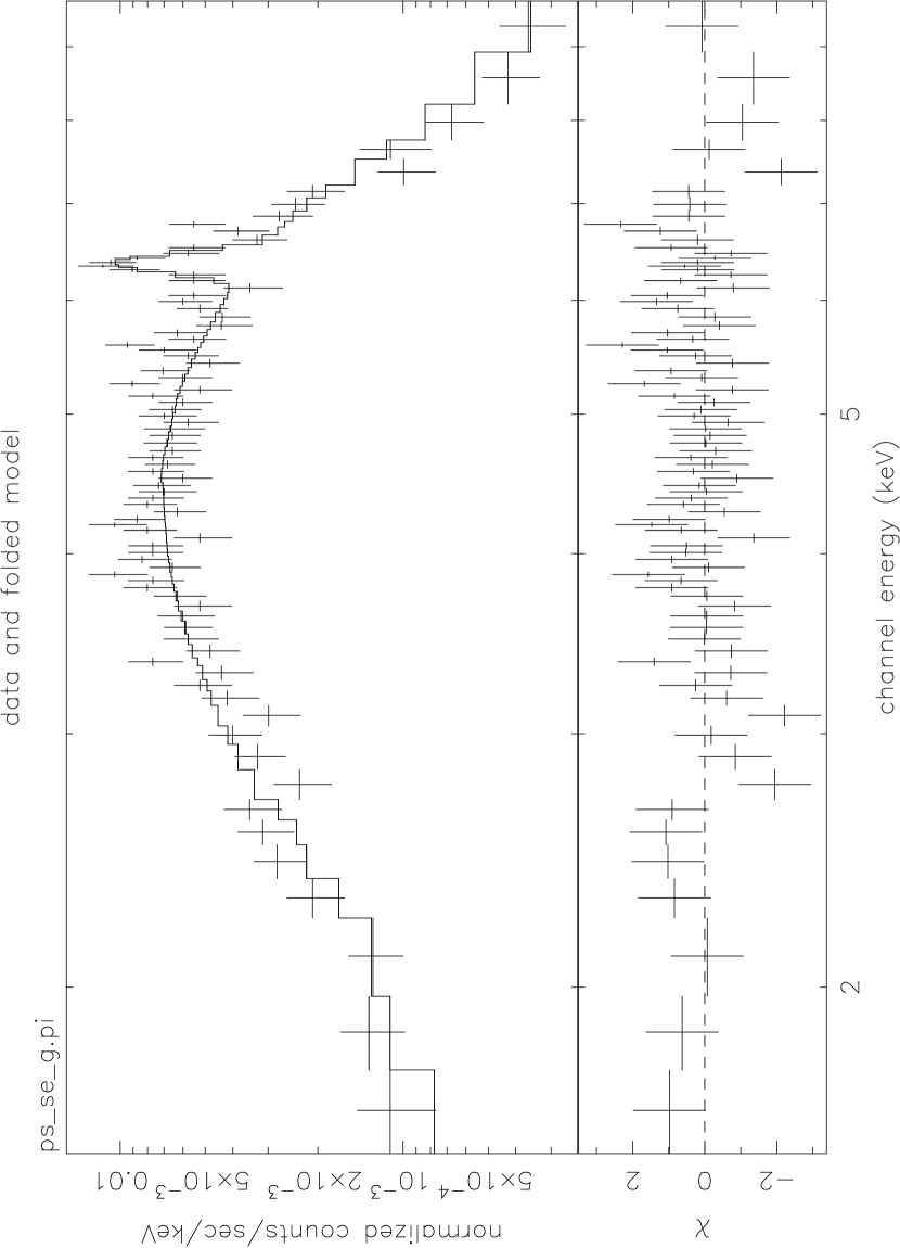
Figure 16: The spectrum and fitted model of CXO J190741.2+070650. See Table 5 for a summary of the spectral parameters.

When extracting the spectrum of CXO J190741.2+070650, we chose the background from a ring surrounding the point source. The total background-subtracted count rate from CXO J190741.2+070650 is 2.88$\times$10^-2 ct s^-1  in the 1.0–10.0 keV energy range, yielding a total of 1,922 counts. As shown in Fig. 16, the spectrum of the source is heavily absorbed, hard, and has a prominent Fe-line near 6.4 keV. Fitting the spectrum with an absorbed power law model plus a narrow Gaussian line yields an adequate fit with the parameters summarized in Table 5. The corresponding unabsorbed flux is 2.1$\times$10^-12 erg cm^-2 s^-1 in the 1–10 keV energy range.

A more detailed study of this source is beyond the scope of this paper and will be presented elsewhere. We note here that it is highly unlikely to be associated with 3C 397 due to the following reasons: 1) its location outside 3C 397 (a velocity of $\geq$1,300 km s^-1 is required for the source to be associated with the $\sim$5,000 year-old SNR at a distance of 10 kpc, see §6); 2) its high interstellar column density ($\sim$0.6$\times$10²² cm^-2 higher than that of region 11, Fig. 6); and 3) its X-ray spectrum which is unlike typical rotation-powered, accretion-powered, magnetically powered neutron stars, or cataclysmic variables. Its spectrum is however not atypical of Seyfert II Active Galactic Nuclei (AGN) which display heavily absorbed spectra with strong Fe lines. Assuming the Fe line is a red-shifted fluorescence line, the derived distance is 40$\pm$20 Mpc, and the corresponding luminosity is $\sim$4$\times$10⁴¹ erg s^-1 (at a distance of 40 Mpc).

5 Millimeter Observations

5.1 The ¹²CO observation

We first observed 3C 397 with MOPRA using six different locations along a line running from east to west and with a short integration time on each point of 3 minutes. We found an enhancement in emission on the western side at a velocity $v\sim$40 km s^-1. We subsequently pointed the SEST telescope towards the center of the SNR and made a 9$\times$9 pixel map, with 45^′′ pixel to pixel separation and a central velocity of 40 km s^-1. The antenna beam widths were 45^′′ and 22^′′ for the ¹²CO J=2–1 and J=1–0 transitions, respectively. The observations were carried out using a position beam switching mode, choosing an absolute reference position of $\alpha$ = 19^h 14^m 18^s.3 and $\delta$ = +07^o 46^′ 16^′′, J2000. Such a distant location was required to find a region without radio emission in this crowded field. The receivers yielded an overall system temperatures (including sky noise) of $\sim$340K at 230 GHz and $\sim$400K at 115 GHz, while the receiver temperatures were around 100K at 230 GHz and 10K at 115 GHz. The back end was an acousto-optical spectrometer. The low resolution spectrometer with a channel separation of 0.7 MHz (or 1.8 km s^-1 and 0.9 km s^-1 velocity resolution for the 1-0 and 2-1 transitions, respectively) was used for these observations. All the spectra intensities (antenna temperatures) were converted to the main brightness temperature scale, correcting for a main beam efficiency of 0.7 at 115 GHz and 0.5 at 230 GHz. The pointing accuracy, obtained from measurements of the SiO maser W Hya and IRAS 15194, was better than 5^′′.

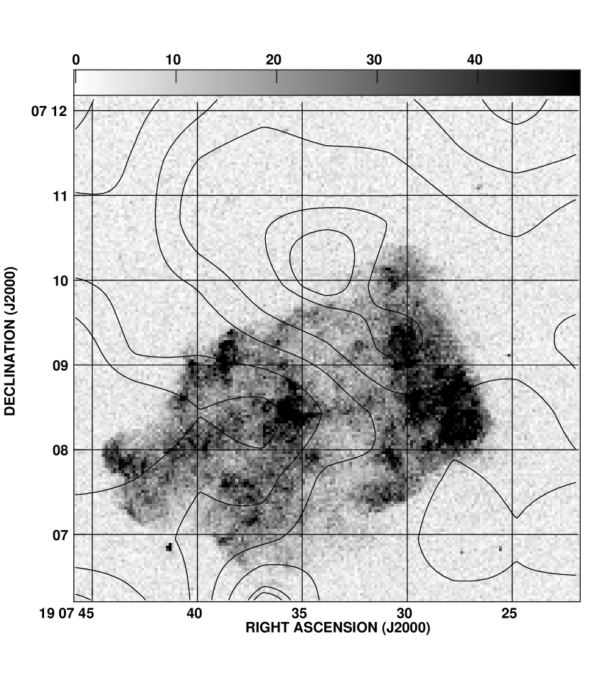
Figure 17: The ¹²CO J=1–0 and the ¹²CO J=2–1 contours obtained with SEST with the CHANDRA image overlaid. The SEST map was produced using a 9$\times$9 pixel map, with 45^′′ pixel to pixel separation and a mean velocity of 40 km s^-1. The plotted contours correspond to antenna temperatures and are: 30, 34, 38, 42, 46, 50 and 51 K for the ¹²CO J=1–0 map; and 21, 23, 25, 27, 29, 31 and 33 K for the ¹²CO J=2–1 map.

As shown in Fig. 17 and in Table 6, there is an enhancement in the molecular gas emission towards the west that is correlated with the enhanced X-ray emission. While the millimeter line emission does not seem to have the morphology of a solid flat ‘wall’, as would be expected to fit the shape of the western side of 3C 397, this gas distribution is consistent with the eastern half of the SNR being more tenuous in X-rays, since it appears to be expanding in less dense gas. A correspondence can be observed between the maximum in the ¹²CO J=1–0 emission, centered near $\alpha$ (J2000)= 19^h 07^m 34^s, $\delta$ (J2000) = 07^o 10^′ 15^′′, and a small indentation in the X-rays. In Fig. 17 (right), we show the comparison of the X-ray emission with the ¹²CO J=2–1 distribution. It shows essentially the same morphology as the ¹²CO J=1–0 transition, with a smooth gradient from west to east. Based on these correlations, we assume that the SNR 3C 397  is associated with a molecular cloud with a mean velocity of $\sim$40 km s^-1; and using the Galactic rotation curve, we derived two possible distances for 3C 397: 2.3 $\pm$0.1 kpc and 10.3$\pm$0.2 kpc for the close and far distances, respectively. The latter distance is consistent with previous distance estimates to 3C 397 (see §1).

5.2 The ¹³CO J=1–0 line transition

To confirm the association between 3C 397 and the molecular cloud found above, we examined the ¹³CO J=1–0 line transition using the IGPS data. Figure 18 displays the distribution of the ¹³CO J=1–0 line in the environs of 3C 397, for several velocity channels around $v\sim$40 km s^-1. The gas distribution is displayed in greyscale and the contours represent the CHANDRA X-ray image of 3C 397 (smoothed with a 3^′′ gaussian).

A filamentary molecular feature is noticed nearby 3C 397 between $v\sim$35.4 km s^-1 and $v\sim$ 41 km s^-1. Between $v\sim$35.4 and 36.3 km s^-1, approximately, the molecular cloud partially overlaps the SNR. From $v\geq$36.3 to $\sim$38.4 km s^-1, dense gas surrounds the western and southern (up and right sides) borders of the SNR, while the eastern extreme (bottom side in Fig. 18) expands into lower density medium, in concordance with the results shown in the ¹²CO lines (§5.1). Around $v\sim$39 km s^-1 and up to $v\sim$41.8 km s^-1, traces of an open shell around 3C 397 are apparent. In Fig. 19, we show the image in the ¹³CO J=1–0 line transition with the velocity integrated from 35.4 to 41.3 km s^-1. The apparent shell-like structure around 3C 397 could be a relic of the wind-blown bubble created by the precursor star. Higher resolution molecular and atomic observations are highly desirable to fully explore the interaction of this SNR with its surrounding interstellar gas.

6 Discussion

6.1 Distance

We now estimate the distance to the SNR using our fitted column density to the remnant. We use the range $N_{\rm H}$ = (2.9–4.3)$\times$10²² cm^-2 which encompasses the values derived for all the regions (Table 4). The extinction per unit distance in the direction of the system can be estimated from the contour diagrams given by Lucke (1978): $E_{\rm B-V}/D$ $\sim$ 1.0 mag  kpc^-1. Using the relation $<N_{\rm H}/E_{B-V}>$ = 5.55 $\times$ 10²¹ cm^-2 mag^-1 (Predehl & Schmitt 1995), we derive a distance of 5.2–7.8 kpc. This distance is smaller that that derived from the millimeter observations (10.1–10.5 kpc), but not inconsistent with the range (6.4–12.8 kpc) determined from HI absorption studies. We will subsequently scale our calculations to the parameter $D_{10}=D/10$ kpc, and keep in mind that $D_{10}$ could span the range 0.6–1.3.

6.2 A compact stellar remnant and the nature of the hot spot

We found two point sources in the CHANDRA field: a soft source at the north-eastern edge, and a hard source just outside the south-eastern edge. As discussed in §3 and §4.4, we believe that none of these sources is associated with the SNR.

The hot spot was proposed to be the compact stellar remnant or a mini-plerion. Our imaging and spectral analysis has confirmed that the hot spot can not be either. We can not however rule out the presence of a compact object buried underneath the thermal emission with an unabsorbed flux of $\leq$ 6$\times$10^-13 erg cm^-2 s^-1, which translates to a luminosity of $L_{x}$ (0.5–10 keV) = 7$\times$10³³ $D_{10}^{2}$ erg s^-1.

As to the origin of the hot spot, we suggested in §4.2.1 that it could be a clump arising from a shocked cloudlet. To estimate the corresponding density, we use the vpshock model parameters summarized in Table 2. The observed measured emission measure of the soft component ($EM_{s}$) of 0.108 corresponds to $\int n_{e}n_{\rm H}dV$ $\sim$ $f_{s}n_{e}n_{\rm H}V=10^{14}(4\pi D^{2})(EM)$ = 1.3$\times$10⁵⁹ cm^-3; where $f_{s}$ is the volume filling factor of the soft component, $n_{e}$ is the post-shock electron density, and $n_{\rm H}$ $\sim$ $n_{e}$/1.2. Using a radius of 12^′′.5 for the hot spot, we estimate $n_{e}$ = 72 $f_{s}^{-1/2}$ cm^-3, implying an upstream ambient density $n_{0}$ = $n_{e}/4.8$ = 15 $f_{s}^{-1/2}$cm^-3 (for cosmic abundance plasma and the strong shock Rankine-Hugoniot jump conditions; $n_{0}$ here includes only hydrogen). This corresponds to $n_{0}$$\sim$15–50 cm^-3 for filling factors $f_{s}$$\sim$0.1–1.0.

6.3 Origin of the soft and hard components

In the following, we discuss the origin of the soft and hard components; using our two-component model fits (§4.2). We again remind the reader that a two-temperature component model is likely to be an oversimplified model for this complex SNR (§4.3), so considerable caution is required in interpreting the two-component model fits. The parameters derived from our two-component fits nevertheless describe the global spectral differences across the SNR.

In our ASCA study we suggested two scenarios for the interpretation of the two-component global fit. For the 2 kyr-old ejecta-dominated SNR, the soft component would arise from reverse-shocked ejecta and the hard component from the blast wave shocking an ambient medium with a density of $n_{0}$$\sim$ 1.0 $D_{10}^{-1/2}$ cm^-3. For the 5 kyr-old SNR propagating in a dense medium, the soft component would correspond the blast wave propagating in a medium of density $n_{0}$$\sim$33 $D_{10}^{-1/2}$ cm^-3. In the first scenario, one expects the hot component to originate from the SNR ‘shell’ and to be characterized by solar (or sub-solar abundances); while the soft component should be located inside the SNR ‘shell’ and characterized by above-solar abundances. For the second scenario, one expects the opposite behavior. Furthermore, the ionization timescales should decrease with radius for the blast wave component (forward shock) since the interior is shocked first, and to increase with radius for the ejecta component (reverse-shock).

Morphologically, the CHANDRA energy color image (Fig. 1) shows that the softest X-ray emission is found near the edge of the eastern lobe and the south-eastern boundary, and that the hard component (while visible in most regions) is more concentrated inside the SNR (see also Figs 5, 8, 9). Furthermore, our spectroscopic study shows that the ionization timescales have a general trend to decrease outwards for the soft component and to increase outwards for the hard component (except for the regions inside the low-surface brightness ‘strip’, see Figs 8 and 9). This, together with the high Fe abundances required to fit the hard component, support the second scenario where the SNR is propagating in a dense medium. Using our vpshock fit to the soft component (Tables 2-4) and following the calculations done above for the hot spot (§6.2), we estimate pre-shocked ambient densities ranging from $n_{0}$$\sim$15–70 $(f_{s}D_{10})^{-1/2}$ cm^-3, a range that brackets the average density derived from our global ASCA fit for large filling factors, $f_{s}$.

For the hard component, the derived high Fe abundances, relatively low ionization timescales and emission measures support the presence of reverse-shocked Fe bubbles. Using our vpshock fits to the hard component (Tables 2-4), we estimate pre-shocked electron densities, $n_{e}$, ranging from 1.5–8 $(f_{h}D_{10})^{-1/2}$ cm^-3 which then imply that the hot plasma has been shocked at a time $t$=$\tau_{h}$/$n_{e}$$\sim$700–4,000 $(f_{h}D_{10})^{1/2}$ years ago. The volume filling factor, $f_{h}$, can not be accurately determined due to the poor signal to noise ratio in the hard energy band. For a filling factor $f_{h}$$\sim$0.1–1.0, we estimate $n_{e}$$\sim$1.5–25 cm^-3 and $t$$\sim$220–4,000 years; a reasonable timescale for a reverse shock to develop in a $\sim$5,300 year-old SNR. Regions 7, 8, and 9 are an exception: the soft and hard component’s ionization timescales are different from the other regions. This, together with their low-surface radio and X-ray brightness, suggest that the conditions in this region are different from elsewhere in the SNR. Furthermore, the much lower ionization timescales of the soft component (Table 4) indicate that the cool plasma has been just recently shocked in these regions. We speculate that this is due to a reflected shock, perhaps from encountering a nearby molecular cloud. Since the spectral parameters are poorly constrained, a better understanding of the ambient conditions and a theoretical investigation of the SNR dynamics has to await future X-ray observations.

6.4 Classification of 3C 397: Interaction with a cloud?

As we mentioned above, our ¹²CO and ¹³CO study shows that the ambient medium is more tenuous in the eastern lobe, and indicates the presence of a molecular cloud near $\sim$40 km s^-1. The peculiar rectangular morphology, the sharp western boundary, the enhanced radio, millimeter, and X-ray emission and the higher column density in the west support the scenario where 3C 397 is expanding in an inhomogeneous medium, being denser in the west; and likely encountering or interacting with the molecular cloud. While the absolute value of $N_{\rm H}$ is model dependent, the difference in $N_{\rm H}$ between the east and west is not (Tables 1-4). If the difference of $\sim$(0.5–1.0)$\times$10²² cm^-2 is solely due to a density gradient caused by a molecular cloud, then the corresponding average density would be $\sim$ 160–320  ($\delta$$l_{10~{}pc}$)^-1 $D_{10}^{-1}$ cm^-3; where we have assumed that the line of depth of the SNR in the cloud, $\delta$$l$, is close to the average SNR size of 10 pc.

3C 397 bears resemblance to mixed-morphology SNRs like 3C 391 (Chen & Slane 2001) and CTB 109 (Rho & Petre 1997) because of the following: 1) it has a centrally filled X-ray morphology dominated by thermal emission; 2) it has a ‘shell’-like radio morphology, and 3) it displays asymmetries in the overall X-ray morphology and variations in the distribution of $N_{\rm H}$ across the remnant which have been attributed to the presence of dense material that the remnant is encountering. In mixed-morphology SNRs, the derived abundances from X-ray spectra are however more or less consistent with solar values, indicating that their enhanced X-ray emission is due to either evaporation of engulfed cloudlets or a radiative stage of evolution in which thermal conduction plays an important role.

For 3C 397 however, the X-ray spectrum is more complex because of: a) the need for a two-component model everywhere in the remnant and in arcseconds-scale regions, b) the enhanced metal abundances indicating an ejecta origin, and c) the presence of an outer X-ray ‘shell’ which is strongly correlated with the radio ‘shell’. We note here however that this outer edge has a geometry that is more rectangular than spherical and that some parts of the remnant’s limb are missing. Furthermore, even the outermost western boundary (region 12) hints at the presence of shocked ejecta Fe indicating that the reverse shock did penetrate to large radii (Table 4). This could occur in the presence of vigorous turbulence caused by the presence of Fe bubbles. Three-dimensional hydrodynamical simulations by Blondin et al. (2001) show that in this case, the Fe bubbles will be mixed with other heavy elements and with the ambient normal abundance gas. Furthermore, turbulence will affect the morphology of the SNR by creating ‘jet’-like features resulting from the interaction of bubbly ejecta with the ambient medium, and by enhancing the radio synchrotron emissivity in strong turbulent regions.

While the above properties indicate that 3C 397 is unlike the ‘classical’ mixed-morphology SNRs, the differences can be explained if we take into account the relative youth of 3C 397  compared to the other SNRs in which the signature of ejecta has been wiped out due to a later evolutionary stage in the SNR lifetime. An SNR enters the radiative pressure-driven snowplow phase (PDS) when its radius is: $r_{PDS}$ = 14 $E_{51}^{2/7}$ $n_{0}^{-3/7}$ (pc). Using an explosion energy $E_{51}$$\sim$1.2 $D_{10}^{5/2}$ and an average ambient density $n_{0}$$\sim$33 $D_{10}^{-1/2}$ (Safi-Harb et al. 2000), we estimate a radius $r_{PDS}$$\sim$3.3 pc which is comparable to the size of the remnant ($R$$\sim$3.5-7 pc). This implies that 3C 397 must be entering into its PDS phase; and so we speculate that it will eventually resemble the mixed-morphology SNRs.

It is currently believed that the excitation of the hydroxyl radical 1720 MHz maser is a good indicator of interaction between SNRs with dense molecular environments. Evidence that mixed-morphology SNRs produce OH masers has been recently accumulating (e.g. Yusef-Zadeh et al. 2003). To search for maser emission from 3C 397, we have observed it at 1720 MHz with the VLA on 2003 May 16 (W. M. Goss, private communication). The beam was 50^′′ by 35^′′, the rms noise about 7 mJy/beam (comparable to the sensitivity achieved in other searches; W. M. Goss, private communication) and the velocity resolution of about 1.2 km/s over 127 channels. No lines were found. However, this does not necessarily imply the absence of interaction with a molecular cloud, but could rather indicate that the critical conditions required to excite OH masers are not yet achieved (Green et al. 1997). Similarly, we find that the ¹²CO 2-1/1-0 ratio (after converting the antenna temperature into brightness temperature) is quite homogeneous throughout the field, and about 0.87. Thus, this is not a very strong indication that some specific cloud is being shocked, as the expected ratio for shocked gas is $\geq$1. In conclusion, the lack of OH masers and the small ratio of CO 2–1/1–0 ($<$ 1) could indicate that the molecular cloud in the close vicinity has not yet been overrun by the shock wave. Alternatively, if the shock/cloud interaction is occurring in 3C 397, it must be taking place along the line of sight. This latter model provides an explanation to the X-ray shocked material and the lack of OH (1720 MHz) masers, because these masers are mainly excited when the shock front is almost transverse to the line of sight (Wardle 1999).

A high-resolution study of the molecular and atomic gas in the environs are needed to better probe the level of excitation of the adjoining molecular cloud.

7 Conclusions

We have presented a CHANDRA ACIS-S3 observation of the SNR 3C 397. Previous studies of this SNR have shown that the remnant has a double-lobed elongated morphology with enhanced X-ray emission from the center and the western lobe. Most intriguing is a central enhancement of X-ray emission seen with ROSAT and suggestive of a compact X-ray source or a PWN associated with 3C 397. The spectrum of this ‘hot spot’ could not be resolved with previous X-ray missions and left the classification of 3C 397 uncertain. CHANDRA’s imaging capabilities allowed us to resolve the emission from the hot spot. We confirm its thermal nature, thus ruling out a PWN or a central compact object. We put an upper limit on the luminosity of a buried compact object $L_{x}$ (0.5–10 keV) $\leq$ 7$\times$10³³ erg s^-1 at an assumed distance of 10 kpc. In addition, we discovered a hard point-source, CXO J190741.2+070650, located outside and southeast of the SNR. The properties of this source lead us to believe that it is not associated with 3C 397, and that it is most likely a nearby AGN.

The CHANDRA images reveal the softest X-ray emission from a plume-like structure at the edge of the eastern lobe and in the southeast, arcseconds-scale clumps and knots most notably in the western lobe, jet-like structures running along the symmetry axis of the SNR, a low-surface brightness diffuse emission between the hot spot and the western lobe, and a sharp western boundary which is almost rectangular in the southwest. Except for the central ‘hot spot’, the clumps and knots seen in the broadband X-ray image are strongly correlated with the radio VLA image. The line-free 4–6 keV X-ray emission appears however to be contained within the radio shell.

Our spatially resolved spectroscopic study of the small scale regions shows that one-component models are inadequate, and that at least two NEI thermal components are needed to fit the spectra of each region. In particular, we find that:

• For the hot spot, the soft component has reached ionization equilibrium and is characterized by $kT_{s}$$\sim$0.18$\pm$0.3 keV and solar abundances. The hot component is far from ionization equilibrium and is characterized by $kT_{h}$$\sim$2.5${}^{+1.0}_{-1.4}$ keV and an enhanced S abundance ($\geq$3.0 at the 2$\sigma$ level). We interpret the hot spot as a shocked cloudlet with a pre-shocked density $\sim$15–50 cm^-3 and possibly mixed with hot S ejecta.

• For the eastern and western lobes, our two-component vpshock fits require enhanced abundances in both the soft and hard components; in particular a high Fe abundance ($\geq$9 $\odot$) is needed to account for the strong Fe-K lines at 6.5 keV. This indicates that the hard component is at least partially due to shock-heated Fe ejecta. The column density and the brightness are higher in the west indicating a denser medium on the western side.

• For the small scale regions, we find that two-component vpshock models yield adequate fits, with a general trend of increase of $N_{\rm H}$ from east to west. The soft component’s temperature varies from $\sim$0.15 keV in the eastern and southeastern edge to $\sim$0.26 keV in the low-surface brightness interior. The hard component’s parameters are less constrained but the temperature is $\sim$1–3 keV and possibly higher along the eastern ‘jet’-like structure. The ionization timescales of the soft component are generally higher than those of the hard component. Furthermore, the abundances of the soft component are generally consistent with solar (except for some regions) while those of the hard component generally require above-solar S and Fe abundances. We interpret this as evidence for a combination of a multi-temperature ejecta and shocked ambient/cicumstellar material. The enhanced Fe abundances in the outermost regions of the remnant indicate that the ejecta have penetrated to large radii as would be expected from enhanced turbulence caused by shocked Fe bubbles.

The quality of the data does not allow us to constrain the parameters of the hard component. While we do not find compelling evidence for hard non-thermal emission from 3C 397, we put an upper limit on the luminosity of the hard line-free emission in the 4–6 keV of $L_{x}$ (4–6 keV)$\leq$1.3$\times$10³³ $D_{10}^{2}$ erg s^-1.

The overall imaging and spectral properties of 3C 397 favor the interpretation of the SNR being a $\sim$5,300 year-old SNR propagating in a dense medium, and likely encountering a molecular cloud in the west. This conclusion is supported by our millimeter observations with SEST and the IGPS database where the line emission in the ¹²CO and ¹³CO (J=1–0) transitions show an enhancement of brightness on the western side, correlated with the X-ray brightness and peaking near $v\sim$38–40 km s^-1. The derived distance of 10 kpc agrees with previous estimates and strengthens the association between 3C 397 and the molecular cloud. Finally, we conclude that 3C 397 is at the critical stage of entering into its radiative phase; and propose that it will eventually evolve into the more classical mixed-morphology SNRs.

Table 1: Spectral results for the eastern lobe, the central ‘hot spot’, and the western lobe. The model used was a two-component thermal bremsstrahlung with Gaussian lines, modified by interstellar absorption with column density $N_{\rm H}$.

Parameter/Region	east	west	hot spot
NH (1022 cm-2)	2.27 (2.24-2.31)	2.86 (2.84-2.89)	2.76 (2.6-3.6)
kTs (keV)	0.25 (0.239-0.251)	0.256 (0.25-0.26)	0.21 (0.17-0.25)
EMsa	1.34 (1.24-1.76)	3.97 (3.96-4.1)	0.9 (0.15-6.7)
kTh (keV)	3.4 (3.0-4.1)	2.87 (2.58-3.33)	1.5 (0.93-3.3)
EMha ($\times$10-4)	5.3 (4.5-6.2)	13.3 (11.6-13.5)	1.8 (0.5–5.6)
E1 (Ne-Ly$\alpha$, Fe-L blend)	0.99 (0.95-1.0)	1.0 (0.999-1.01)
E2 (Mg He$\alpha$)	1.33 (1.32-1.34)	1.345 (1.33-1.35)
E3 (Si He$\alpha$)	1.825 (1.816-1.830)	1.825 (1.815-1.828)	1.79 (1.74-1.84)
E4 (S He$\alpha$)	2.415 (2.41-2.42)	2.418 (2.415-2.423)	2.41 (2.38-2.44)
E5 (S He$\beta$?)	2.90 (2.83-2.95)	2.931 (2.907-2.950)	2.87 (2.84-2.90)
E6 (Ar He$\alpha$)	3.12 (3.09-3.15)	3.1 (3.08–3.11)
E7 (Ca He$\alpha$)		3.826 (3.79-3.86)
E8 (Fe He$\alpha$)	6.498 (6.48-6.51)	6.546 (6.53-6.56)
Fluxua (0.5-8 keV), soft	1.7$\times$10-10	5.30$\times$10-10	6.3$\times$10-11
Fluxua (0.5-8 keV), hard	1.7$\times$10-12	3.0$\times$10-12	3.4$\times$10-13
$\chi^{2}_{\nu}$ ($\nu$)	1.75 (219)	1.88 (265)	0.87 (116)
cts s-1 arcsec-2	8.04$\times$10-5	1.33$\times$10-4	2.34$\times$10-4

^a the emission measure in units of (3.02$\times$10^-15/4$\pi$$D^{2}$)$\int$$n_{e}$$n_{i}$$dV$ cm^-5, where $n_{e}$ and $n_{i}$ are the electron and ion densities in cm^-3, respectively.

Table 2: Two-component thermal model for the hot spot. Errors are at the 2$\sigma$ level.

Parameter	vpshock+vpshock	vpshock+mekal
$N_{\rm H}$ (1022 cm-2)	2.94 (2.9–3.5)	3.26 (3.0–3.4)
$kT_{s}$ (keV)	0.19 (0.15–0.20)	0.18 (0.15–0.21)
$\tau_{s}$ (1013 cm-3 s)	3.5	–
$kT_{h}$ (keV)	2.7 (1.3–3.7)	2.5 (1.4–7.6)
$\tau_{h}$ (1010 cm-3 s)	6.5 (3.6–42)	4.1 (1.9–56)
Sa	5 (3–18)	6.9 (3-15)
$\chi^{2}_{\nu}$	0.96 (119)	1.0 (120)

^a The abundances of all other elements are consistent with solar.

Table 3: The spectral fitting results of the eastern and western lobes. The model used was a two-component vpshock model, modified by interstellar absorption. The abundances (in solar units) of the soft component were tied to those of the hard component (except for the Fe abundance of the hot component). A Gaussian line near 3.1 keV has been added to account for the emission from Argon. Errors are at the 3$\sigma$ level and were determined after freezing the parameters of the second component to their best fit values.

Parameter	eastern lobe	western lobe
$N_{\rm H}$ (1022 cm-2)	2.85 (2.7–2.9)	3.27 (3.1–3.5)
$kT_{s}$ (keV)	0.20 (0.195–0.215)	0.215 (0.20–0.23)
$\tau_{s}$ (1011 cm-3 s)	1.6 (1.3–2.1)	1.2 (0.75–1.9)
$norm_{s}$a	4 (3–5.4)	3.3 (2.0–5.5)
$kT_{h}$ (keV)	1.6 (1.5–2.2)	1.4 (1.3–1.6)
$\tau_{h}$ (1011 cm-3 s)	1.4 (1.0–2.0)	2.7 (1.9–4.0)
$norm_{h}$a	2.7 (2.3–3.1) $\times$10-3	4.9 (4–6) $\times$10-3
O	1.5 (1.1–1.7)	7.4 (4.5–11.5)
Ne	0.38 ($\leq$0.5)	1.1 (0.4–2.2)
Mg	0.1 ($\leq$0.2)	0.46 (0.3–0.65)
Si	0.5 (0.45–0.65)	1.0 (0.8–1.3)
S	1.9 (1.7–2.2)	3.3 (2.8–4.0)
Ca	1.4 ($\leq$4)	3.1 (1–6)
Feh	12 (9–14)	15 (12–20)
$\chi^{2}_{\nu}$	2.1 (226)	2.25 (277)

^a the normalization in units of (10^-14/4$\pi$$D^{2}$)$\int$$n_{e}$$n_{\rm H}$$dV$ cm^-5, where $D$ is the distance to the source (cm), $n_{e}$ and $n_{\rm H}$ are the electron and hydrogen densities in cm^-3, respectively.

Table 4: Spectral Parameters of the small regions shown in Fig. 6. The model used is a two-component $\it{vpshock}$ model. The errorbars are large. The 2$\sigma$ errors shown below are determined after freezing all the other parameters to their best-fit values. See text for details.

Region	$N_{\rm H}$	$kT_{s}$	$tau_{s}$	$kT_{h}$	$tau_{h}$	S	Fe	$\chi^{2}_{\nu}$ ($\nu$)
	(1022 cm-2)	(keV)	(1012 cm-3 s)	(keV)	(1011 cm-3 s)	solar	solar
1	3.03${}^{+0.12}_{-0.03}$	0.15	1.05${}^{+0.55}_{-0.45}$	1.4${}^{+0.35}_{-0.25}$	3.5${}^{+7.5}_{-1.5}$	2.8${}^{+2.2}_{-0.8}$	10($\geq$5)	1.86 (97)
2	2.86${}^{+0.04}_{-0.26}$	0.16	1.7$\geq$2	1.7${}^{+0.4}_{-0.35}$	1.7${}^{+2.3}_{-0.2}$	2.0${}^{+1.6}_{-0.8}$	6${}^{+8}_{-3}$	1.59 (90)
3	2.95${}^{+0.15}_{-0.05}$	0.23	49($\geq$6)	18$\geq$8	0.48${}^{+0.22}_{-0.13}$	5.2$\pm$1.2	2.1${}^{+0.7}_{-0.3}$	1.8 (124)
4	3.43${}^{+0.11}_{-0.09}$	0.18	46($\geq$6)	2.4${}^{+0.9}_{-0.4}$	0.32${}^{+0.18}_{-0.08}$	3.3${}^{+1.2}_{-0.8}$	1.5${}^{+1.3}_{-1.4}$	1.63 (112)
5	3.67${}^{+0.13}_{-0.12}$	0.19	2.23${}^{+7.8}_{-1.7}$	1.53${}^{+0.19}_{-0.07}$	2.1${}^{+0.6}_{-1.96}$	2.4${}^{+0.3}_{-0.4}$	6.3${}^{+1.0}_{-1.7}$	1.4 (189)
6	3.96${}^{+0.02}_{-0.08}$	0.17	0.5${}^{+0.07}_{-0.03}$	1.58${}^{+0.12}_{-0.28}$	2.0${}^{+3}_{-0.5}$	1.8${}^{+0.5}_{-0.6}$	5.2($\geq$3.5)	2.3 (204)
7	3.0${}^{+0.21}_{-0.19}$	0.26	0.05${}^{+0.03}_{-0.025}$	1.0${}^{+0.14}_{-0.06}$	6${}^{+12}_{-2}$	0.6${}^{+0.3}_{-0.1}$	1.4${}^{+0.5}_{-0.7}$	1.14 (129)
8	3.2${}^{+0.3}_{-0.2}$	0.26	0.007${}^{+0.003}_{-0.002}$	2.4${}^{+1.0}_{-0.8}$	2.4${}^{+9.6}_{-0.4}$	8($\geq$3)	14$\pm$5	1.0 (70)
9	3.85${}^{+0.25}_{-0.15}$	0.22	0.030${}^{+0.022}_{-0.010}$	1.04${}^{+0.11}_{-0.09}$	12.5($\geq$0.5)	1.5${}^{+0.9}_{-0.4}$	7${}^{+6}_{-3}$	1.19 (115)
10	3.36${}^{+0.24}_{-0.06}$	0.23	26($\geq$2)	3.4${}^{+1.5}_{-0.9}$	0.7${}^{+0.5}_{-0.2}$	3.5${}^{+1.5}_{-1.2}$	5.2${}^{+2.3}_{-1.7}$	1.1 (107)
11	3.6${}^{+0.12}_{-0.01}$	0.17	0.32${}^{+0.18}_{-0.02}$	1.38${}^{+0.32}_{-0.13}$	2.6${}^{+2.4}_{-1.1}$	1.9${}^{+1.6}_{-0.4}$	4.6${}^{+2.4}_{-2.1}$	1.49 (139)
12	4.10${}^{+0.16}_{-0.14}$	0.19	0.27${}^{+0.27}_{-0.12}$	1.03${}^{+0.21}_{-0.13}$	5.3($\geq$2.0)	2.0${}^{+0.7}_{-0.6}$	10${}^{+8}_{-3}$	1.23 (118)

Table 5: Spectral parameters of hard point source south-east of 3C 397. The model is an absorbed power law with a Gaussian line. Errors are at the 2$\sigma$ level.

$N_{\rm H}$ (1022 cm-2)	5.5 (4.4-6.7)
$\Gamma$	0.025 (-0.22–0.28)
$norm.$	2.7 (1.7–4.2) $\times$10-5
$E_{0}$	6.345 (6.32–6.37)
$EQW$	425 eV
$norm.$	1.08 (0.8–1.3) $\times$10-5
$\chi_{\nu}^{2}$	0.85
$\nu$	79
$F_{observed}$ (1–10 keV)	1.75$\times$10-12 erg cm-2 s-1
$F_{ua}$ (1–10 keV)	2.1$\times$10-12 erg cm-2 s-1

Table 6: Millimeter Line Flux density in 3C 397. See §5 for details.

Location	Antenna Temp.	Antenna Temp.	Line Flux Density	Line Flux Density
	12CO J=1-0	12CO J=2-1	12CO J=1-0	12CO J=2-1
	(K)	(K)	(Jy)	(Jy)
Center	3.7	2.3	1.43	1.24
North	2.81	1.56	1.08	0.84
South	3.82	2.08	1.47	1.12
East	2.49	1.5	0.96	0.52
West	4.79	2.72	1.85	1.00

Figure 1: The energy image of 3C 397. Red, green, and blue correspond to the 0.5–1.5 keV, 1.5–2.5 keV, and 2.5–8 keV ranges, respectively. The individual images have been adaptively smoothed using a Gaussian kernel and an FFT algorithm, with a minimum (maximum) smoothing scale of 2 (4) pixels, and with a minimal (maximal) signal to noise ratio of 3 (5).

Figure 2: The CHANDRA S3 smoothed images of the central X-ray spot (left) and the hard point-source southeast of 3C 397 (right). Both images are shown on the same scale.

Figure 3: The CHANDRA image in the 0.5–2.4 keV band, with the ROSAT HRI contours overlayed. The CHANDRA image has been smoothed with the ciao tool $csmooth$ using a tophat filter with 2^′′ (5^′′) minimum (maximum) scale and a minimum significance of 3$\sigma$. The HRI image has been smoothed with a Gaussian with sigma=4^′′ to show the enhanced emission from the central spot centered at $\alpha$=19^h 07^m 35^s.13, $\delta$=07^o 08^′ 28^′′.76 (J2000). The arrows point to the soft and hard point sources discussed in §3 and §4.4.

Figure 4: The CHANDRA 0.3–10 keV image with the VLA L-band contours overlayed.

Figure 5: The CHANDRA 4 to 6 keV image (color) with the radio VLA L-band contours overlayed.

Figure 6: The regions selected for spatially resolved spectroscopy (§4).

Figure 7: The distribution of the column density, $N_{\rm H}$, expressed in units of 10²² cm^-2. $N_{\rm H}$ was derived using the two-component vpshock models summarized in Table 4. Note that the image contrast has been suppressed to display the numbers.

Figure 8: The distribution of the soft component’s temperature (expressed in keV, left) and ionization timescale (in units of 10¹² cm^-3 s^-1, right). See Table 4 and §4.2 for details.

Figure 9: The distribution of the hard component’s temperature (expressed in keV, left) and ionization timescale (in units of 10¹¹ cm^-3 s^-1, right). See Table 4 and §4.2 for details.

Figure 10: The data (crosses) and the fitted model for the central ’hot spot’ in 3C 397. The model used is a two-component vpshock model. The components of the model are shown as dashed lines. The bottom panel displays the residuals in units of sigmas. The parameters of the fits are summarized in Table 2.

Figure 11: The data (crosses) and the fitted model for the eastern (left) and western (right) lobes of 3C 397. The model used is a two-component vpshock model. A Gaussian line has been added to account for the line emission from Argon. The components of the model are shown as dashed lines. The bottom panel displays the residuals in units of sigmas. The parameters of the fits are summarized in Table 3. Both plots are shown on the same y-scale.

Figure 12: The soft north-eastern plume (region 1 located in the eastern lobe) and the north-western knot (region 5 located in the western lobe) fitted with a two-component vpshock model. A Gaussian line has been added to account for the line emission from Argon. The parameters of the model are summarized in Table 4. See §4 for details.

Figure 13: The eastern (left) and western (right) jet-like features (regions 3 and 4) fitted with a two-component vpshock model. A Gaussian line has been added to account for the line emission from Argon. The parameters of the fits are summarized in Table 4. Both plots are shown on the same y-scale.

Figure 14: The spectra of the low-surface brightness regions northwest and southwest of the hot spot (regions 7 and 9), fitted with a two-component vpshock model. A Gaussian line has been added to account for the line emission from Argon. The parameters of the fits are summarized in Table 4.

Figure 15: The spectra of the northeastern and southeastern clumps (regions 10 and 11), fitted with a two-component vpshock. A Gaussian line has been added to account for the line emission from Argon. The parameters of the fits are summarized in Table 4.

Figure 18: The ¹³CO J=1–0 images in the environs of 3C 397, as taken form the International Galactic Plane Survey (IGPS) for several velocity channels around $v\sim$40 km s^-1. The gas distribution is displayed in greyscale. The contours represent the CHANDRA X-ray image of 3C 397 (smoothed with a 3^′′ gaussian).

Figure 19: The ¹³CO J=1–0 image of 3C 397 obtained with the IGPS and integrated between 35.4 and 41.3 km s^-1. The CO distribution is shown in greyscale and the contours outline the CHANDRA X-ray emission from 3C 397.

References

- (1) Anderson, M. C., & Rudnick, L. 1993, ApJ, 408, 514
- (2) Becker, R. H., Markert, T., & Donahue, M. 1985, ApJ, 296, 461
- (3) Borkowski, K. J., Lyerly, W. J., & Reynolds, S. P. 2001, ApJ, 548, 820
- (4) Blondin, J. M., Borkowski, K. J., & Reynolds, S. P. 2001, ApJ, 557, 782
- (5) Caswell, J. L., Murray, J. D., Roger, R. S., Cole, D. J., & Cooke, D. J. 1975, A&A, 45, 239
- (6) Cersosimo, J. C., & Magnani, L. 1990, A&A, 239, 287
- (7) Chen, Y., Sun, M., Wang, Z.-R., & Yin, Q. F. 1999, ApJ, 520, 737
- (8) Chen, Y. & Slane, P. O. 2001, ApJ, 563, 202
- (9) Dyer, K. K., & Reynolds, S. P. 1999, ApJ, 526, 365
- (10) Gooch, R. E. 1996, Pub. Astron. Soc. Aus., 14, 106
- (11) Green, A. J., Frail, D. A., Goss, W. M., & Otrupcek, R. 1997, ApJ, 114, 2058
- (12) Green, D.A. 2004, A Catalogue of Galactic Supernova Remnants (Cambridge MRAO, Cavendish Laboratory)
- (13) Kassim, N. 1989, ApJS, 71, 799
- (14) Keohane, J. W., Foster, A., Vu, I., & Olbert, C. M. 2003, American Astronomical Society’s High-Energy Astrophysics Division Meeting, #35, #10.25
- (15) Liedahl, D. A., Kahn, S. M., Osterheld, A. L., & Goldstein, W. H. 1990, ApJ, 350, L37
- (16) Lucke, P. B. 1978, A&A, 64, 367
- (17) Mewe, R., Gronenschild, E. H. B. M., & van den Oord, G. H. J. 1985, A&AS, 62, 197
- (18) Predehl, P. & Schmitt, J. H. M. M. 1995, A&A, 293, 889
- (19) Rho, J. 1995, Ph.D. thesis, Univ. of Maryland
- (20) Rho, J., & Petre, R. 1997, ApJ, 484, 828
- (21) Rho, J., & Petre, R. 1998, ApJ, 503, L167
- (22) Rozyczka M., Tenorio-Tagle, G., Franco, J. & Bodenheimer, P. 1993, MNRAS, 261, 674
- (23) Safi-Harb, S., Petre, R., Arnaud, K. A., Keohane, J. W., Borkowski, K. J., Dyer, K. K., Reynolds, S. P., & Hughes, J. P. 2000, ApJ, 545, 922
- (24) Townsley, L. K., Broos, P. S., Garmire, G. P., & Nousek, J. A. 2000, ApJ, 534, L139
- (25) Yusef-Zadeh, F., Wardle, M., Rho, J., & Sakano, M. 2003, ApJ, 585, 319
- (26) Wardle, M. 1999, ApJ, 525, L101