The Crab Nebula and Pulsar between 500 GeV and 80 TeV: Observations with the HEGRA stereoscopic air Cherenkov telescopes

Abstract

The Crab supernova remnant has been observed regularly with the stereoscopic system of 5 imaging air Cherenkov telescopes that was part of the High Energy Gamma Ray Astronomy (HEGRA) experiment. In total, close to 400 hours of useful data have been collected from 1997 until 2002. The differential energy spectrum of the combined data-set can be approximated by a power-law type energy spectrum: $d\Phi/dE=\Phi_{0}\cdot(E/\mathrm{TeV})^{\Gamma}$, $\Phi_{0}=(2.83\pm 0.04_{\mathrm{stat}}\pm 0.6_{\mathrm{sys}})$ $\cdot 10^{-11}$ ph cm^-2 s^-1 TeV^-1 and $\Gamma=-2.62\pm 0.02_{\mathrm{stat.}}\pm{0.05}_{\mathrm{sys.}}$. The spectrum extends up to energies of 80 TeV and is well matched by model calculations in the framework of inverse Compton scattering of various seed photons in the nebula including for the first time a recently detected compact emission region at mm-wavelengths. The observed indications for a gradual steepening of the energy spectrum in data is expected in the inverse Compton emission model. The average magnetic field in the emitting volume is determined to be $(161.6\pm 0.8_{\mathrm{stat}}\pm 18_{\mathrm{sys}})~{}\mu$G. The presence of protons in the nebula is not required to explain the observed flux and upper limits on the injected power of protons are calculated being as low as 20 % of the total spin down luminosity for bulk Lorentz factors of the wind in the range of $10^{4}-10^{6}$. The position and size of the emission region have been studied over a wide range of energies. The position is shifted by 13^′′ to the west of the pulsar with a systematic uncertainty of 25^′′. No significant shift in the position with energy is observed. The size of the emission region is constrained to be less than 2^′ at energies between 1 and 10 TeV. Above 30 TeV the size is constrained to be less than 3^′. No indications for pulsed emission has been found and upper limits in differential bins of energy have been calculated reaching typically 1-3 % of the unpulsed component.

1 Introduction

Observations of the Crab pulsar and nebula have been carried out in every accessible wavelength band (ground and space based). The source has been established as a TeV emitter with the advent of ground based Cherenkov imaging telescopes with sufficient sensitivity (Weekes et al., 1989). The broad band spectral energy distribution (SED) is exceptionally complete in coverage and unique amongst all astronomical objects observed and studied. The historical lightcurve of the supernova explosion of 1054 A.D. is not conclusive with respect to the type of progenitor star and leaves many questions concerning the stellar evolution of the progenitor star unanswered (Stephenson & Green, 2002). At the present date, the observed remnant is of a plerionic type with a bright continuum emission and filamentary structures emitting mainly in lines in the near infrared and optical range.

The remaining compact central object is a pulsar with a period of 33 ms and a spin-down luminosity of ($\propto\dot{P}^{3}/P)~{}5\cdot 10^{38}$ erg s^-1. The emitted power of the continuum peaks in the hard UV/ soft X-ray at $\approx 10^{37}$ erg s^-1 (assuming a distance of 2 kpc). Given the kinetic energy of the spinning pulsar as the only available source of energy in the system, the spin-down luminosity is efficiently converted into radiation. There is no evidence for accretion onto the compact object as an alternative mechanism to feed energy into the system (Blackman & Perna, 2004).

The emission of the Crab nebula is predominantly produced by nonthermal processes (mainly synchrotron and inverse Compton) which form a continuum emission covering the range from radio to very-high energy gamma-rays. The synchrotron origin of the optical and radio continuum emission was proposed by Shklovskii (1953) and experimentally identified by polarization measurements (Dombrovsky, 1954).

The general features of the observed SED are characterised by 3 breaks connecting 4 power-law type spectra. The breaks occur in the near infrared, near UV, and hard X-ray. The break frequencies are inferred indirectly because they occur in spectral bands which are difficult to observe. The high energy part of the synchrotron spectrum cuts off at a few MeV. This energy is very close to the theoretical limit for synchrotron emission derived from classical electrodynamics to be $h\nu_{max}=\kappa m_{e}\,c^{2}/\alpha\approx\kappa\cdot 68$ MeV (independent of the magnetic field) with $\kappa\approx 1\ldots 3$ depending on the broad-band spectrum of the emitting electrons (Aharonian, 2000). In this sense, the Crab accelerates particles close to the possible limit. The synchrotron origin of multi-MeV photons requires the presence of electrons up to PeV energies. These PeV electrons inevitably radiate via inverse Compton scattering at photon energies up to and beyond 50 TeV with detectable fluxes (Tanimori et al., 1998; Horns et al., 2003). Another independent indication for a common origin of MeV and 50-100 TeV photons is possibly correlated variability of the nebula emission in these two energy bands which has been discussed by Horns & Aharonian (2004).

In addition to the inverse Compton emission, other additional mechanisms might contribute to the VHE luminosity: Photons from $\pi^{0}$ decay from ions responsible for the acceleration of positrons at the termination shock (Arons, 1995) and bulk Comptonization of the relativistic wind (Bogovalov & Aharonian, 2000).

The origin of the emitting particles is commonly assumed to be the pulsar which efficiently accelerates a relativistic wind of particles (electrons/positrons and ions) in the proximity of the magnetosphere with a luminosity close to its spin-down luminosity. The relativistic wind terminates in a standing reverse shock which is commonly associated with a ring like feature identified at a distance of $\approx 4\cdot 10^{17}$ cm or 14^′′ by recent X-ray observations (Weisskopf et al., 2000). At the position of the termination shock, the flow is dominated by kinetic energy. The orientation of the toroidal magnetic field is transverse to the flow direction and parallel to the shock surface (Rees & Gunn, 1974). This shock geometry is not in favor of efficient acceleration of particles in shock drift or diffusive shock acceleration. Two possible alternative acceleration mechanisms have been discussed in detail in the literature:

A possible mechanism to accelerate particles in the relativistic wind is the dissipation of magnetic energy via reconnection of current sheets in the striped pulsar wind (Coroniti, 1990), which was recently revisited by Kirk & Skjæraasen (2003). This mechanism was found to be close to the requirement to convert sufficiently fast the initially Poynting flux dominated flow. However, it requires a rather high pair injection rate of $3\cdot 10^{40}$ s^-1 and subsequently a small bulk Lorentz factor of the flow of $<10^{4}$.

An alternative process to efficiently accelerate particles at the shock suggested by Arons (1995) invokes resonant scattering of positrons by cyclotron waves induced by the ions in the downstream region. Numerical particle-in-cell simulations (Hoshino et al., 1992) show that this mechanism produces a power-law type spectrum. The ions are expected to produce gamma-rays after interacting with the matter in the nebula (Bednarek & Bartosik, 2003; Amato, Guetta, & Blasi, 2003) and produce signatures in the observed gamma-ray spectrum.

Independent of the actual acceleration mechanism, the injected nonthermal particle distribution in the nebula expands and cools adiabatically (Pacini & Salvati, 1973) in a subsonic flow until it terminates at the envelope of the nebula. In the framework of the magneto-hydrodynamic (MHD) flow model of Kennel & Coroniti (1984a), basic constraints on the bulk Lorentz factor of the wind and the pulsar’s luminosity have been derived. It is noteworthy that in these models the radio emission is not explained and an ad hoc assumption about an extra population of radio emitting particles is required (Kennel & Coroniti, 1984a; Atoyan & Aharonian, 1996).

Furthermore, assuming that the MHD approximation holds, the downstream particle distribution, flow velocity, and magnetic field strength can be derived. Overall, the predicted synchrotron emission and its angular dimension in this model are in good agreement with observations (Kennel & Coroniti, 1984b; Atoyan & Aharonian, 1996).

The morphology of the nebula is resolved at most wavelengths. It is characterized by a complex structure and shows a general decrease of the size of the emission region with increasing energy. This is consistent with the decrease of the lifetime of electrons injected into the nebula with increasing energies. However, there are indications that at mm-wavelengths, a compact, possibly non-thermal emission region is present that does not follow the general behaviour (Bandiera, Neri, & Cesaroni, 2002). The central region close to the torus-like structure is also known to exhibit temporal variability at Radio (Bietenholz, Frail, & Hester, 2001), optical (Hester et al., 1995), and X-ray frequencies (Hester et al., 2002). The morphology of these moving structures first seen in optical observations has lead to the commonly used term “wisps” (Scargle, 1969) which are possibly (for a discussion see also Hester et al., 1995) explained by ions penetrating downstream of the standing shock and accelerating positrons and electrons via cyclotron resonance (Gallant & Arons, 1994). Whereas at radio wavelengths the measured spectrum is spatially constant over the entire nebula, at higher frequencies, a general softening of the spectrum from the central region to the outer edge of the nebula is observed. This tendency is also explainable with the short life time of the more energetic electrons. Recent high resolution spectral imaging at X-ray energies have revealed a hardening of the spectrum in the torus region well beyond the bright ring-like structure that is usually identified with the standing relativistic shock (Mori et al., 2004). The spectral hardening at the torus could be indicative for ongoing acceleration far from the pulsar. In this case, the predictions for the size of the TeV emission region based upon injection of electrons at the supposed standing reverse shock wave at 14^′′ projected distance are very likely underestimating the true size. The torus is located at $\approx 45$^′′ projected distance to the pulsar. Additional components as e.g. photons from $\pi^{0}$ decay are expected to have roughly the same angular size as the radio nebula ($\approx 3$^′) which is resolvable with stereoscopic ground based Cherenkov telescopes.

Besides the nebula discussed above, the pulsar is a prominent source of pulsed radiation up to GeV energies (Bennett et al., 1977; Nolan et al., 1993). The characteristic bimodal pulse shape is retained over all wavelengths with variations of the relative brightness of the two main components. The pulsar has not been detected at energies beyond 10 GeV. Polar cap (Harding, Tademaru, & Esposito, 1978) and outer gap (Cheng, Ho, & Ruderman, 1986) models have been successful at explaining the general features of the pulsed emission as curvature radiation of an energetic electron/positron plasma. The emission at TeV energies strongly depends on the location of the emission region. Generally, within polar cap models the optical depth for TeV photons is very large because of magnetic pair production processes. Effectively, the polar cap region is completely opaque to TeV emission. Within outer gap models, inverse Compton scattered photons could be visible even at TeV energies. Again, the optical depth depends on the position of the outer gap in the magnetosphere. In any case, strong variation of the optical depth with energy results in rather narrow features in energy for a possible signal in a $\nu f_{\nu}$ diagram. This motivates a dedicated analysis searching for signals in narrow differential energy bins.

The paper is structured in the following way: After a description of the instrument (Section 2) and data analyses (Section 3), results on the energy spectrum, morphology, and pulsed emission (Section 4.3) are given in Section 4. Section 5 describes model calculations of the inverse Compton emission and compares the prediction with the measured energy spectrum.The average magnetic field in the emission region is derived, upper limits on the presence of ions in the wind are calculated, and additional components are discussed. Finally, a summary and conclusion are given (Section 6).

2 Experimental set-up

Observations were carried out with the HEGRA (High Energy Gamma Ray Astronomy) stereoscopic system of five imaging air Cherenkov telescopes located on the Roque de los Muchachos on the Canary island of La Palma at an altitude of 2,200 m above sea level. The system consisted of optical telescopes each equipped with a 8.5 m² tessellated mirror surface arranged in a Davies-Cotton design. The horizontal (altitude/azimuth) mounts of the telescopes were computer controlled and could track objects in celestial coordinates with an accuracy of better than 25^′′ (Pühlhofer et al., 2003a). The telescopes were arranged on the corners of a square with a side length of 100 m with a fifth telescope positioned in the center. The individual mirror dishes collected Cherenkov light generated by charged particles from air showers in the atmosphere which produces an image of the short (a few nsec duration) light pulse in the focal plane. The primary focus was equipped with an ultra-fast array of 271 photo-multiplier tubes (PMT) arranged in a hexagonal shape at 0.25^∘ spacing. The light collection area of the PMTs was enhanced by funnels installed in front of the photo-cathode. The camera covered a field of view with a full opening angle of 4.1^∘ in the sky suitable for surveys (Konopelko et al., 2002; Rowell, 2003; Pühlhofer et al., 2003b). The feasibility of survey type observations is demonstrated by the first serendipitous discovery of an unidentified object with this instrument named TeV J2035+4130 (Aharonian et al., 2002a).

The imaging air Cherenkov technique initially explored with single telescopes is improved by adding stereoscopic information to the event reconstruction. This was pioneered by the HEGRA group (see Aharonian et al. (1993); Kohnle et al. (1996) and below). The stereoscopic observation improves the sensitivity by reducing background and achieving a low energy threshold with a comparably small mirror surface by efficiently rejecting local muon background events. An important benefit of the stereoscopy is also the redundancy of multiple images allowing to control efficiently systematic uncertainties. Additionally, the reconstruction of the energy and the direction of the shower is substantially improved with respect to single-telescope imaging (Hofmann et al., 1999, 2000). Moreover, the probability of night sky background triggers in two telescopes in coincidence is strongly reduced. The trigger condition for the telescope requires two adjacent pixels exceeding 6 photo electrons (p.e.) within an effective gate time of 14 nsec.

Further details on the telescope hardware are given in Hermann (1995), a description of the trigger and read-out electronics can be found in Bulian et al. (1998).

The telescope system with 4 (from 1998 onwards 5) telescopes was operational between spring 1997 and fall 2002.

3 Data analyses

3.1 Data taking

Observations are taken in a “wobble” observation mode, in which the telescopes point at a position shifted by 0.5^∘ in declination to the position of the Crab pulsar. The sign of the shift is alternated every 20 min. All telescopes are aligned at the same celestial position and track the object during its transit in the sky. The wobble observation mode efficiently increases the available observation time while decreasing systematic differences seen between dedicated ON- and OFF-source observations. The background for point-like sources is estimated by using 5 OFF-source positions with a similar acceptance as for the ON-source observations (Aharonian et al., 2001a).

In the observational season 1998/1999, dedicated observations at larger zenith angles (z.a. distance $>45^{\circ}$) were performed in order to increase the collection area for high energy events (typically above 10 TeV). All observations have been carried out under favorable conditions with clear skies, low wind speeds ($<10$ m $s^{-1}$), and a relative humidity below 100 %.

The overall relative operation efficiency of the HEGRA system of Cherenkov telescopes reached 85 % of the total available darkness time such that 5,500 hours of data on more than 100 objects and various scans (Aharonian et al., 2001b, 2002c) were collected in 67 months of operation. La Palma can be considered an excellent site for Cherenkov light observations and moreover the HEGRA system of Cherenkov telescopes was functioning very smoothly and reliably. The entire data-set collected by the HEGRA system of telescopes has been used to search for serendipitous sources in the field of view (Pühlhofer et al., 2003b). Dedicated test observations of the Crab nebula with a topological trigger, reduced energy threshold, and convergent pointing mode are reported elsewhere (Lucarelli et al., 2003).

3.2 Data selection

Throughout the time of operation, the data acquisition (Daum et al., 1997b) and electronics setup of the readout of the cameras and central triggering have remained unchanged. As a consequence of the upgrade from 4 to 5 telescopes in 1998 and occasional technical problems, the number of operational telescopes varies from 3 (5.5 % of the total operational time) to 4 (38 %) and 5 instruments (56 %). Runs with less than 3 operational telescopes are not considered here (0.5 %). The selection of data aims at efficiently accepting good weather conditions with minimal changes in the atmosphere (mainly due to variations of the aerosol distribution).

The selection is based upon the following approach: Under the assumption that the cosmic ray flux at the top of the atmosphere remains intrinsically constant and that the bulk of triggered events are cosmic ray events, changes in the acceptance of the detector (mainly variations of the transparency of the atmosphere) should be easily seen in variations of the trigger rate. For individual data-runs (20 minutes duration) an expectation of the rate is calculated based upon (a) the long-term average rate determined for every month (Pühlhofer et al., 2003a), (b) the change of rate with altitude $20^{\circ}<h<60^{\circ}$: $R_{cr}(h)=a_{0}+a_{1}\cdot h+a_{2}\cdot h^{2}$, $a_{0}=-6.363,a_{1}=0.556,a_{2}=0.004$, for $h>60^{\circ}$: $R_{cr}=const.=R_{cr}(60^{\circ})$, and (c) a scaling according to the number of operational telescopes ($R_{5}:R_{4}:R_{3}=1.16:1:0.8$). Runs with an average rate deviating by more than 25 % from the expectation are rejected (15 % of all runs available).

In Table 1, observational data are summarized for the individual (yearly) observational periods and for 3 intervals of zenith angle. The total amount of data accepted sums up to 384.86 hrs of which 20 % were taken at large zenith angles.

3.3 Data calibration

The long-term calibration of data and a deep understanding of the variations of detector performance over an extended period of time is essential for deriving a combined energy spectrum. The calibration methods used in this analysis are based upon Pühlhofer et al. (2003a) with an additional relative inter-telescope calibration (Hofmann, 2003). The main steps for the calibration of image amplitude are briefly summarized below.

Calibration of Image Amplitude

In order to study the time dependence of the telescopes’ overall efficiency $\eta$ (the ratio of the recorded amplitudes to the incident Cherenkov light intensity) it is convenient to factorize $\eta$ into a constant efficiency $\eta_{0}$ according to the design of the telescopes at the beginning of operation and time dependent efficiencies $\eta_{camera}(i)$ and $\eta_{optics}(i)$ which are unity at the beginning of operation and are calculated for every month (period) $i$ of operation.

$$\eta(i) = \eta_{0}\cdot\eta_{camera}(i)\cdot\eta_{optics}(i)$$ (1)

The variation of the efficiency $\eta_{optics}(i)$ is mainly caused by the ageing of mirrors and to some smaller extent by ageing of the light funnels installed in front of the photo-multiplier tubes (PMTs) resulting in a loss of reflectivity at a steady rate of $(-3.7\pm 0.3)$ % points per year. The variation of $\eta_{camera}(i)$ is caused by ageing of PMTs (rate of loss $(-8.0\pm 0.3)$ % points per year), and occasional (typically twice per year) changes of high voltage settings to compensate for the losses of efficiency. The two different efficiencies ($\eta_{camera}(i),\eta_{optics}(i)$) are disentangled by calibrating the electronics’ gain via special calibration events taken with a laser and studying the variation of the event rate for cosmic rays.

For the calibration of the electronics, a pulsed nitrogen laser mimics Cherenkov light flashes and allows to determine flat-fielding coefficients to compensate for differences in the response and conversion factors for individual PMTs. The light is isotropized by a plastic scintillator material in the center of the dish and illuminates the camera directly. The conversion factors relating the recorded digitized pulse-height to the number of photo electrons detected in the PMTs are derived from the relative fluctuations in the recorded amplitudes for these laser-generated calibration events.

Finally, the efficiency of the optical system (mirrors and funnels) is calculated indirectly: The laser calibration events are used to calculate an average electronics gain $\eta_{camera}(i)$ for individual periods. By comparing the average cosmic ray event rate with the expected value, an optical efficiency $\eta_{optics}(i)$ is calculated.

This calibration method based upon the detected cosmic ray rate provides the possibility to regularly monitor the detector efficiency in parallel with the normal operation of the telescopes. As a cross-check, muon runs have been performed where muon rings are recorded by the individual telescopes with a modified single-telescope trigger. The muon rings provide an independent and well-understood approach to determine the efficiency of the telescope (Vacanti et al., 1994). The absolute value of the efficiency determined from the muon events is $\approx 11$ % which is very close to the design specification of $12$ % used for the simulations. The muon events were taken at regular intervals and verify the decay of the reflectivity of the mirrors and the ageing of the PMTs derived from the cosmic ray rate. Further details on the procedure of calibration of this data-set are given in Pühlhofer et al. (2003a).

Inter-telescope calibration

The multi-telescope view of individual events opens the possibility for inter-telescope calibration. The method applied here follows Hofmann (2003) where for pairs of telescopes with a similar distance to the shower core, relative changes in the response are calculated. For the procedure, the data-set was separated in 5 observational seasons coinciding with the yearly visibility period of the Crab nebula. Events from an extended region in the camera (within 0.5^∘ radial distance to the center of the camera) passing the image shape selection criteria for $\gamma$ events have been selected. In principle, the calibration can be performed using exclusively $\gamma$-rays. The caveat of selecting only $gamma$-events is the comparably small number of events which limits the statistical accuracy. By choosing background events from a large solid angle, the event statistics is sufficient to calculate the relative calibration factors within 1-2 % relative accuracy. Various systematic checks on simulated data and different $\gamma$-ray sources have been performed to verify the systematic accuracy of the procedure to be within $2~{}\%$.

3.4 Data reduction and event reconstruction

Image cleaning

The data are screened for defective channels (on average 1 % of the pixels are defective) which are subsequently excluded from the image analysis. Pixels exposed to bright star light are excluded from the trigger during data-taking and are subsequently not used for the image analysis. After pedestal subtraction and calibration of the amplitudes (see above), a static two stage tail-cut is applied, removing in the first step all pixels with amplitudes of less than 3 p.e. and in a second step removing all pixels below 6 p.e. unless a neighboring pixel has registered an amplitude exceeding 6 p.e.

The tail-cut value is sufficiently high to ensure that the image is not contaminated by night sky background induced noise. The typical RMS noise level varies between $\approx 0.8$ p.e. and $\approx 1.5$ p.e. Cleaned images exceeding a size of 40 p.e., and with a distance of the center of gravity of less than 1.7^∘ from the camera center are combined in the stereoscopic analysis which is used to reconstruct the shower parameters.

Image and Event selection

Selection of images and events are optimized separately for the three different studies carried out (spectrum, morphology, and pulsation). The selection applied for the energy spectrum will be explained below. A summary of the different cuts applied for the different analyses is given in Table 2.

The cuts imposed on the reconstructed events to be used to determine the energy spectrum are chosen to minimize the systematic and statistical uncertainties while retaining enough sensitivity to reconstruct the energy spectrum at low energies (sub threshold) and at high energies. In order to keep systematic uncertainties small, a loose angular cut is chosen (i.e. substantially larger than the angular resolution) on the half-angle of the event direction with respect to the source direction: Events with a half-angle $\vartheta<0.225^{\circ}$ are retained.

The separation of $\gamma$ and hadron induced events is made by applying a cut on a parameter related to the width of the image: mean-scaled width ($\tilde{w}$). This parameter is calculated for each event by scaling the width of individual images to the expectation value for a given impact distance of the telescope to the shower core, the size of the image, and the zenith angle of the event (Daum et al., 1997a). The individually scaled width values are averaged over all available images. For $\gamma$-ray like events this value follows a Gaussian distribution centered on an average of $1$ with a width of $0.1$. For this analysis, we choose a cut on $\tilde{w}<1.1$ with an efficiency of 85 % for $\gamma$-ray events. The efficiency for $\gamma$-events changes very little with energy and for different zenith angles.

Furthermore, the core position is required to be within 200 m distance of the central telescope. This cut is relaxed for events with a zenith angle of more than 45^∘ to 400 m to benefit from the increased collection area for larger zenith angle events (Sommers & Elbert, 1987; Konopelko et al., 2002). Finally, for the stereoscopic reconstruction, a minimum of three useful images and a minimum angle of $20^{\circ}$ ($10^{\circ}$ for large zenith angles) subtended by the major axes of at least one of the pairs of images is required.

Event reconstruction

The geometric reconstruction of multiple images of the same shower allows to unambiguously reconstruct event-by-event the direction of the shower axis with a resolution of the angular distance of $0.06^{\circ}=3.6$^′ for events with three or more images. The impact point of the shower is reconstructed in a similar way and for a point source with known coordinates, the resolution for the shower impact point is better than 5 m (Hofmann et al., 1999; Aharonian et al., 2000a).

The stereoscopic observation method allows to reconstruct the position of the maximum of the longitudinal shower development (Aharonian et al., 2000c) which is used to estimate the energy of the primary particle (Hofmann et al., 2000).

Whereas for single-telescope observations the reconstruction of the primary energy is influenced by the strong fluctuation of the longitudinal shower development and the subsequent variation of the measured light density in the observer’s plane, the energy resolution for stereoscopic observations is improved by correcting for the fluctuation of the shower maximum. The relative energy resolution $\sigma_{E}/E$ typically reaches values below 10 % for energies above the threshold and moderately increases to $15$ % at threshold energies. Note that the bias of systematically over-predicting the energy at threshold is reduced considerably (conventional energy reconstruction produces a $\approx 40~{}\%$ bias whereas the improved method reduces this bias to $\approx 5~{}\%$).

3.5 Energy spectrum

The method of reconstructing the energy spectrum follows the approach described in Mohanty et al. (1998); Aharonian et al. (1999b). The method is considerably extended to deal with the temporal variations of the detector over the course of its lifetime (Aharonian et al., 2002b) and to improve on the extraction of weak signals (Aharonian et al., 2003a). The collection areas $A_{eff}(\mathrm{E}_{\mathrm{rec}},\theta,i,n_{tel})$ are derived from simulated air showers (Konopelko & Plyasheshnikov, 2000) subject to a detailed detector simulation (Hemberger, 1998). The same analysis chain as for the data is applied to simulated events.

The collection areas for 5 discrete zenith angles (0^∘, 20^∘, 30^∘, 45^∘, 60^∘) are calculated as a function of reconstructed energy between 0.1 and 100 TeV. Moreover, the detector simulation is repeated for the 68 individual observation periods $i$ (see Section 3.3) using the temporal changes in efficiency as described above to model the variation of the response of the detector. For each period and zenith angle, three individual simulations are performed with 3, 4, and 5 operational telescopes. In total, 1020 different collection areas are generated (5 zenith angles, 3 telescope set-ups, 68 periods) and stored in a database.

For each individual event that is reconstructed and passes the event-selection criteria, a collection area is calculated. The procedure to interpolate the collection area for arbitrary zenith angles is described in detail in Aharonian et al. (1999b). The events are counted in discrete energy bins and for each bin $j$ covering the interval $E,E+\Delta E$ the differential flux is calculated:

$$\frac{d\Phi_{j}}{dE} = (T\,\Delta E)^{-1}\cdot\left(\sum\left(A_{eff}^{ON}\right)^{-1}-\alpha\sum\left(A_{eff}^{OFF}\right)^{-1}\right)$$ (2)

The factor $\alpha$ is given by the ratio of solid angles of the ON and OFF observation regions respectively: $\alpha=\Omega_{OFF}/\Omega_{ON}$. For the observations considered here, five separate OFF regions with equal distance to the camera center are chosen ($\alpha=0.2$).

For simplicity, the collection area above 30 TeV is assumed to be constant and equal to the geometrical size ($\pi\cdot 200^{2}$ m² for zenith angles smaller than 45^∘, $\pi\cdot 400^{2}$ m² for zenith angles beyond 45^∘). This has been checked with simulated air showers as shown in Aharonian et al. (1999b).

The effective observation time $T$ is calculated from the sum of time-differences of events. A correction for the dead-time (2 %) is applied and occasional gaps in data-taking (less than 0.5 %) due to network problems are excluded from the effective observation time.

The resulting integrated fluxes calculated individually for the 5 different observing seasons show consistent values with possible systematic differences smaller than 10 % (see Fig. 1). The integrated fluxes above 1 and 5.6 TeV shown in Fig. 1 are normalized to the respective integral flux calculated from the power law fit to the entire spectrum. Taking the maximum deviation as an estimate of systematic uncertainty this translates into a possible variation of the absolute energy calibration of the system from year to year of less than 6 %. As is already evident from Figure 1 the integrated flux above 5.6 TeV is on average slightly lower than the power law fit expectation. This is an indication for a steepening of the energy spectrum towards higher energies which will be further discussed in Sect. 5. At this point, the variations of the integral fluxes are consistent with systematic effects and no temporal variation of the source can be claimed.

For the given constant energy resolution over a broad range of energies systematic effects of bin to bin migration in the presence of a steeply falling spectrum are not important. With the use of an energy reconstruction method which takes the height of the shower maximum into account (see Section 3.4), systematic bias effects near threshold are greatly reduced. In any case, the method applied automatically takes the effect of a small bias in the energy reconstruction into account.

The bin width in energy is chosen to reduce the interdependence of the bins ($\Delta E=3~{}\sigma_{E}$, $\sigma_{E}$ is the typical energy resolution $\sigma_{E}/E\approx 10$ %) and therefore simple $\chi^{2}$ minimization methods can be applied to fit arbitrary functions to the data. The errors on the parameters of the fit are calculated with the MINUIT package routines (James, 1998) and have been tested with simple Monte Carlo type simulations of random experiments. Bins with a signal exceeding 2 standard deviations according to Eqn. 17 in Li & Ma (1983) have been included in the calculation of differential fluxes. Above 10 TeV, the bin width has been increased to compensate for the fast decrease of event statistics.

3.6 Position and size of emission region

In order to determine the position and size of the emission region, a 2-dimensional Gaussian function (Eqn. 3) is used to fit a histogram containing the arrival directions in discrete bins of $0.05^{\circ}$ side length in a projection of the sky. The bins are uncorrelated and chosen as a compromise between the systematic effect of discrete bins and sufficient statistics in the bins.

$$f(x,y) = f_{0}\cdot\exp\left[-\frac{(x-\langle x\rangle)^{2}}{2\,\sigma_{x}^{2}}-\frac{(y-\langle y\rangle)^{2}}{2\,\sigma_{y}^{2}}\right]+f_{ped}$$ (3)

The coordinates ($x,y$) chosen are sky coordinates in declination ($\delta$) and right ascension ($r.a.$). The declination is measured in degrees whereas right ascension is in units of hours. The constant pedestal $f_{ped}$ is calculated from averaging the counts/bin in an annulus around the source region with inner radius $0.2^{\circ}$ and outer radius $0.35^{\circ}$.

The width of the distribution $\sigma_{0}=\sqrt{\sigma_{x}^{2}+\sigma_{y}^{2}}$ is assumed to be symmetric ($\sigma_{x}=\sigma_{y}$) and a convolution of the instrumental point spread function ($\sigma_{psf}$) and a source size ($\sigma_{src}$): $\sigma_{0}=\sqrt{\sigma_{psf}^{2}+\sigma_{src}^{2}}$. This is a simplification assuming that the point spread function and the source size are both following a Gaussian distribution (Aharonian et al., 2000a).

The analyses proceeds in two steps: In the first fit, a loose cut on the event selection is applied rejecting events with an estimated angular resolution $\sigma_{xy}>0.10^{\circ}$ and the source extension is set to zero ($\sigma_{0}=\sigma_{psf}$). In the second fit, the event selection is rejecting events with an estimated angular resolution $\sigma_{xy}>0.06^{\circ}$ and the source position is kept at the values found in the first fit whereas $\sigma_{src}$ is left as a free parameter.

The instrumental point spread function $\sigma_{psf}$ is characterized using the predicted value of Monte Carlo simulations that have been checked against the performance for extra-galactic objects like Mkn 421, Mkn 501, and 1ES1959+650 (Aharonian et al., 2003b). After applying a cut on the estimated error $\sigma_{xy}<0.10^{\circ}$ selecting 75 % of the gamma-ray events, the point-spread function is well-described by a Gaussian function. The point spread function weakly depends on the energy and the zenith angle after applying this selection cut (see also Fig. 2).

Applying a dedicated analysis for high energy events (e.g. raising the tail cut values) improves the angular resolution at the high energy end, but requires reprocessing of all raw events. Given that systematic uncertainties of the pointing of the instrument (25^′′) and the low photon numbers at high energies strongly diminish the sensitivity for the source location and extension, a substantial improvement is not expected.

The size of the excess region is determined by fitting a Gaussian function (see Eqn. 3) with fixed position $\langle x\rangle,\langle y\rangle$ to a histogram with the reconstructed arrival directions. As a compromise between diminishing statistics and small intrinsic point spread function, a cut on $\sigma_{xy}<0.06^{\circ}$ has been chosen which accepts 25 % of the gamma-ray events and 3% of the background events. In Fig. 2, the resulting size of the point spread function is indicated together with the prediction from simulation. In order to predict the size of the point spread function, the simulated air showers have been weighted according to the distribution of zenith angles and energies found in data. The procedure has been checked against the point spread function of Mkn 421 and Mkn 501 up to energies of 10 TeV. Based upon the predictions and measurements with their respective statistical uncertainties, upper limits on the source size are calculated with a one sided confidence level of 99.865 % ($3~{}\sigma$). A systematic uncertainty of 25^′′ has been added to the upper limits motivated by the absolute pointing accuracy. This can be considered a conservative estimate.

3.7 Phase resolved analysis

For events recorded after spring 1997, a global positioning system (GPS) time stamp is available for each individual event. With the high accuracy and stable timing of individual events, a phase resolved study of the arrival times coherently over extended observation time is feasible.

In order to search for a pulsed signal from a pulsar which is not a part of a binary system, it is sufficient to use the arrival time at the barycentre of the solar system and to calculate a relative phase with respect to the arrival time of the main pulse as seen in radio observations.

The conversion of the GPS time stamp to the solar barycentre is done using the direction of the pulsar and the JPL DE200 solar system ephemeris (Standish, 1982) which have a predicted accuracy of 200 m confirmed by the updated DE405 ephemeris (Standish, 1998; Pitjeva, 2001).

The algorithm applied includes a higher order correction for a relativistic effect that occurs whenever photons pass close to the sun and are slightly deflected in the gravitational field (Shapiro, 1964). The resulting delay however is for the night-time observations of Cherenkov telescopes in any case negligibly small.

The Crab pulsar ephemerides are taken from the public Jodrell Bank database (Lyne et al., 2003) and are used to calculate the relative phase of each event. A linear order Taylor expansion is used to calculate the arrival time of pulses for an arbitrary time between two radio measurements. For this purpose the derivative $\dot{P}$ of the period $P$ is used in the expansion of the ephemerides. In the absence of glitches, this method gives accurate arrival times with an accuracy of 250 $\mu$s. Whenever a glitch occurs with an abrupt change of $P$, a new interpolation period is started taking the change in $P$ and $\dot{P}$ into account.

The timing analysis has been checked with optical observations of the Crab pulsar using the prototype stand-alone Cherenkov telescope (Oña-Wilhelmi et al., 2003). Additionally, data taken with the H.E.S.S. instrument on the optical Crab pulses (Franzen et al., 2003) have been used to verify the procedure of the solar barycentric calculation.

Subsequent phase folding of the HEGRA (ON-source and OFF-source) data results in a pulse profile. The pulse profile is split into bins according to the pulse shape seen by the EGRET instrument (Fierro, Michelson, Nolan, & Thompson, 1998) using bins for the main pulse (P1) with leading and trailing wing of the main pulse (LW1, TW1), bridge (B), secondary pulse (P2) with trailing and leading wing (LW2, TW2), and off-pulse.

A Pearson-$\chi^{2}$-test on a uniform distribution has some arbitrariness concerning the way that the phase distribution is discretized in bins. In addition to this bias, the sensitivity of the $\chi^{2}$-test is inferior to tests invoking the relative phase information of successive events like the Rayleigh- (Mardia, 1972), $Z_{2}^{m}$-(Buccheri et al., 1983), and $H_{2}$-test (DeJager et al., 1989). Here, a $Z_{2}^{2}$-test has been applied which results in an improved sensitivity with respect to the Rayleigh- or $\chi^{2}$-test statistics for a sharp bimodal pulse form similar to the one seen by EGRET for the Crab pulsar.

The tests for periodicity are performed on seven energy intervals covering the energy from 0.32 up to 100 TeV. This procedure is motivated by the predictions of sharp features in the spectrum of the pulsed emission (Hirotani & Shibata, 2001).

4 Results and interpretation

4.1 Energy spectrum

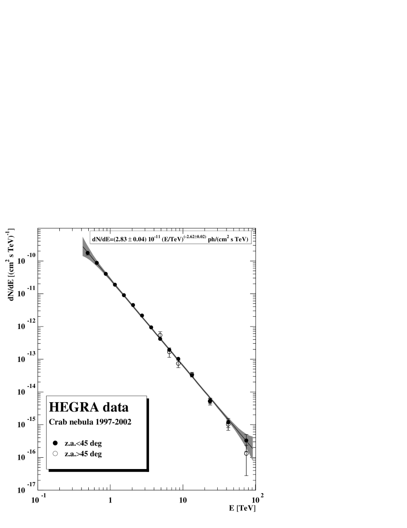
Figure 3: As a result of the spectral analysis in two different zenith angle intervals (6.2^∘-45^∘,45^∘-65^∘), the differential energy spectrum covers the range from 0.5 TeV up to 100 TeV. The significance of the data point centered on 86 TeV is 2.7 $\sigma$ after combining the events from all zenith angles. The grey shaded region indicates the range of systematic errors which are most prominent in the threshold region where the statistical errors are smaller than the systematic uncertainties.

The reconstructed differential energy spectra for two different ranges in zenith angle are shown in Fig. 3. Systematic uncertainties are estimated based upon possible variations in the threshold region unaccounted for in the simulations, uncertainties in the nonlinear response of the PMTs and read-out chain at high signal amplitudes. The range of systematic uncertainties is indicated by the grey shaded region in Fig. 3. In addition to the energy dependent uncertainties shown by the grey shaded region, the global energy scale is uncertain within 15 %.

The dominating uncertainties are visible in the threshold region above 500 GeV. The estimate of the systematic uncertainties is shown to be quite conservative judging from the smooth connection of the flux measured at small zenith angles with the flux measured at larger zenith angles at $\approx 6$ TeV. The flux measured at the threshold for the data set with zenith angles larger than $45^{\circ}$ is in very good agreement with the measurement from smaller zenith angles.

Additionally, the good agreement of the two different energy spectra at very high energies shows that the systematic effect of the nonlinear response at high signal amplitudes is probably smaller than estimated. The nonlinear response affects mainly the small zenith angle observations where for a given energy of the shower the average image amplitude is much higher (by a factor of $4\ldots 6$) than for larger zenith angles. The effect of the saturation/nonlinearity is expected to be negligible at larger zenith angles. The good agreement shows that the correction applied to the high signal amplitudes is accurate.

For the purpose of combining data taken at different zenith angles, the same approach as described in Aharonian et al. (2000b) is followed. The combined energy spectrum (Table 3) is well approximated by a pure power law of the form $d\Phi/dE=\Phi_{0}\cdot(E/\mathrm{TeV})^{\Gamma}$ with $\Phi_{0}=(2.83\pm 0.04_{\mathrm{stat}}\pm 0.6_{\mathrm{sys}})$ $\cdot 10^{-11}$ ph cm^-2 s^-1 TeV^-1and $\Gamma=-2.62\pm 0.02_{\mathrm{stat}}\pm 0.05_{\mathrm{sys}}$. The $\chi^{2}_{red}(d.o.f.)=1.3(13)$ indicates that deviations from a power law do not appear to be very significant. The systematic errors quoted on the parameters are the result of varying the data points within the systematic errors (the grey shaded band in Fig. 3) and for the normalization $\Phi_{0}$ the uncertainty of the energy scale is included.

Even though a power law fit to the data is a good approximation without statistically significant deviations, a systematic deviation from a power law in the form of a steepening can be seen upon closer inspection (see also Fig. 11) and will be discussed in Section 5.3.

4.2 Source position and morphology

In a previous HEGRA paper (Aharonian et al., 2000a), the emission size region of the Crab nebula for energies up to 5 TeV has been constrained with a smaller data-set (about one third of the data used here) to be less than 1.7 arc min .

Here, results from a similar analysis technique are presented. The most noticeable difference with respect to the previously published results is that the upper limits are calculated within 7 independent energy bins covering the energy range from 1 to 80 TeV. In principle, an ionic component in the wind could be a rather narrow feature in the energy spectrum and therefore might have gone unnoticed in an analysis using the integral distribution of all gamma-ray events.

Taking all data, the center of the emission region is determined to be r.a.=$5^{h}34^{m}(31.1\pm 0.2_{\mathrm{stat}}\pm 1.8_{\mathrm{sys}})^{s}$, $\delta=22^{\circ}0^{\prime}(52\pm 3_{\mathrm{stat}}\pm 25_{\mathrm{sys}})^{\prime\prime}$ (J2000) which is shifted by $(12.4\pm 3.1_{\mathrm{stat}}\pm 25_{\mathrm{sys}})$^′′ angular distance to the west of the nominal position of the pulsar (J2000.0) r.a.=$5^{h}34^{m}31.97^{s}$, $\delta=22^{\circ}0^{\prime}52.1^{\prime\prime}$ (Han & Tian, 1999). This shift is consistent with the expectation based upon the centroid position of the X-ray emitting nebula. The centroid position of the X-ray emitting nebula derived from public Chandra data of the Crab excluding the pulsar emission is shifted by 9^′′ to the west. In declination the position of the TeV emission region is consistent with the position of the pulsar: ($1.9\pm 3.0_{\mathrm{stat}}\pm 25_{\mathrm{sys}}$)^′′ angular distance. The centroid position of the X-ray emitting nebula as measured with the Chandra X-ray telescope is shifted to the north by 13^′′.

Checks on the data split into the yearly observation campaigns confirm the offset to be present throughout the observation time. The statistical uncertainty on the position is smaller than the observed shift in right ascension. However, given the systematic uncertainty of 25^′′ derived from the pointing calibration, it is not possible to identify the position of the emission region with the pulsar or with structures in the nebula. The shift remains constant for different energy bins as shown in Fig. 4.

The limits on the source extension $\sigma_{src}$ (with a confidence level of 99.865 %) are shown in Fig. 5. Clearly, a source size exceeding 2^′ can be excluded at energies below 10 TeV. At higher energies, the limit given here constrains the size to be less than 3^′. The expected source size in the leptonic model would be close to 20^′′ whereas for an ionic component the size of the emission region would exceed 3^′. Given the upper limits here, a narrow (in energy) emission component as predicted by Amato, Guetta, & Blasi (2003); Bednarek & Bartosik (2003) which could lead to an increase of the source size for energies where this emission component dominates, is not found. This is consistent with the upper limit derived on the fraction of the spin-down luminosity present in kinetic energy of ions in the wind (see Section 5).

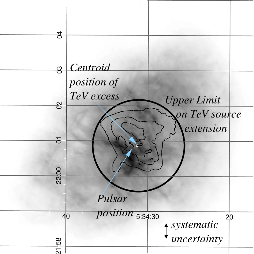
Figure 6: Shown in greyscale is the radio map of the Crab nebula combined with X-ray contours. The solid line circle indicates the upper limit on the TeV source size and as a white square the position of the TeV centroid (the sidelength indicate the 3^′′ statistical error).

In Fig. 6 the upper limit on the source extension between 3 and 5.6 TeV is compared with the radio (greyscale) and X-ray map (contours) taken from the Chandra Supernova Remnant Catalog. The solid circle indicates the upper limit on the TeV source size. The small white square depicts the position of the TeV emission centroid where the sidelength of the square is the statistical uncertainty on the position.

4.3 Phase resolved analysis

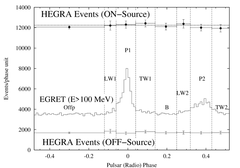
Figure 7: The phasogram of the Crab emission at two different energies: EGRET measurements show above 100 MeV a bimodal distribution. The different characteristic pulse intervals are marked (see text for further details). For the entire HEGRA data-set the ON-source and OFF-source distribution in the same phase bins is shown without evidence for a signal.

The phasogram obtained by folding the events registered from the direction of the Crab pulsar and a background region are shown in Fig. 7 together with the phasogram obtained with EGRET at lower energies (Fierro, Michelson, Nolan, & Thompson, 1998). Additionally, the search for pulsed emission is carried out on short data-sets covering a month each. This is a test to check whether unnoticed long term instability effects of the GPS timing information might have smeared a signal after combining data taken over long periods of time. The distribution of probabilities derived from the various tests (Rayleigh and $Z_{2}^{2}$) is consistent with being uniform for ON and OFF source data. No episodic excess is observed.

In the absence of a pulsed signal, upper limits are calculated. The strong persistent signal of the Crab nebula is causing a substantial background to a possible pulsed signal and needs to be considered for the calculation of upper limits.

The method described in Aharonian et al. (1999a) is used to constrain a possible pulsed fraction of the unpulsed flux. Here, we use the main pulse (P1) region between the phase $-0.06$ and $0.04$ to derive upper limits at the confidence level of 99.865  % ($3~{}\sigma$).

The upper limits for 7 bins of energy are summarized in Table 4 and shown in Fig. 8 together with results from EGRET (Fierro, Michelson, Nolan, & Thompson, 1998) and ground-based gamma-ray detectors: CAT (Musquere et al., 1999), Whipple (Lessard et al., 2000), and CELESTE (de Naurois et al., 2002). The HEGRA upper limits are marginally dependent on the assumed energy spectrum because they are calculated differentially for narrow energy bins. In order to compare these values with other published (integral) upper limits, a differential power law type spectrum has been assumed. Notably, the HEGRA upper limits cover a wider energy range than the other results and reach the lowest value in this range. Furthermore, the upper limits are independent for each energy band whereas all other quoted upper limits are integral limits which are less sensitive to narrow features in the spectrum.

The model predictions for outer gap emission as calculated recently by Hirotani & Shibata (2001) are partially excluded by the upper limits presented here. However, the expected flux from the Crab pulsar is strongly depending upon the opacity of the acceleration site for very high energy photons. The opacity is governed by the ambient soft photon density and the strength of the magnetic field. The optimistic cases considered with the gap sufficiently far away from the pulsar and low ambient photon density are nominally excluded by the upper limits given here. As has been pointed out (Hirotani, private communication) further absorption of photons by single photon-pair production is expected and will reduce the expected flux considerably. The predictions of this model need to be revised and will not be constrained by this observation.

5 Model calculations for the emission from the nebula and Discussion

5.1 Broad band spectral energy distribution

For the purpose of calculating the inverse Compton scattered radiation, three basic photon fields need to be taken into account:

• Synchrotron emission: This radiation field dominates in density for all energies and is the most important seed photon field present.

• Far infrared excess: Observations at far-infrared wavelengths have shown the presence of possibly thermal emission which exceeds the extrapolation of the continuum emission from the radio band. This component is best described by a single temperature of 46 K (Strom & Greidanus, 1992). Unfortunately, the spatial structure of the dust emission remains unresolved which introduces uncertainties for the model calculations. We have assumed the dust to be distributed like the filaments with a scale-length of 1.3^′. Sophisticated analyses of data taken with the ISO satellite indicates that the dust emission can be resolved (Tuffs, private communication). The resulting size seems to be consistent with the value assumed here.

• Cosmic Microwave Background (CMB): Given the low energy of the CMB photons, scattering continues to take place in the Thomson regime even for electron energies exceeding 100 TeV (Aharonian & Atoyan, 1995).

The influence of stellar light has been found to be negligible (Atoyan & Aharonian, 1996). The optical line emission of the filaments is spatially too far separated from the inner region of the nebula where the very energetic electrons are injected and cooled. However, in the case of acceleration taking place at different places of the nebula, the line emission could be important.

Given the recent detection of a compact component emitting mm radiation (Bandiera, Neri, & Cesaroni, 2002) this radiation field is included as seed photons for the calculation of the inverse Compton scattering. A simple model calculation has been performed which follows the phenomenological approach suggested by Hillas et al. (1998).

In brief, the observation of the continuum emission from the nebula up to MeV energies is assumed to be synchrotron emission. By setting the magnetic field to a constant average value within the nebula, a prompt electron spectrum can be constructed that reproduces the observed spectral energy distribution. Based upon the measured size of the nebula at different wavelengths, the density of electrons and the produced synchrotron photons can be easily calculated in the approximation that the radial density profile follows a Gaussian distribution.

With this simple model, it is straight-forward to introduce additional electron components and seed photon fields to calculate the inverse Compton scattered emission of the nebula. The model is described in more detail by Horns & Aharonian (2004).

In order to extract the underlying electron spectrum, a broad band SED is required (see Fig. 9). For the purpose of compiling and selecting available measurements in the literature, mostly recent measurements have been chosen. The prime goal of the compilation is to cover all possible wavelengths from radio to gamma-ray. The radio data are taken from (Baars & Hartsuijker, 1972) and references therein, mm data from (Mezger et al., 1986; Bandiera, Neri, & Cesaroni, 2002) and references therein, and the infrared data obtained with IRAS in the far- to mid-infrared (Strom & Greidanus, 1992) and with ISO in the adjacent mid- to near-infrared band (Douvion, Lagage, Cesarsky, & Dwek, 2001).

Optical and near-UV data from the Crab nebula require some extra considerations. The reddening along the line-of-sight towards the Crab nebula is a matter of some debate. For the sake of homogeneity, data in the optical (Veron-Cetty & Woltjer, 1993) and near-UV and UV (Hennessy et al., 1992; Wu, 1981) have been corrected applying an average extinction curve for $R=3.1$ and $E(B-V)=0.51$ (Cardelli, Clayton, & Mathis, 1989).

The high energy measurements of the Crab nebula have been summarized recently in Kuiper et al. (2001) to the extent to include ROSAT HRI, BeppoSAX LECS, MECS, and PDS, COMPTEL, and EGRET measurements covering the range from soft X-rays up to gamma-ray emission. For the intermediate range of hard X-rays and soft gamma-rays, data from Earth occultation technique with the BATSE instrument have been included (Ling & Wheaton, 2003).

The observations of the Crab nebula at very high energies (VHE, $E>100$ GeV) have been carried out with a number of ground based detectors. Most successfully, Cherenkov detectors have established the Crab nebula as a standard candle in the VHE domain. A summary of the measurements is presented in Aharonian et al. (2000b). Recently, the MILAGRO group has published a flux estimate which is consistent with the measurement presented here (Atkins et al., 2003).

The results from different detectors reveal underlying systematic uncertainties in the absolute calibration of the instruments. To extend the energy range covered in this work (0.5-80 TeV), results from non-imaging Cherenkov detectors like CELESTE (open circle), STACEE (solid square), and GRAAL (open diamond) at lower energy thresholds have been included (de Naurois et al., 2002; Oser et al., 2001; Arqueros et al., 2002), converted into a differential flux assuming a power law for the differential energy spectrum with a photon index of $2.4$. For energies beyond 100 TeV, an upper limit on the integral flux from the CASA-MIA air shower array has been added (Borione et al., 1997) assuming a power law with a photon index of $3.2$ as predicted from the model calculations.

The resulting broad band SED is shown in Figure 9 including as solid lines the synchrotron and inverse Compton emission as calculated with the electron energy distribution assumed in this model. Also indicated as a dotted line in Fig. 9 is the thermal excess radiation which is assumed to follow a modified black body radiation distribution with a temperature of 46 K. Finally, the emission at mm-wavelengths is indicated by a thin broken line (see also Section 5.2). The thick broken line indicates the synchrotron emission excluding the thermal infrared and non-thermal mm-radiation. The inverse Compton emission shown in Fig. 9 includes the contribution from mm emitting electrons (see next section).

Besides the spectral energy distribution, an estimate of the volume of the emitting region is required to calculate the photon number density in the nebula to include as seed photons for inverse Compton scattering. The size of the nebula is monotonically decreasing with increasing photon energies which is predicted in the framework of the MHD flow models (Atoyan & Aharonian, 1996; Amato et al., 2000).

The result of the calculation for the inverse Compton emission are tabulated separately for the different contributions from the seed photon fields in Table 5. The table lists the differential flux in the commonly used units photons $\mathrm{TeV}^{-1}\mathrm{cm}^{-2}\mathrm{s}^{-1}$ which can be converted directly into energy flux by multiplying with the squared energy. For convenience, Table 6 gives the coefficients for a polynomial parameterization of the energy flux as a function of energy in a double logarithmic representation with a relative linear accuracy better than 4 %.

5.2 Impact of a compact emission region at mm-wavelengths

The recently found emission region at mm-wavelengths (Bandiera, Neri, & Cesaroni, 2002) is more compact than the radio and optical emission region. In the current calculation, this emission region is modeled by an additional synchrotron emission component with a Gaussian equivalent radial width of 36^′′ as derived from Fig. 5 of (Bandiera, Neri, & Cesaroni, 2002). The electrons radiating at mm-wavelengths produce also an additional inverse Compton component at GeV energies which partially reduces the discrepancy between the observed and predicted gamma-ray emission between 1 and 10 GeV. As a note, in order to match the EGRET flux, the mm-emission region would have to be roughly half ($\approx 16$^′′) of the size used for this calculation.

As pointed out in Bandiera, Neri, & Cesaroni (2002), a thermal origin is ruled out for several reasons which leaves the possibility of synchrotron emission. The origin of the mm emitting electrons is unclear. Contrary to the common picture of a relic electron population that was possibly emitted at an earlier stage of the nebula’s development (see also Section V of Kennel & Coroniti (1984b) for a discussion on the problems to produce such a radio component in the framework of the MHD flow model), the mm electrons are apparently confined to or possibly injected into a similar volume as the soft X-ray emitting electrons.

The extra component can be explained by a population of electrons with a minimum Lorentz factor of $\approx 10^{4}$ and a maximum Lorentz factor of $\approx 10^{6}$ with a power law index $p$ close to 2 ($dN/d\gamma=N_{0}\,\gamma^{-p}$). In order to inject such an electron distribution, a small scale shock is required at a distance of $\approx 10^{14}$ cm distance to the pulsar. The maximum Lorentz factor reachable in the downstream region scales with the curvature radius of the shock. The minimum Lorentz factor according to the Rankine-Hugoniot relations for a shock at $10^{14}$ cm is $\approx 10^{4}$ provided that the spectral index is $\approx 2$ for the particle distribution. In recent magneto-hydrodynamic calculations (Bogovalov & Khangoulian, 2002; Komissarov & Lyubarsky, 2003) the observed jet-torus morphology of the Crab nebula is reproduced by invoking a modulation of the flow speed with $\sin\theta^{2}$ ($\theta$ is the polar angle with respect to the rotation axis of the pulsar). This assumption is motivated by the solution for the wind flow in the case of an oblique rotator assuming a split monopole magnetic field configuration (Bogovalov, 1999). According to the calculation of Komissarov & Lyubarsky (2003), a multi layered shock forms. In the proximity of the polar region the shock would form close to the pulsar and could be responsible for the injection of mm-emitting electrons.

This shock region has remained undetected because of the angular proximity (10 mas) to the pulsar and the fact that the continuum emission is predominantly produced in the mm and sub-mm wavelength band. The inner shock is in principle visible with high resolution observations with interferometers at mm wavelengths.

Intriguingly, there is observational evidence for ongoing injection of electrons radiating at 5 GHz frequency which show moving wisp-like structures similar to the optical wisps (Bietenholz & Kronberg, 1992; Bietenholz, Frail, & Hester, 2001). The injection of radio- and mm-emitting electrons into the nebula could e.g. take place at additional shocks much closer to the pulsar than the previously assumed $14$^′′.

The additional compact mm component is of importance for the inverse Compton component: The electron population with $\gamma=10^{4}\ldots 10^{5}$ introduced here to explain the excess at mm-wavelengths produces via inverse Compton scattering gamma-rays between 1 and 10 GeV. The contribution is rather small (10 %) but could easily become comparable to the other components if the mm-emitting region is smaller than assumed here. In this case, the EGRET data points would be better described by the model. Moreover, the mm component contributes seed photons for inverse Compton scattering in the Thomson regime which contributes substantially at energies of a few TeV.

The combined inverse Compton spectrum is shown in Fig.10 decomposed according to the different seed photons (Sy, IR, mm, CMB) and the additional inverse Compton component from the mm-emitting electrons. Clearly, the synchrotron emission present in the nebula is the most important seed photon field present. At high energies ($E>10$ TeV) the mm-radiation is contributing significantly to the scattered radiation.

5.3 Comparison of the model with data

The agreement of the calculated inverse Compton spectrum with the data is excellent (see Fig. 10). The only free parameter of the model calculation is the magnetic field which in turn can be determined from the data by minimizing the $\chi^{2}$ of the data (see Section 5.4). The resulting value of $\chi^{2}$ is slightly lower than for the power-law fit: $\chi^{2}_{red}(d.o.f)=0.96(14)$ for the inverse Compton model as compared with $\chi^{2}_{red}(d.o.f.)=1.3(13)$. However, the small change in $\chi^{2}$ does not convey the full information. The slope of the spectrum is expected to change slightly with energy for the inverse Compton model. For the purpose of testing this gradual softening predicted in the model, the differential power-law was calculated from the data points by computing the slope between two data-points with index $i,j$ separated by 0.625 in decadic logarithm.

$$\Gamma(E) = \frac{\ln\Phi_{i}-\ln\Phi_{j}}{\ln E_{i}-\ln E_{j}}$$ (4)

$$E = \exp(0.5\cdot(\ln E_{i}+\ln E_{j}))$$ (5)

$$\sigma_{\Gamma} = \frac{\sqrt{(\sigma_{\Phi(i)}/\Phi_{i})^{2}+(\sigma_{\Phi(j)}/\Phi_{j})^{2}}}{\ln E_{i}-\ln E_{j}}$$ (6)

For the sake of simplicity, the error on $E_{i},E_{j}$ is ignored. The effect of including the statistical error on $E_{i},E_{j}$ is negligible. The interval of 0.625 in decadic logarithm gives sufficient leverage to calculate a reliable slope and at the same time it is small enough to resolve the features. The expected slope is calculated from the model for both cases including and excluding the mm seed photon field. The result is shown in Fig. 11. The straight broken line is the predicted slope as given by the parameterization of Hillas et al. (1998), the open symbols indicate the prediction from Aharonian (1998) which are consistent with the calculation described here. Note, the data points are independent. As is clearly seen, the expected and measured change in slope agree nicely. The systematic and energy dependent deviation from the constant photon index determined by the power law fit is evident. Ignoring the mm-component gives on average a slightly softer spectrum with the same softening with increasing energy. It is remarkable how little the slope is expected to change over exactly the energy range covered by the observations. Going to energies below 200 GeV, a strong flattening of the energy spectrum is to be expected. At the high energy end, beyond roughly 70 TeV the softening is expected to be stronger.

5.4 The average magnetic field

The average magnetic field is calculated by minimizing the $\chi^{2}$ of the model with respect to the data varying the magnetic field as a free parameter. For every value for the magnetic field, the break energies and normalization of the electron spectrum is chosen to reproduce the synchrotron spectrum.

The resulting $\chi^{2}$ as a function of magnetic field shows a minimum at $161.6~{}\mu$G with $\chi^{2}_{red}(d.o.f.)=0.96(14)$. The $1\sigma$ statistical uncertainty of $0.8~{}\mu$G is negligible. The systematic uncertainties of $15~{}$% on the absolute energy scale of the measurement translates into a systematic error on the average magnetic field of 18 $\mu$G.

5.5 Gamma-ray emission from ions in the wind

As has been pointed out independently by Amato, Guetta, & Blasi (2003) and Bednarek & Bartosik (2003) the presence of ions in the relativistic wind could be detected by the production of neutrinos and gammas in inelastic scattering processes with the matter in the nebula. Neutrinos and gammas would be produced as the decay products of charged and neutral pions. Both calculations show a similar signature for the ion induced gamma-ray flux which appears as a rather narrow feature in a $\nu f_{\nu}$ diagram. The presence of ions is required in acceleration models in which positrons in the downstream region are accelerated by cyclotron waves excited by ions (Arons, 1995).

Qualitatively, the ions in the pulsar wind fill the nebula without undergoing strong energy losses. For a typical bulk velocity of the wind of $\Gamma=10^{6}$, the dominant energy losses are adiabatic expansion of the nebula and escape of particles with typical time scales of the order of the age of the remnant. Therefore, the almost monoenergetic distribution of the ion energies as it is injected by the wind is not widened significantly in energy.

From the model calculations described above, the TeV data are well explained by inverse Compton scattering of electrons present in the nebula. The shape and the absolute flux measured is consistent with the prediction of this model. However, an admixture of gamma-ray emission processes of electrons and ions could be possible. In an attempt to estimate how much of the spin down power of the pulsar could be present in the form of ions, a model calculation for the gamma-ray emission from ions in the wind is performed. Here, 99 % c.l. upper limits are calculated on the fraction $\zeta$ of the spin down luminosity present in ions ($L_{ion}=\zeta\dot{E}_{pulsar}$) by adding the additional component to the inverse Component component and comparing this prediction with the data. The $\chi^{2}$ of the combined prediction is calculated for different values of $\zeta$ until the $\chi^{2}$ increases by $\Delta\chi^{2}=29.15$ for a 99 % confidence level. This calculation is repeated for various values of $\Gamma$.

The calculation of the gamma-ray flux from the ions depends upon a few simplifications. It is assumed that the ions are predominantly protons with a narrow energy distribution with $E_{p}\approx\Gamma m_{p}c^{2}$. For the injection rate of protons $\dot{N}_{p}=\zeta\dot{E}_{pulsar}/E_{p}$ with $\dot{E}_{pulsar}=5\cdot 10^{38}$ erg s^-1 is assumed. The injection rate of $\pi^{0}$ is depending on the conversion efficiency: $\dot{N}_{\pi}=f_{\pi}\dot{N}_{p}$. The conversion efficiency $f_{\pi}$ of the protons to $\pi^{0}$ is given by the ratio of energy loss time scales for pp-scattering and escape/adiabatic losses. Assuming an average number density of the gas in the nebula of 5 cm^-3, the conversion efficiency is $5.4\times 10^{-5}$.

The upper limits for $\zeta$ as a function of the bulk Lorentz factor are given in Fig. 12. Clearly, for bulk Lorentz factors between $10^{4}$ to $10^{6}$, only a small fraction of the energy carried by the wind could be present in the form of ions ($<20$ %). For Lorentz factors beyond $10^{6}$ or smaller $10^{4}$ a substantial part of the power could be injected in the form of ions.

However, the assumption of a narrow energy distribution might not be true. In the case of a variation of the wind speed as discussed above in the context of a split magnetic monopole model, the injected ions could have a wider distribution in energy which subsequently makes an identification of this feature in the measured gamma-ray spectrum more complicated and upper limits calculated less restrictive.

5.6 Additional Components

The presence of additional electron populations in the nebula with $\gamma>10^{5}$ can be constrained by the gamma-ray data presented here. Obviously, the observed synchrotron emission already excludes the presence of components not accounted in the model calculations presented in Section 5. However, the frequency interval between hard UV and soft X-ray emission is not covered by observations and large systematic uncertainties on the strong absorption present would in principle not exclude the presence of an additional component that is sufficiently narrow in energy. Specifically, electrons following a relativistic Maxwellian type distribution may form in the framework of specific acceleration models (Hoshino et al., 1992). For the magnetic field of 161 $\mu$G, UV-emitting electrons would have $\gamma\approx 10^{7}$. Given the age of the nebula of 954 years, the synchrotron-cooled spectrum is close to a power-law with $dN/d\gamma\propto\gamma^{-2}$ reaching to $\gamma_{min}=10^{6}$. The resulting synchrotron emission is not in conflict with the available data unless the power in the extra Maxwellian type injection spectrum becomes a sizable fraction ($L_{Maxw.}/L_{tot}>0.3$) of the total power of the electrons responsible for the broad-band SED. However, after calculating the inverse Compton emission of this extra component and comparing it with the gamma-ray data, an upper limit at 99 % c.l. can be set $L_{Maxw.}/L_{tot}<0.04$ ruling out the existence of unnoticed (unobserved) electron populations with $\gamma=10^{6}\ldots 10^{7}$ in the nebula The possible existence of an additional synchrotron emitting component possibly associated with a spectral hardening in the MeV energy range as observed consistently by the COMPTEL instrument (Much et al., 1995), BATSE (Ling & Wheaton, 2003), and INTEGRAL (Roques et al., 2003) and has been discussed e.g. in DeJager (2000). The contribution of such an additional component to the observed TeV flux is probably small and is relevant only at energies exceeding a few 100 TeV.

6 Summary and Conclusions

The HEGRA stereoscopic system of air Cherenkov telescopes performed extensive observation of the Crab supernova remnant. The energy spectrum has been determined over more than 2 decades in energy and 5 decades in flux. The main points of the data analyses are to constrain the acceleration of electron/positron pair plasma in the vicinity of the termination shock of the pulsar wind in the surrounding medium. The high energy data presented here give a unique view on the extreme accelerator which resides in the Crab nebula.

The energy spectrum of the unpulsed component is very likely produced by the same electrons that produce the broad-band emission spectrum extending from soft to hard X-rays and finally reach the soft gamma-rays (with a cut-off at a few MeV). The electrons up-scatter mainly photons of the synchrotron nebula, the soft thermal photons seen as the far infrared excess, the universal cosmic microwave background (CMB), and possibly mm-radiation emitted in a rather compact region.

The comparison of the flux level at TeV energies combined with the synchrotron flux in a simple spherical model, constrains directly the magnetic field in the emission region of the nebula to be at the level of 160 $\mu$G. The agreement of the measured broad band energy spectrum ranging from soft X-rays up to 100 TeV with the prediction based upon a simple model of an electron population being injected at the standing reverse shock strengthens the claim that electrons with energies exceeding $10^{15}$ eV are continuously accelerated. Limited by the photon statistics detected at high energies ($>10$ TeV), expected variations in the acceleration/cooling rate on time scales of months for these electrons can not be established with the current instrumentation.

The data show evidence for the predicted gradual softening of the energy spectrum. Below roughly 200 GeV the spectrum is expected to harden quickly. Future detectors with a sufficiently low energy threshold will be able to see this feature. However, the expected softening occurs rapidly at energies beyond 70 TeV. Here, low elevation observations with the Cherenkov telescopes from the southern hemisphere will be very helpful.

Given the good agreement of the predicted inverse Compton spectrum with the measurement, the presence of ions in the wind is either negligible or radiative losses are exceedingly small. Independent of the spectrum, the morphology of the emission region could reveal signatures of the presence of ions in the wind and the nebula. Experimental upper limits given here constrain the size of the emission region at the considered energies to be less than 2^′ and less than 3^′ above 10 TeV. This excludes for example a strong contribution from the outer shock of the (undetected) expanding super nova remnant and constrains the transport of ions in the wind.

Finally, pulsed emission from inside the pulsar’s magnetosphere at high energies is expected in outer gap models. A dedicated search for narrow features as predicted in this type of model has been performed and in the absence of a signal, upper limits have been calculated. The upper limits reach well below the more optimistic predictions of Hirotani & Shibata (2001) but more recent calculations indicate that the pair opacity in the emission region is possibly larger than originally anticipated. In a different scenario, pulsed emission is expected to arise as a consequence of inverse Compton scattering of pulsed soft photons by the un-shocked wind (Bogovalov & Aharonian, 2000). The upper limits derived here are useful in constraining combinations of the bulk Lorentz factor and the distance of wind injection to the pulsar. For a range of bulk Lorentz factors from $10^{5}-10^{7}$ the distance of the wind is constrained to be accelerated more than 50 light radii away from the pulsar.

7 Outlook

Future observations of the nebula with low energy threshold instruments (MAGIC, GLAST) and large collection area observations at small elevations from the southern hemisphere (CANGAROO III, H.E.S.S.) should extend the accessible energy range below 100 GeV (MAGIC) and beyond 100 TeV (CANGAROO III, H.E.S.S.) where the spectral shape is expected to deviate strongly from a power-law with $\Gamma=-2.6$. With low energy threshold Cherenkov telescopes like MAGIC the detection of pulsed emission from the pulsar becomes feasible. Combining information about possible variability of the nebula’s emission at different wavelengths (specifically hard X-rays and say 20-100 TeV emission) would ultimately prove the common (electronic) origin of the observed emission. Fortunately, the Crab will be frequently observed as a calibration source by all Cherenkov telescopes and by INTEGRAL and other future hard X-ray missions so that even without dedicated observations, substantial observation time will be accumulated. A dedicated mm-observation with sub-arcsecond resolution of the region of the nebula within the X-ray torus would be of great interest in order to confirm the predicted existence of multi-layered shocks which could be responsible for the mm-emission detected with the moderate ($>$ 10^′′) resolution observations currently available. If the injection of mm-emitting electrons in a compact region is confirmed, inverse Compton scattered emission produced by the same low energy electrons could in principle explain the discrepancy of the model with the energy spectrum observed by the EGRET spark-chamber onboard the CGRO satellite. Again, future observations with the GLAST satellite with improved statistics will be of great interest to study the actual shape of the energy spectrum above a few GeV.

Figure 1: As a check for unnoticed temporal changes in the instrumental response, the integrated fluxes for the five observing years are compared with each other. The respective values are normalized to the integral flux derived from the power-law fit to the entire data-set. As is clearly seen from the relative deviations of $\Phi(E>1~{}\mathrm{TeV})$ systematic effects are smaller than 10 % indicated by the dashed lines which translates into a relative uncertainty of the absolute energy calibration of better than 6 % (assuming a power law type spectrum with an index of -2.62). The integrated fluxes above 5.62 TeV show larger fluctuations which are still consistent with a constant flux.

Figure 2: As a function of reconstructed energy, the size of the point spread function observed from the Crab nebula does not differ from the predicted values from simulation (dashed and solid lines indicate average and 1$~{}\sigma$ uncertainty.)

Figure 4: As a function of reconstructed energy, the position of the emission region does not show significant variation. The open symbols indicate the deviation of the reconstructed declination to the declination of the pulsar ($\Delta\delta$), filled symbols indicate the deviation of the right ascension ($\Delta$ r.a.).

Figure 5: Based upon the predicted point-spread function from simulation 3$\sigma$ upper limits for a Gaussian type source size have been calculated. These are independent (differential) upper limits improving sensitivity for a particular narrow (in energy) feature expected from an ionic component in the wind.

Figure 8: Result of a search for pulsed gamma-ray emission with HEGRA (upper limits indicated by filled squares). The integral upper limits quoted for the CAT, CELESTE, and Whipple group have been converted by assuming a differential spectral index of -2.4 at energies below 1 TeV and -2,6 above 1 TeV. For comparison, the energy spectrum for the main pulse as detected by the EGRET spark chamer is shown by filled triangles. The existence of a cut-off is expected in most theoretical models which propose the origin of the Gamma-rays to be close to the polar cap or the magnetosphere (outer gap). The upper limits shown are consistent with the picture of a cut-off at a few ten GeV. The solid line is fit of a power-law function with photon index $\Gamma=-2.08$ and an exponential cut-off at 25 GeV to the EGRET data and the CELESTE upper-limit as suggested in Durand (2003). The dotted line are the synchrotron and inverse Compton emission of the nebula as given by the model prediction explained in the text.

Figure 9: For a wide range of energies, recent measurements have been compiled from the literature (see the text for further details and references). The curves are calculations described in Section 5.

Figure 10: The inverse Compton spectrum is decomposed into different components as defined by the target seed photons. The synchrotron radiation is dominating at all energies. However, the mm-excess is of equal importance above 30 TeV. Eventually, beyond 100 TeV, the microwave background is contributing significantly to the overall spectrum. Note, the contribution of the mm-radiation is dominating over the dust component at all energies. Also shown is the inverse Compton component from the electrons emitting the synchrotron mm-radiation. The symbols used are the same as for Fig. 9

Figure 11: The predicted photon index (line) changes only very little in the energy range considered and is consistent with the measured values (filled symbols).

Figure 12: For a variety of bulk Lorentz speeds of the wind, the fraction of the total spin down power which is injected in the form of ions is constrained to be less than 20 %. For Lorentz factors beyond $10^{6}$ and below $10^{4}$ a substantial fraction of the power could be present in the form of ions.

Table 1: Observational times

Season	$[6.5^{\circ},30^{\circ}[$	$[30^{\circ},45^{\circ}[$	$[45^{\circ},65^{\circ}]$	$\sum$	$\sum$
year	$[$ksec$]$	$[$ksec$]$	$[$ksec$]$	$[$ksec$]$	$[$hrs$]$
1997/98	165.68	125.47	75.94	367.08	101.97
1998/99	217.89	91.54	177.23	486.66	135.18
1999/00	89.35	28.67	0.81	118.83	33.00
2000/01	113.21	67.46	6.40	187.08	51.97
2001/02	95.94	100.30	29.61	225.84	62.73
Total	682.07	413.43	289.99	1385.49	384.86

Note. — Data after selection for good weather

Table 2: Image and event selection for different analyses

Selection	Spectrum	Morphology	Pulsation
Angular distance to source	$\vartheta<0.225^{\circ}$	no cut	$\vartheta<0.118^{\circ}$
Image shape	$\tilde{w}<1.1$	$\tilde{w}<1.1$	$\tilde{w}<1.1$
Image amplitude	$size>40$ p.e.	$size>40$ p.e.	$size>40$ p.e.
Image centroid position	$distance<1.7^{\circ}$	no cut	no cut
Estimated error on rec.	no cut	$\sigma_{sx}<0.1^{\circ}(0.06^{\circ})$	no cut
event direction
Core position	$r<200(400)\tablenotemark{b}$ m	no cut	no cut
Stereo Angle	$min(stereo)>20^{\circ}(10^{\circ})\tablenotemark{c}$	no cut	no cut
Number of images	$n_{image}\geq 3$	$n_{image}\geq 2$	$n_{image}\geq 2$
Zenith angle	$z.a.<65^{\circ}$	$z.a.<65^{\circ}$	$z.a.<65^{\circ}$

Table 3: Differential energy spectrum

$\langle E\rangle$	$E_{\mathrm{low}}-E_{\mathrm{high}}$	$d\Phi/dE\pm\sigma_{stat}$	$N_{on}$	$N_{off}$	$S$
$[\mathrm{TeV}]$	$[\mathrm{TeV}]$	$[(\mathrm{cm}^{2}\,\mathrm{s}\,\mathrm{TeV})^{-1}]$			$[\sigma]$
0.365	0.316-0.422	$(1.97\pm 1.17)\cdot 10^{-10}$	105	333	3.9
0.487	0.422-0.562	$(1.76\pm 0.24)\cdot 10^{-10}$	369	705	14.1
0.649	0.562-0.750	$(8.78\pm 0.53)\cdot 10^{-11}$	1012	1356	29.8
0.866	0.750-1.000	$(4.02\pm 0.13)\cdot 10^{-11}$	2119	2108	50.0
1.155	1.000-1.334	$(1.87\pm 0.09)\cdot 10^{-11}$	2829	2772	58.2
1.540	1.334-1.778	$(9.05\pm 0.26)\cdot 10^{-12}$	2458	2220	56.1
2.054	1.778-2.371	$(4.51\pm 0.12)\cdot 10^{-12}$	2017	1600	48.9
2.738	2.371-3.162	$(2.16\pm 0.07)\cdot 10^{-12}$	1510	1114	47.3
3.652	3.162-4.217	$(9.33\pm 0.36)\cdot 10^{-13}$	950	645	38.6
4.870	4.217-5.623	$(4.18\pm 0.20)\cdot 10^{-13}$	579	330	31.7
6.494	5.623-7.499	$(1.93\pm 0.12)\cdot 10^{-13}$	345	187	23.3
8.660	7.499-10.000	$(1.02\pm 0.07)\cdot 10^{-13}$	238	111	21.4
13.335	10.000-17.783	$(3.28\pm 0.31)\cdot 10^{-14}$	414	420	19.7
23.714	17.783-31.622	$(5.28\pm 0.70)\cdot 10^{-15}$	150	242	10.2
42.170	31.622-56.234	$(1.10\pm 0.25)\cdot 10^{-16}$	69	141	5.7
74.989	56.234-100.000	$(2.05\pm 1.01)\cdot 10^{-16}$	36	104	2.7

Table 4: Differential upper limits on pulsed emission

$\langle E\rangle$	$E_{low}-E_{high}$	fractional limit	flux limit
$[\mathrm{TeV}]$	$[\mathrm{TeV}]$	$[\%]$	$[10^{-14}$ ph (cm2 s TeV)${}^{-1}]$
0.548	0.32 - 1.00	3.3	392.5
1.414	1.00 - 2.00	2.4	29.6
2.828	2.00 - 4.00	2.8	6.03
5.657	4.00 - 8.00	4.3	1.32
11.314	8.00 - 16.00	7.4	0.41
22.627	16.00 - 32.00	7.1	0.05
56.569	32.00 - 100.0	43.4	0.02

Table 5: Predicted inverse Compton differential energy spectrum for different seed photons. The numbers (1-5) refer to the component with the respective label in Fig. 10

Energy	Total	1	2	3	4	5
$\log_{10}(\mathrm{E}/\mathrm{TeV})$	$\log_{10}(d\Phi/dE\cdot(\mathrm{cm}^{2}~{}\mathrm{s}~{}\mathrm{TeV}))$
-2.3835	-5.5682	-5.9685	-6.4142	-6.5613	-6.5423	-6.1671
-2.2168	-5.8493	-6.2340	-6.6881	-6.8169	-6.8950	-6.4603
-2.0501	-6.1358	-6.5045	-6.9685	-7.0784	-7.2499	-6.7664
-1.8835	-6.4293	-6.7811	-7.2561	-7.3481	-7.6054	-7.0891
-1.7168	-6.7305	-7.0644	-7.5515	-7.6295	-7.9614	-7.4289
-1.5501	-7.0412	-7.3557	-7.8558	-7.9268	-8.3177	-7.7880
-1.3835	-7.3618	-7.6561	-8.1704	-8.2436	-8.6747	-8.1660
-1.2168	-7.6932	-7.9668	-8.4962	-8.5827	-9.0324	-8.5616
-1.0501	-8.0372	-8.2903	-8.8345	-8.9416	-9.3908	-8.9833
-0.8835	-8.3966	-8.6298	-9.1860	-9.3135	-9.7503	-9.4553
-0.7168	-8.7994	-8.9893	-9.5500	-9.6927	-10.1109
-0.5501	-9.1819	-9.3752	-9.9242	-10.0780	-10.4731
-0.3835	-9.5879	-9.7950	-10.3056	-10.4700	-10.8368
-0.2168	-10.0108	-10.2403	-10.6928	-10.8694	-11.2027
-0.0501	-10.4374	-10.6914	-11.0862	-11.2773	-11.5710
0.1165	-10.8674	-11.1465	-11.4859	-11.6941	-11.9421
0.2832	-11.3010	-11.6052	-11.8925	-12.1209	-12.3166
0.4499	-11.7378	-12.0673	-12.3060	-12.5583	-12.6950
0.6165	-12.1785	-12.5325	-12.7267	-13.0072	-13.0782
0.7832	-12.6235	-13.0008	-13.1547	-13.4685	-13.4669
0.9499	-13.0730	-13.4722	-13.5905	-13.9431	-13.8621
1.1165	-13.5277	-13.9470	-14.0343	-14.4318	-14.2652
1.2832	-13.9885	-14.4258	-14.4868	-14.9353	-14.6784
1.4499	-14.4571	-14.9100	-14.9494	-15.4541	-15.1047
1.6165	-14.9366	-15.4021	-15.4246	-15.9887	-15.5496
1.7832	-15.4319	-15.9060	-15.9118	-16.5408	-16.0182
1.9499	-15.9477	-16.4287	-16.4345	-17.1204	-16.5060
2.1165	-16.4827	-16.9703	-16.9751	-17.7492	-17.0073
2.2832	-17.0254	-17.5166	-17.5249	-18.3934	-17.5230

Table 6: Polynomial coefficients for a fit to the total inverse Compton energy flux (corresponds to the second column in Table 5) of the form $\log_{10}\{\nu f_{\nu}/(\mathrm{erg}\,(\mathrm{cm}^{2}\,\mathrm{s})^{-1})\}=\sum_{i=0}^{5}p_{i}\log_{10}^{i}(E/\mathrm{TeV})$.

$p_{0}$	$p_{1}$	$p_{2}$	$p_{3}$	$p_{4}$	$p_{5}$
-10.3531	-0.578559	-0.119778	0.542375$\cdot 10^{-1}$	-0.766819$\cdot 10^{-2}$	-0.660223$\cdot 10^{-2}$

References

- Aharonian et al. (1993) Aharonian, F.A. et al. 1993, Towards a Major Atmospheric Cherenkov Detector, ed. R.C. Lamb (Calgary) 81
- Aharonian & Atoyan (1995) Aharonian, F. A. & Atoyan, A. M. 1995, Astroparticle Physics, 3, 275
- Aharonian (1998) Aharonian, F.A. in Frontiers Science Series 24, Neutron Stars and Pulsars, ed. N. Shibazaki, N. Kawai, S. Shibata, and T. Kifune (Tokyo:Universal Academy Press), 439
- Aharonian et al. (1999a) Aharonian, F., et al. 1999a, A&A346, 913-44
- Aharonian et al. (1999b) Aharonian, F. A., et al. 1999b, A&A, 349, 11
- Aharonian et al. (2000a) Aharonian, F. A., et al. 2000a, A&A, 361, 1073
- Aharonian et al. (2000b) Aharonian, F. A., et al. 2000b, ApJ, 539, 317
- Aharonian et al. (2000c) Aharonian, F., et al. 2000c, ApJ, 543, L39
- Aharonian (2000) Aharonian, F. A. 2000, New Astronomy, 5, 377
- Aharonian et al. (2001a) Aharonian, F., et al. 2001a, A&A, 370, 112
- Aharonian et al. (2001b) Aharonian, F. A., et al. 2001b, A&A, 375, 1008
- Aharonian et al. (2002a) Aharonian, F., et al. 2002a, A&A, 393, L37
- Aharonian et al. (2002b) Aharonian, F., et al. 2002b, A&A, 393, 89
- Aharonian et al. (2002c) Aharonian, F. A., et al. 2002c, A&A, 395, 803
- Aharonian et al. (2003a) Aharonian, F., et al. 2003a, A&A, 403, 523
- Aharonian et al. (2003b) Aharonian, F., et al. 2003b, A&A, 406, L9
- Amato, Guetta, & Blasi (2003) Amato, E., Guetta, D., & Blasi, P. 2003, A&A, 402, 827
- Amato et al. (2000) Amato, E., Salvati, M., Bandiera, R., Pacini, F., & Woltjer, L. 2000, A&A, 359, 1107
- Arons (1995) Arons, J. 1995, in ASP Conf. Ser. 72, Millisecond Pulsars: A Decade of Surprise, ed. A.S. Fruchter, M. Tavani, D.C. Backer (San Francisco:ASP), 257
- Arqueros et al. (2002) Arqueros, F. et al. 2002, Astroparticle Physics, 17, 293
- Atkins et al. (2003) Atkins, R., et al. 2003, ApJ, 595, 803
- Atoyan & Aharonian (1996) Atoyan, A. M. & Aharonian, F. A. 1996, MNRAS, 278, 525
- Baars & Hartsuijker (1972) Baars, J. W. M. & Hartsuijker, A. P. 1972, A&A, 17, 172
- Bandiera, Neri, & Cesaroni (2002) Bandiera, R., Neri, R., & Cesaroni, R. 2002, A&A, 386, 1044
- Bednarek & Bartosik (2003) Bednarek, W. & Bartosik, M. 2003, A&A, 405, 689
- Bennett et al. (1977) Bennett, K., et al. 1977, A&A, 61, 279
- Bietenholz, Frail, & Hester (2001) Bietenholz, M. F., Frail, D. A., & Hester, J. J. 2001, ApJ, 560, 254
- Bietenholz & Kronberg (1992) Bietenholz, M. F. & Kronberg, P. P. 1992, ApJ, 393, 206
- Blackman & Perna (2004) Blackman, E. G. & Perna, R. 2004, ApJ, 601, L71
- Bogovalov (1999) Bogovalov, S. V. 1999, A&A, 349, 1017
- Bogovalov & Aharonian (2000) Bogovalov, S. V. & Aharonian, F. A. 2000, MNRAS, 313, 504
- Bogovalov & Khangoulian (2002) Bogovalov, S. V. & Khangoulian, D. V. 2002, MNRAS, 336, L53
- Borione et al. (1997) Borione, A. et al. 1997, ApJ, 481, 313
- Buccheri et al. (1983) Buccheri, R., Bennett, K., Bignami, G.F. et al. 1983, A&A, 128, 245
- Bulian et al. (1998) Bulian, N., Daum, A., Hermann, G. et al. 1998, Astroparticle Physics 8, 223
- Cardelli, Clayton, & Mathis (1989) Cardelli, J. A., Clayton, G. C., & Mathis, J. S. 1989, ApJ, 345, 245
- Cheng, Ho, & Ruderman (1986) Cheng, K. S., Ho, C., & Ruderman, M. 1986, ApJ, 300, 500
- Coroniti (1990) Coroniti, F. V. 1990, ApJ, 349, 538
- Daum et al. (1997a) Daum, A., Hermann, G., Heß, M. et al. 1997, Astroparticle Physics 8, 1
- Daum et al. (1997b) Daum, A. et al. 1997, in Proc. of 25th ICRC, Vol. 5, ed MS Potgieter, BC Raubenheimer, and DJ van der Walt (Durban:Potschefstroomse Universiteit), 121
- DeJager et al. (1989) DeJager, O.C., Swanepoel, J.W.H., and Raubenheimer, B.C. 1989, A&A, 221, 180
- DeJager (2000) DeJager, O.C. 2000, High Energy Gamma-Ray Astronomy, AIP Vol 558, ed. F.A. Aharonian and H.J. Völk (Melville:AIP), 154
- de Naurois et al. (2002) de Naurois, M. et al. 2002, ApJ, 566, 343
- Dombrovsky (1954) Dombrovsky, V.A., 1954, Doklady Akad. Nauk SSSR, 94, 1021
- Douvion, Lagage, Cesarsky, & Dwek (2001) Douvion, T., Lagage, P. O., Cesarsky, C. J., & Dwek, E. 2001, A&A, 373, 28
- Durand (2003) Durand, E. 2003, Thèse de doctorat, Université Sciences et technologies, Bordeaux I
- Fierro, Michelson, Nolan, & Thompson (1998) Fierro, J. M., Michelson, P. F., Nolan, P. L., & Thompson, D. J. 1998, ApJ, 494, 734
- Franzen et al. (2003) Franzen, A., Gillessen, S., Hermann, G., and Hinton, J. 2003, in Procs. of 28th ICRC, Vol. 5, ed. T. Kajita, Y. Asaka, A. Kawachi, Y. Matsubara, and M. Sasaki (Tokyo:Universal Academy Press), 2987
- Gallant & Arons (1994) Gallant, Y. A. & Arons, J. 1994, ApJ, 435, 230
- Han & Tian (1999) Han, J. L. & Tian, W. W. 1999, A&AS, 136, 571
- Harding, Tademaru, & Esposito (1978) Harding, A. K., Tademaru, E., & Esposito, L. W. 1978, ApJ, 225, 226
- Hemberger (1998) Hemberger, M., PhD thesis, University of Heidelberg 1998
- Hennessy et al. (1992) Hennessy, G. S. et al. 1992, ApJ, 395, L13
- Hermann (1995) Hermann, G., 1995, Towards a Major Atmospheric Cherenkov detector IV, ed. M. Cresti (Padova:INFN), 396
- Hester et al. (1995) Hester, J. J., et al. 1995, ApJ, 448, 240
- Hester et al. (2002) Hester, J. J., et al. 2002, ApJ, 577, L49
- Hillas et al. (1998) Hillas, A. M. et al. 1998, ApJ, 503, 744
- Hirotani & Shibata (2001) Hirotani, K. & Shibata, S. 2001, ApJ, 558, 216
- Hofmann et al. (1999) Hofmann, W., Jung, I., Konopelko, A. et al. 1999, Astroparticle Physics, 12, 135
- Hofmann et al. (2000) Hofmann, W., Lampeitl, H., Konopelko, A., and Krawczynski, H. 2000, Astroparticle Physics 12, 207
- Hofmann (2003) Hofmann, W. 2003 Astroparticle Physics 20, 1
- Horns et al. (2003) Horns, D. et al. 2003, in Procs. of 28th ICRC, Vol. 5, ed. T. Kajita, Y. Asaka, A. Kawachi, Y. Matsubara, and M. Sasaki (Tokyo:Universal Academy Press), 2373
- Horns & Aharonian (2004) Horns, D. & Aharonian, F.A. 2004, ESA Special Publication SP-552 Proceedings of the 5th INTEGRAL Workshop in press
- Hoshino et al. (1992) Hoshino, M., Arons, J., Gallant, Y., and B. Langdon 1992 ApJ390, 454
- James (1998) James, F. 1998, CERN Program Library Long Writeup D506, CERN Geneva, Switzerland
- Kennel & Coroniti (1984a) Kennel, C. F. & Coroniti, F. V. 1984a, ApJ, 283, 694
- Kennel & Coroniti (1984b) Kennel, C. F. & Coroniti, F. V. 1984b, ApJ, 283, 710
- Kirk & Skjæraasen (2003) Kirk, J. G. & Skjæraasen, O. 2003, ApJ, 591, 366
- Kohnle et al. (1996) Kohnle, A., Aharonian, F., Akhperjanian, A. et al. 1996, Astroparticle Physics, 5, 119
- Komissarov & Lyubarsky (2003) Komissarov, S. S., and Lyubarsky, Y. E. 2003 MNRAS344, L93
- Konopelko & Plyasheshnikov (2000) Konopelko, A. & Plyasheshnikov, A. 2000, Nucl. Inst. & Meth. A450, 419
- Konopelko et al. (2002) Konopelko, A., Lucarelli, F., Lampeitl, H., and Hofmann, W. 2002, J.Phys. G 28, 2755
- Kuiper et al. (2001) Kuiper, L., Hermsen, W., Cusumano, G., Diehl, R., Schönfelder, V., Strong, A., Bennett, K., & McConnell, M. L. 2001, A&A, 378, 918
- Lessard et al. (2000) Lessard, R. W. et al. 2000, ApJ, 531, 942
- Li & Ma (1983) Li, T.-P., Ma, Y.-Q. 1983, ApJ 272, 317
- Ling & Wheaton (2003) Ling, J. C. & Wheaton, W. A. 2003, ApJ, 598, 334
- Lucarelli et al. (2003) Lucarelli, F., Konopelko, A., Aharonian, F. et al. 2003, Astroparticle Physics, 19, 339
-
Lyne et al. (2003)
Lyne, A.G., Jordan, C.A, and Roberts, M.E. 2003,
http://www.jb.man.ac.uk/~pulsar/crab.html - Mardia (1972) Mardia, K.V. 1972, Statistics of Directional Data, London: Academic Press
- Mohanty et al. (1998) Mohanty, G., Biller, S., Carter-Lewis, D.A. et al. 1998 Astroparticle Physics, 9, 15
- Mezger et al. (1986) Mezger, P. G., Tuffs, R. J., Chini, R., Kreysa, E., & Gemuend, H.-P. 1986, A&A, 167, 145
- Mori et al. (2004) Mori, K., Burrows, D. N., Hester, J. J., Pavlov, G. G., Shibata, S., & Tsunemi, H. 2004, ArXiv Astrophysics e-prints, astro-ph/0403287
- Much et al. (1995) Much, R., et al. 1995, A&A, 299, 435
- Musquere et al. (1999) Musquere, A. et al. 1999, in Proc. of the 26th ICRC, Vol. 3 ed. D. Kieda, M.Salamon, and B. Dingus (Salt Lake City) 460
- Nolan et al. (1993) Nolan, P. L., et al. 1993, ApJ, 409, 697
- Oña-Wilhelmi et al. (2003) Oña-Wilhelmi, E., Cortina, J., de Jager, O.C. et al. in: Kifune, T.(ed) Procs. 28th International Cosmic Ray Conference, 2003, Tsukuba, Vol. 4, p.2449
- Oser et al. (2001) Oser, S. et al. 2001, ApJ, 547, 949
- Pacini & Salvati (1973) Pacini, F. & Salvati, M. 1973, ApJ, 186, 249
- Pitjeva (2001) Pitjeva, E. V. 2001, Celestial Mechanics and Dynamical Astronomy, 80, 249
- Pühlhofer et al. (2003a) Pühlhofer, G., Bolz, O., Götting, N. et al. 2003a Astroparticle Physics, 20, 267
- Pühlhofer et al. (2003b) Pühlhofer, G. et al. in: Kifune, T.(ed) Procs. 28th International Cosmic Ray Conference, 2003b Tsukuba, Vol. 4, p. 2319
- Rees & Gunn (1974) Rees, M. J. & Gunn, J. E. 1974, MNRAS, 167, 1
- Roques et al. (2003) Roques, J. P., et al. 2003, A&A, 411, L91
- Rowell (2003) Rowell, G. P. 2003, A&A, 410, 389
- Scargle (1969) Scargle, J. D. 1969, ApJ, 156, 401
- Shapiro (1964) Shapiro, I.I. 1964, PRL, 13, 789
- Shklovskii (1953) Shklovskii, I.S. 1953, Doklady Akad. Nauk SSSR, 90, 983, translated and commented in Lang, K.R. & Owen, Gingerich (eds) 1979 (Cambridge: Harvard Univ. Press)
- Sommers & Elbert (1987) Sommers, P., Elbert, J. 1987, J. Phys. G: Nucl. Phys. 13, 553
- Standish (1982) Standish, E. M. 1982, A&A, 114, 297
- Standish (1998) Standish, E. M. 1998, Interoffice Memorandum 312.F-98-048, 1-18
- Stephenson & Green (2002) Stephenson, F.R., & Green, D.A., 2002, (Oxford: Clarendon Press)
- Strom & Greidanus (1992) Strom, R. G. & Greidanus, H. 1992, Nature, 358, 654
- Tanimori et al. (1998) Tanimori, T., et al. 1998, ApJ, 492, L33
- Vacanti et al. (1994) Vacanti, G., Fleury, Y., Jiang, Y. et al. 1994, Astroparticle Physics 2, 1
- Weekes et al. (1989) Weekes, T. C., et al. 1989, ApJ, 342, 379
- Veron-Cetty & Woltjer (1993) Veron-Cetty, M. P. & Woltjer, L. 1993, A&A, 270, 370
- Weisskopf et al. (2000) Weisskopf, M. C. et al. 2000, ApJ, 536, L81
- Wu (1981) Wu, C.-C. 1981, ApJ, 245, 581