Can dark energy evolve to the Phantom?

Abstract

Dark energy with the equation of state $w(z)$ rapidly evolving from the dustlike ($w\simeq 0$ at $z\sim 1$) to the phantomlike ($-1.2\lesssim w\lesssim-1$ at $z\simeq 0$) has been recently proposed as the best fit for the supernovae Ia data. Assuming that a dark energy component with an arbitrary scalar-field Lagrangian $p(\varphi,\nabla_{\mu}\varphi)$ dominates in the flat Friedmann universe, we analyze the possibility of a dynamical transition from the states $(\varphi,\dot{\varphi})$ with $w\geq-1$ to those with $w<-1$ or vice versa. We have found that generally such transitions are physically implausible because they are either realized by a discrete set of trajectories in the phase space or are unstable with respect to the cosmological perturbations. This conclusion is confirmed by a comparison of the analytic results with numerical solutions obtained for simple models. Without the assumption of the dark energy domination, this result still holds for a certain class of dark energy Lagrangians, in particular, for Lagrangians quadratic in $\nabla_{\mu}\varphi$. The result is insensitive to topology of the Friedmann universe as well.

I Introduction

One of the greatest challenges in modern cosmology is understanding the nature of the observed late-time acceleration of the universe. The present acceleration expansion seems to be an experimental fact, now that data from supernovae type Ia Perlmutter ; Riess , corroborated later by those from the cosmic microwave background WMAP , have been recently confirmed by the observations of the largest relaxed galaxy clusters Chandra . Although the observations are in good agreement with the simplest explanation given by a cosmological constant $\Lambda$ of order $(10^{-3}\,\textrm{eV})^{4}$, the mysterious origin of this tiny number, which is about 120 orders smaller than the naive expectations, gives rise to the idea of a dynamical nature of this energy. Possible dynamical explanations of this phenomenon are given in various frameworks. One of them is known as quintessence (see e.g. qiuntessence and other references from the review Review ). In this framework the equation of state $p=w\varepsilon$ is such that $w\geq-1$. Another proposal is the phantom scalar fields (see e.g. Caldwell Manace ) which possess the super-negative equation of state $w\leq-1$, due to the “wrong” sign before the kinetic term in the Lagrangian. Alternatively, there is a more general possibility under the name $k-$essence k essence first ; k-Essence ; Mukhanov which is an effective scalar-field theory described by a Lagrangian with a nonlinear kinetic term. For this model, the equation of state $w$ is not constrained to be larger or smaller than $-1$. Allowing the dark energy to be dynamical provides an opportunity to study the so-called coincidence problem which asks why dark energy domination begins just at the epoch when sentient beings are able to observe it. The main advantage of $k-$essence is its ability to solve this problem in a generic way (for details see k-Essence ), whereas the first two models require a fine-tuning of parameters.

Without imposing the prior constraint $w\geq-1$, the observations seem to favor the dark energy with the present equation of state parameter $w<-1$ (see e.g. Ref. Chandra ; Riess New ; Mersini ; Sami1 ). Moreover, recently it was argued (see Ref. Starobinsky ; Starobinsky ujjani and other constraints on $w(z)$ obtained in Refs. Corasaniti ; Hannestad ; Padmanabhan ; Padnamadhan2 ; Xinmin Zhang ; Huterer ) that the dark energy with the equation of state parameter $w(z)$ rapidly evolving from the dustlike $w\simeq 0$ at high redshift $z\sim 1$, to phantomlike $-1.2\lesssim w\lesssim-1$ at present $z\simeq 0$, provides the best fit for the supernovae Ia data and their combinations with other currently available data from the measurements of cosmic microwave background radiation (CMBR) and from 2dF Galaxy Redshift Survey (2dFGRS).

Matter with $w<-1$ violates the dominant energy condition which is a sufficient condition of the conservation theorem Hawking . Therefore for such models one cannot guarantee the stability of vacuum on the classical level. The instability can reveal itself at the quantum level as well. In fact, it was shown that the phantom scalar fields are quantum-mechanically unstable with respect to decay of the vacuum into gravitons and phantom particles with negative energy Hoffman ; Cline . Assuming that the phantom dark energy is an effective theory allows one to escape this problem through the appropriate fine-tuning of a cutoff parameter. If the dark energy could dynamically change its equation of state from a phantomlike one to that with $w\geq-1$, then this transition would prevent the undesirable particle production without such a fine-tuning. Here it is worth mentioning that quantum effects on a locally de Sitter background could lead to the effective parameter $w<-1$ (see Ref. Onemli ; Onemli 2 ).

Another fundamental physical issue where this transition could play an important role is the cosmological singularity problem. If $w<-1$ in an expanding Friedmann universe, then the positive energy density of such phantom matter generally becomes infinite in finite time, overcoming all other forms of matter and, hence, leads to the late-time singularity called the “big rip” Big rip . The transition under consideration could naturally prevent this late-time singularity. Here it is worthwhile to mention that for certain potentials and initial conditions the phantom scalar fields can escape this singularity by evolving to a late-time asymptotic which is the de Sitter solution with $w=-1$ Sami 2 ; Sami1 . Moreover, it was argued that the quantum effects can prevent the developing of the “big-rip” singularity as well Quant Escape .

On the other hand, to avoid the big crunch singularity, which arises in various pre-big bang and cyclic scenarios (see e.g. Cyclic ; Tolman ; PRe big bang ), one assumes that the universe can bounce instead of collapsing to the singularity. The existence of a nonsingular bouncing solution in a flat (or open) Friedmann universe ($k\neq+1$) requires the violation of the null energy condition ($\varepsilon+p\geq 0$) during the bounce Bounce . If the energy density $\varepsilon$ is constrained to be positive, then it follows that $w<-1$ is the necessary condition for the bounce. But the energy density of such phantom matter would rapidly decrease during the collapse and therefore only the transition from $w\geq-1$ to $w<-1$ just before the bounce could explain the nonsingular bouncing without a fine-tuning in initial energy densities of phantom and other forms of matter present in the universe.

It is worth noting as well that for regimes where the equation of state of the $k-$essence field is greater than $-1$ it is possible to find a quintessence model which gives the same cosmological evolution but behaves differently with respect to cosmological perturbations Liddle . Hence, it is interesting whether this equivalence can be broken dynamically.

In this paper we consider the cosmological dynamics of a $k-$essence field $\varphi$, described by a general Lagrangian $p$ which is a local function of $\varphi$ and $\nabla_{\mu}\varphi$. The Lagrangian depends only on $\varphi$ and a scalar quantity,

$$X\equiv\frac{1}{2}\nabla_{\mu}\varphi\nabla^{\mu}\varphi.$$ (I.1)

First of all, we determine the properties of a general Lagrangian $p(\varphi,X)$, which are necessary for the smooth transition of the dark energy from the equation of state $w(\varphi,X)\geq-1$ to $w(\varphi,X)<-1$ or vice versa. The transition obviously happens if the system passes through the boundaries of the domains in the space $(\varphi,X)$, defined by these inequalities. In most of the paper, we assume that the dark energy dominates in a spatially flat Friedmann universe. The main question is whether trajectories connecting these domains on the phase space $(\varphi,\dot{\varphi})$ exist and are stable with respect to cosmological perturbations. In the case of the phase curves which do not violate the stability conditions, we study their asymptotic behavior in the neighborhood of the points where the transition could occur. To proceed with this analysis, we linearize the equation of motion in the neighborhood of these points and then use the results of the qualitative theory of differential equations. For the dark energy models described by Lagrangians linear in $X$, we perform this investigation beyond the linear approximation. For this class of Lagrangians, we illustrate the outcome of our analysis by numerically obtained phase curves. Finally, we generalize the results to the cases of spatially not-flat Friedmann universes filled with a mixture or the dark energy and other forms of matter.

II General framework

Assuming the dominance of the dark energy, we neglect all other forms of matter and consider a single scalar field $\varphi$ interacting with gravity. After all, we will see that the results can be easily extended to the models with additional forms of matter. The action of the model reads in our units ($M_{p}=\hbar=c=1$, where $M_{p}$ is the reduced Planck mass $M_{p}=(8\pi G)^{-1/2}=1.72\times 10^{18}$GeV ) as follows:

$$S=S_{g}+S_{\varphi}=\int d^{4}x\sqrt{-g}\left[-\frac{R}{2}+p(\varphi,X)\right],$$ (II.1)

where $R$ is the Ricci scalar and $p(\varphi,X)$ is the Lagrangian density for the scalar field. This kind of action may describe a fundamental scalar field or be a low-energy effective action. In principle, the Lagrangian density $p(\varphi,X)$ can be non-linear on $X$. For example, in string and supergravity theories nonlinear kinetic terms appear generically in the effective action describing moduli and massless degrees of freedom due to higher order gravitational corrections to the Einstein-Hilbert action Polchinsky ; Gross . The “matter” energy-momentum tensor reads

$$T_{\mu\nu}\equiv\frac{2}{\sqrt{-g}}\left[\frac{\delta S_{\varphi}}{\delta g^{\mu\nu}}\right]$$ (II.2)

$$=p_{,X}(\varphi,\,X)\nabla_{\mu}\varphi\nabla_{\nu}\varphi-p(\varphi,\,X)g_{\mu\nu}.$$

Here a comma denotes a partial derivative with respect to $X$. The last equation shows that, if $\nabla_{\nu}\varphi$ is timelike (i.e. $X>0$), the energy-momentum tensor is equivalent to that of a perfect fluid,

$$T_{\mu\nu}=(\varepsilon+p)U_{\mu}U_{\nu}-pg_{\mu\nu},$$ (II.3)

with pressure $p(\varphi,X)$, energy density

$$\varepsilon(\varphi,X)=2Xp_{,X}(\varphi,X)-p(\varphi,X),$$ (II.4)

and four velocity

$$U_{\mu}=\frac{\nabla_{\mu}\varphi}{\sqrt{2X}}.$$ (II.5)

The equation of motion for the scalar field can be obtained either as a consequence of the energy-momentum tensor conservation $\nabla_{\mu}T_{\nu}^{\mu}=0$ or directly from the extremal principle $\delta S_{\varphi}/\delta\varphi=0$:

$$p_{,X}\square_{g}\varphi+p_{,XX}\left(\nabla_{\mu}\nabla_{\nu}\varphi\right)\nabla^{\mu}\varphi\nabla^{\nu}\varphi+\varepsilon_{,\varphi}=0,$$ (II.6)

where $\square_{g}\equiv g_{\mu\nu}\nabla^{\mu}\nabla^{\nu}$ and $\nabla^{\mu}$ denotes the covariant derivative. For this fluid we can define the equation of state parameter $w$ as usual:

$$w\equiv\frac{p}{\varepsilon}.$$ (II.7)

There is increasing evidence that the total energy density of the universe is equal to the critical value, and hence in the most part of the paper we will consider a flat Friedmann universe. In the end, we shall show that the results are also applicable in the cases of closed and open universes. Thus, the background line element reads

$$ds^{2}=g_{\mu\nu}dx^{\mu}dx^{\nu}=dt^{2}-a^{2}(t)\,d\mathbf{x}^{2}.$$ (II.8)

The Einstein equations can be written for our background in the familiar form:

$$\frac{\ddot{a}}{a}=-\frac{1}{6}\left(\varepsilon+3p\right),$$ (II.9)

$$H^{2}=\frac{\varepsilon}{3},$$ (II.10)

where $H\equiv\dot{a}/a$ is the Hubble parameter and a dot denotes derivative with respect to the physical time $t$. These equations also imply a continuity equation:

$$\dot{\varepsilon}=-3H(\varepsilon+p).$$ (II.11)

In general, whenever $\dot{a}\neq 0$ any two of these three last equations imply the third one (by compatible initial conditions). Usually it is easier to work with the second and the third equations (these are the Friedmann equations). Note that, from Eq. (II.10), $\varepsilon$ was constrained to be non-negative.

Because of the homogeneity and isotropy of the background, we get $X=\frac{1}{2}\dot{\varphi}^{2}$ and $p_{,\dot{\varphi}}=\dot{\varphi}p_{,X}$ so the energy density looks as the energy in usual 1D classical mechanics

$$\varepsilon(\varphi,\dot{\varphi})=\dot{\varphi}p_{,\dot{\varphi}}-p.$$ (II.12)

Expressing $H$ from the first Friedmann equation (II.10), we can rewrite Eq. (II.6) in the case of the homogeneous and isotropic flat background as follows:

$$\ddot{\varphi}\varepsilon_{,X}+\dot{\varphi}p_{,X}\sqrt{3\varepsilon}+\varepsilon_{,\varphi}=0.$$ (II.13)

So far as $\dot{a}(t)\neq 0$, all of the information about the dynamics of gravity and scalar field is contained in the equation written above. In accordance with our initial simplification the dark energy should dominate in the universe; therefore we assume throughout the paper that $\varepsilon>0$.

Following Perturbations , we introduce the effective sound speed of the perturbations,

$$c_{s}^{2}\equiv\frac{p_{,X}}{\varepsilon_{,X}}.$$ (II.14)

Then the equation of motion takes the form

$$\ddot{\varphi}+\dot{\varphi}c_{s}^{2}\sqrt{3\varepsilon}+\frac{\varepsilon_{,\varphi}}{\varepsilon_{,X}}=0.$$ (II.15)

In most of this paper, we shall assume that the solutions $\varphi(t)$ and Lagrangians $p(\varphi,X)$ have enough continuous derivatives. So, for example, $\varphi(t)$ will be mostly considered as being at least of the class $C^{2}:$ $\varphi(t)$, $\dot{\varphi}(t)$, $\ddot{\varphi}(t)$ are continuous.

III Possible Mechanisms of the transition

There are two possibilities for the evolution of dark energy from $w\geq-1$ to a phantom dark energy with $w<-1$ (or vise versa). These are a continuous transition, in which the dark energy evolves through points where $w=-1$, and a discontinuous transition occurring through points where $\varepsilon=0$, provided that the pressure $p$ is finite. Since by assumption the dark energy is the dominating source of gravitation, we cannot have $\varepsilon=0$ and therefore it is sufficient to consider only continuous transitions.

Further, throughout the paper we will usually suppose that for the dynamical models under consideration there exist solutions $\varphi(t)$ and corresponding to them moments of time $t_{c}$ such that

$$w\left[\varphi(t_{c}),X(t_{c})\right]=-1.$$ (III.1)

Henceforth the index $c$ denotes a physical quantity taken at $t_{c}$; i.e., $\varphi_{c}\equiv\varphi(t_{c})$, $\varepsilon_{c}\equiv\varepsilon(t_{c})$, etc.

The parameter $w$ can be expressed with the help of Eq. (II.4) in the following form, more convenient for a study of continuous transitions:

$$w=-1+\frac{2X}{\varepsilon}p_{,X}.$$ (III.2)

Since $X=\frac{1}{2}\dot{\varphi}^{2}\geq 0$ and $\varepsilon>0$, we find that $w<-1$ corresponds to $p_{,X}<0$, whereas $w>-1$ implies $p_{,X}>0$. In accordance with our notation, the equation of state parameter $w$ takes the value $-1$ at the points $\Psi_{c}\equiv\left(\varphi_{c},\dot{\varphi}_{c}\right)$, where either $X=0$ or $p_{,X}=0$. Because of these equations, the points $\Psi_{c}$ generally form curves $\gamma(\lambda)$ and isolated points in the phase space $(\varphi,\dot{\varphi})$ of the dynamical system given by Eq. (II.13). The curves $\gamma(\lambda)$ may intersect.

For our purposes, it is convenient to divide the set of points $\Psi_{c}$ into three disjunct subsets:

A)

The $\varphi-$axis of the phase plot $(\varphi,\dot{\varphi})$, i.e., $\dot{\varphi}_{c}=0$.

B)

The points where $p_{,X}(\Psi_{c})=0$ but $\dot{\varphi}_{c}\neq 0$ and
$\varepsilon_{,X}(\Psi_{c})\neq 0$.

C)

The points where $p_{,X}(\Psi_{c})=0$ and $\varepsilon_{,X}(\Psi_{c})=0$ but $\dot{\varphi}_{c}\neq 0$.

Further in this section we will study the dynamics of the scalar field $\varphi$ in the neighborhoods of $\Psi_{c}$ separately for these cases. If the system evolves from the states $(\varphi,\dot{\varphi})$ where $w\geq-1$ to the states with $w<-1$ (or vise versa), the function $p_{,X}$ changes sign.

It is worth noting that, if the scalar dark energy were equivalent to an “isentropic” fluid for which the pressure $p$ is a function only of $\varepsilon$, then the possibility of evolving through the points $\varepsilon_{c}$ where $w(\varepsilon_{c})=-1$ could be easily ruled out. Indeed, in that case we could rewrite the continuity equation (II.11) only in terms of $\varepsilon$:

$$\dot{\varepsilon}=-\sqrt{3\varepsilon}\left[\varepsilon+p(\varepsilon)\right],$$ (III.3)

so that the system of Einstein equations (II.9) and (II.10) could be reduced to Eq. (III.3) and the values of energy density $\varepsilon_{c}$ would be fixed points of this equation. A dynamical transition through a fixed point is clearly impossible.

An example of the dark energy which seems to be equivalent to the “isentropic” fluid is the simple model described by the Lagrangian $p=p(X)$ depending only on $X$. Let us further assume that there are some values $X_{c}$, where $w(X_{c})=-1$. If Eq. (II.4) is solvable with respect to $X$ in the neighborhoods of these points $X_{c}$, then one can find $X(\varepsilon)$ and therefore the pressure is a function only of energy density $p(\varepsilon)\equiv p\left[X(\varepsilon)\right]$. Thus the system is equivalent to the “isentropic” fluid, $X_{c}$ are fixed points, and the transition through $w=-1$ is impossible. It remains to consider the conditions on the function $\varepsilon(X)$ under which Eq. (II.4) is solvable with respect to $X$. From the theorem about the inverse function, Eq. (II.4) is solvable with respect to $X$ if

$$\varepsilon_{,X}(X_{c})=\left[2Xp_{,XX}(X_{c})+p_{,X}(X_{c})\right]\neq 0.$$ (III.4)

One can see directly from the equation of motion (II.13) and condition (III.4) that $X_{c}$ are fixed point solutions. In fact, as it was shown in Ref. scherrer , there generally exists the solution $X(t)\equiv X_{c}$ and moreover it is an attractor in an expanding Friedmann universe. Thus, the transition is generally forbidden for systems described by purely kinetic Lagrangians $p(X)$.

In the general case when $p=p(\varphi,X)$, the pressure cannot be expressed only in terms of $\varepsilon,$ since $\varphi$ and $X$ are independent.

III.1 Transition at points $X_{c}=0$

Here we will analyze the possibility of the transition in the case (A) $\dot{\varphi}_{c}=0$. Namely, we are going to study the properties of the solutions $\varphi(t)$ in the neighborhood of the line $\dot{\varphi}_{c}=0$. Differentiating the equation of state parameter with respect to the time, we have

$$\dot{w}=\frac{2\dot{X}}{\varepsilon}p_{,X}+\frac{2X}{\varepsilon}\dot{p_{,X}}-\frac{2X}{\varepsilon^{2}}p_{,X}\dot{\varepsilon}.$$ (III.5)

At the points under consideration we have $\dot{w}_{c}=0$ because $X_{c}=0$ and, respectively, $\dot{X}_{c}=\dot{\varphi}_{c}\ddot{\varphi}_{c}=0$. Moreover, the time derivatives in the second and third summands vanish at these points as well due to the continuity equation (II.11) and the formula

$$\dot{p_{,X}}=\dot{\varphi}\left(p_{,\varphi X}+\ddot{\varphi}p_{,XX}\right).$$ (III.6)

Let us differentiate the $\dot{w}$ once more with respect to the time. The only term which survives from the formula (III.5) at the points $X_{c}=0$ is the first term. Hence, we have

$$\ddot{w}_{c}=\left[\frac{2\ddot{X}}{\varepsilon}p_{,X}\right]_{c}=\left[\frac{2\ddot{\varphi}^{2}}{\varepsilon}p_{,X}\right]_{c}.$$ (III.7)

Using the equation of motion (II.13), we can express $\ddot{\varphi}$ through the $p$ and its derivatives

$$\ddot{\varphi}_{c}\varepsilon_{,X}(t_{c})=-\varepsilon_{,\varphi}(t_{c}).$$ (III.8)

As follows from Eq.  (II.4), $\varepsilon_{,X}(t_{c})=p_{,X}(t_{c})$ at the time $t_{c}$ when the system crosses $X_{c}=0$. Provided $\varepsilon_{,\varphi}(t_{c})\neq 0$ and $p_{,X}(t_{c})\neq 0$, we infer from Eq. (III.7) and (III.8) that the equation of state parameter $w(t)$ has either a minimum or a maximum at the point $t_{c}$. Thus, the transition is impossible in this case.

If $\varepsilon_{,\varphi}(t_{c})=0$ and $\varepsilon_{,X}(t_{c})\neq 0$, then it follows from relation (III.8) that $\ddot{\varphi}(t_{c})=0$. Therefore the considered solution $\varphi(t)$ for which $w\left[\varphi(t_{c})\dot{\varphi}(t_{c})\right]=-1$ is a fixed point solution $\varphi(t)\equiv\varphi_{c}\equiv const$ and the transition is impossible. Since $\varepsilon>0$, we see that this fixed point is obviously the de Sitter solution.

If not only $X_{c}=0$ but also $\varepsilon_{,X}(t_{c})\equiv p_{,X}(t_{c})=0$, then $\varepsilon_{,\varphi}(t_{c})=0$ and it follows from the formula (II.4) that $p_{,\varphi}(t_{c})=0$. Moreover, the equation of motion (II.13) is not solved with respect to the highest derivatives (namely, with respect to $\ddot{\varphi}$ ) and therefore does not necessarily have a unique solution. It happens because the point $(\varphi_{c},0)$ on the phase plot $(\varphi,\dot{\varphi})$ does not determine the $\ddot{\varphi}$ via the equation of motion (II.13). It is clear that, in this case, the pointlike (on the phase plot) solution $\varphi(t)\equiv\varphi_{c}\equiv const$ is a solution, but not necessary a unique one.

Below, we will give a more general consideration of the geometry of phase curves in the neighborhood of the $\varphi$ axis. The phase flows are directed from right to left for the lower part of the phase plot $\dot{\varphi}<0$ and from left to right for the upper part $\dot{\varphi}>0$, see Fig 1.

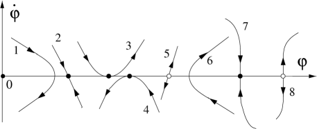
Figure 1: Possible phase curves in the neighborhood of the $\varphi-$axis. Only on the curves 1 and 6, the system crosses the $\varphi$ axis. Curves 2, 3, 4 and 7 have an attractor as a shared point with the $\varphi$ axis, whereas curves 5 and 8 have a repulsor. These attractors and repulsors can be fixed-point solutions or singularities.

Therefore the system can pass the $\varphi$ axis only if the point of intersection is a turning point (curves 1 and 6 on Fig 1). Otherwise the crossing is a fixed point (or a singularity). If there is a smooth phase curve on which the system pass through the $\varphi$ axis, then in a sufficiently small neighborhood of the turning point we have $\left(\varphi-\varphi_{c}\right)\sim\dot{\varphi}^{2n}\sim X^{n}$ where $n\geq 1$. Restricted to this curve, the function $Xp_{,X}(\varphi,X)$ depends only on $X$ and in the absence of a branching point the sign of this function above and below the $\varphi$ axis is the same. Then it follows from the formula (III.2) that the system cannot change the sign of $\left(w+1\right)$ while crossing the $\varphi$ axis.

If a smooth phase curve does not cross but touches the $\varphi$ axis at a point $\varphi_{c}$ (see Fig. 1, trajectories 3 and 4), then the following asymptotic holds: $\dot{\varphi}\sim\left(\varphi-\varphi_{c}\right)^{2n}$, where $n\geq 1$. Let us find the time needed for the system to reach the tangent point $(\varphi_{c},0)$ in this case. We have

$$t\equiv\int_{\varphi_{in}}^{\varphi_{c}}\frac{d\varphi}{\dot{\varphi}(\varphi)}\sim\int_{\varphi_{in}}^{\varphi_{c}}\frac{d\varphi}{\left(\varphi-\varphi_{c}\right)^{2n}},$$ (III.9)

where $\varphi_{in}$ is a starting point on the phase curve. The last integral is obviously divergent. Therefore the system cannot reach the tangent point in a finite time

Finally, we come to the conclusion that in the framework under consideration it is impossible to build a model with the desirable transition through the points $X_{c}=0$.

III.2 Transition at points $\Psi_{c}$: $p_{,X}(\Psi_{c})=0$, $\varepsilon_{,X}(\Psi_{c})\neq 0$, $X_{c}\neq 0$

In the neighborhood of a point $\Psi_{c}$, at which the condition $\varepsilon_{,X}(\Psi_{c})\neq 0$ holds, one can find a function $\dot{\varphi}_{c}(\varphi_{c})$: $p_{,X}\left[\varphi_{c},\dot{\varphi}_{c}(\varphi_{c})\right]=0$. This follows from the theorem about the implicit function. One would anticipate that on the phase curves intersecting the curve $\dot{\varphi}_{c}(\varphi_{c})$ the state of the dark energy changes to the phantom one (or vise versa). Let us express $p_{,X}$ from Eq. (III.2) and substitute it into formula (II.14) for the sound speed of perturbations:

$$c_{s}^{2}=\frac{(w+1)\varepsilon}{2X\varepsilon_{,X}}.$$ (III.10)

For the stability with respect to the general metric and matter perturbations the condition $c_{s}^{2}\geq 0$ is necessary (see Perturbations ). Indeed the increment of instability is inversely proportional to the wavelength of the perturbations, and hence the background models for that $c_{s}^{2}<0$ are violently unstable and do not have any physical significance. Because of the continuity of $\varepsilon_{,X}$, there exists a neighborhood of the point $\Psi_{c}$ where $\varepsilon_{,X}\neq 0$. Therefore, from the above expression for the sound speed (III.10) it follows that if $\left(w+1\right)$ change a sign then $c_{s}^{2}$ should change a sign as well. If this is the case, then the trajectories, realizing the transition, violate the stability condition $c_{s}^{2}\geq 0$. Therefore the model of the transition is not realistic.

III.3 Transition at points $\Psi_{c}$: $p_{,X}(\Psi_{c})=0$, $\varepsilon_{,X}(\Psi_{c})=0$, $X_{c}\neq 0$

As we have already mentioned at the beginning of this section, the points $\Psi_{c}$ generally form the curves in the phase space $(\varphi,\dot{\varphi})$. The subclass of the points $\Psi_{c}$, which we are going to consider in this subsection, is generally a collection of the isolated points given by the solutions of the system,

$$p_{,X}(\varphi,\dot{\varphi})=0, \varepsilon_{,X}(\varphi,\dot{\varphi})=0.$$ (III.11)

Only for specific models, the solutions of this system are not isolated points. An example when these solutions form a line is considered in section IV. Usually the phase curves passing through the isolated points build a set of the zero measure. Therefore it is physically implausible to observe the processes realized on these solutions. The only reason to study the behaviour of the system around these points is their singular character. The point is that the equation of motion (II.13) is not solved with respect to the highest derivatives at this points. In such points there can be more than one phase curve passing through each point. Moreover, the set of solutions $\varphi(t)$, which pass through $\Psi_{c}$ with different $\ddot{\varphi}$, could have a non-zero measure. On the other hand, the equation of motion does not necessarily have a solution $\varphi(t)$ such that $(\varphi(t_{c}),\dot{\varphi}(t_{c}))=\Psi_{c}$ at some moment of time $t_{c}$, or there exists the desirable solution $\varphi(t)$ but it does not possess the second derivative with respect to time at the point $\Psi_{c}$. Below we will analyze the behavior of the phase curves in the neighborhoods of the points $\Psi_{c}$.

The equation of motion (II.13) can be rewritten as a system of two differential equations of the first order:

$$\frac{d\dot{\varphi}}{dt}=-\dot{\varphi}\frac{p_{,X}}{\varepsilon_{,X}}\sqrt{3\varepsilon}-\frac{\varepsilon_{,\varphi}}{\varepsilon_{,X}},$$ (III.12)

$$\frac{d\varphi}{dt}=\dot{\varphi}.$$

The phase curves of this dynamical system are given by the following differential equation:

$$\frac{d\dot{\varphi}}{d\varphi}=-\frac{\dot{\varphi}p_{,X}\sqrt{3\varepsilon}+\varepsilon_{,\varphi}}{\dot{\varphi}\varepsilon_{,X}}.$$ (III.13)

This equation follows from the system (III.12) and therefore all phase curves corresponding to the integral curves of system (III.12) are integral curves of the differential equation (III.13). But the reverse statement is false, so each integral curve of Eq. (III.13) does not necessarily correspond to a solution $\varphi(t)$ of the equation of motion (or of the system (III.12)). In the neighborhoods of the points where $\varepsilon_{,X}\neq 0$, it is convenient to introduce a new auxiliary time variable $\tau$ defined by

$$dt\equiv\varepsilon_{,X}d\tau.$$ (III.14)

The system (III.12) is equivalent to the $\tau$ system:

$$\frac{d\dot{\varphi}}{d\tau}=-\dot{\varphi}p_{,X}\sqrt{3\varepsilon}-\varepsilon_{,\varphi},$$ (III.15)

$$\frac{d\varphi}{d\tau}=\dot{\varphi}\varepsilon_{,X}.$$

The auxiliary time variable $\tau$ change the direction if $\varepsilon_{,X}$ change the sign. Note that the system (III.15) always possesses the same phase curves as the equation of motion (III.12).

In the case under consideration we have $\dot{\varphi}_{c}\neq 0$ and from the formula

$$\frac{d\dot{\varphi}}{d\varphi}=\frac{\ddot{\varphi}}{\dot{\varphi}}$$ (III.16)

we infer that $d\dot{\varphi}/d\varphi(t_{c})$ should be finite, if $\ddot{\varphi}(t_{c})$ is finite. As one can see from the equation determining the phase curves (III.13), in order to obtain a finite $d\dot{\varphi}/d\varphi(t_{c})$ it is necessary that at least $\varepsilon_{,\varphi}(\Psi_{c})=0$. In the case if $\varepsilon_{,\varphi}(\Psi_{c})\neq 0$, the solution $\varphi(t)$ does not possess the second $t$ derivative at the point $t_{c}$. Usually this can be seen as unphysical situation. But nevertheless this does not necessarily lead to the unphysical incontinuity in the observed quantities $\varepsilon,$ $p$, $H$, and $\varphi$, $\dot{\varphi}$. One may probably face problems with the stability of such solutions, but let us first of all investigate the behavior of the phase curves in the case $\varepsilon_{,\varphi}(\Psi_{c})\neq 0$. From Eq. (III.13), we obtain $d\varphi/d\dot{\varphi}=0$ at $\Psi_{c}$. Further we can parameterize the phase curve as $\varphi=\varphi(\dot{\varphi})$ and bring the equation for phase curves (III.13) to the form

$$\frac{d\varphi}{d\dot{\varphi}}=\varepsilon_{,X}(\varphi,\dot{\varphi})F(\varphi,\dot{\varphi}),$$ (III.17)

where we denote

$$F(\varphi,\dot{\varphi})\equiv-\frac{\dot{\varphi}}{\dot{\varphi}p_{,X}\sqrt{3\varepsilon}+\varepsilon_{,\varphi}}.$$ (III.18)

If, as we have assumed, $\varepsilon_{,\varphi}(\Psi_{c})\neq 0$ and $\varepsilon(\Psi_{c})\neq 0$, then $F(\varphi,\dot{\varphi})$ is differentiable in the neighborhood of the point $\Psi_{c}$ and $F(\Psi_{c})=-\dot{\varphi}/\varepsilon_{,\varphi}$. For the second $\dot{\varphi}$ derivative at the point $\Psi_{c}$, one obtains

$$\frac{d^{2}\varphi}{d^{2}\dot{\varphi}}=-\frac{\dot{\varphi}^{2}}{\varepsilon_{,\varphi}}\varepsilon_{,XX}.$$ (III.19)

That is why the point $\Psi_{c}$ is a minimum or a maximum for the function $\varphi(\dot{\varphi})$. In this case $\Psi_{c}$ is such an exceptional point on the phase plot, where the solution $\varphi(t)$ cannot have continuous $\dot{\varphi}(t)$ and the phase curve terminates (see points $\xi$ in Figs. 2 and 3). This happens because the direction of the phase flow is preserved in the neighborhood of $\Psi_{c}$. If $\varepsilon_{,XX}(\Psi_{c})=0$, then one can find the third $\dot{\varphi}$ derivative of $\varphi(\dot{\varphi})$ at the point $\Psi_{c}$:

$$\frac{d^{3}\varphi}{d^{3}\dot{\varphi}}=-\frac{\dot{\varphi}^{3}}{\varepsilon_{,\varphi}}\varepsilon_{,XXX}.$$ (III.20)

In this case there can exist a continuous solution $\varphi(t)$ such that $(\varphi(t_{c}),\dot{\varphi}(t_{c}))=\Psi_{c}$ at some moment of time $t_{c}$ and the only bad thing happening in this point is that $\ddot{\varphi}(t_{c})$ does not exist. Let us now investigate what happens with the equation of state at this point of time. Differentiating both sides of the definition (II.7) of $w$ yields at $t_{c}$

$$\dot{w}_{c}=\left[\frac{\dot{\varphi}}{\varepsilon}\left(p_{,\varphi}-c_{s}^{2}\varepsilon_{,\varphi}\right)\right]_{c},$$ (III.21)

where we have used the equation of motion (II.13) at the point $t_{c}$ and the definition (II.14) of $c_{s}^{2}$. Applying the l’Hôpital rule for the $c_{s}^{2}(t_{c})=\lim\limits_{t\rightarrow t_{c}}p_{,X}/\varepsilon_{,X}$, we find that $c_{s}^{2}(t_{c})=0$. Moreover, using the l’Hôpital rule for the derivative of $c_{s}^{2}$ at the point $\Psi_{c}$, one can find that $dc_{s}^{2}/d\dot{\varphi}\sim p_{,\varphi}/\varepsilon_{,\varphi}$. Thus, if $p_{,\varphi}\neq 0$ the transition could occur but it changes a sign of the sound speed $c_{s}^{2}$. Therefore, if the stability criteria are applicable to this case, then the transition leads to instability.

The necessary condition for the existence of $\ddot{\varphi}$ during the transition is

$$\varepsilon_{,\varphi}(\Psi_{c})=2X_{c}p_{,X\varphi}(\Psi_{c})-p_{,\varphi}(\Psi_{c})=0.$$ (III.22)

This condition drastically reduces the set of the points $\Psi_{c}$, where the transition is possible. Namely, they are the critical points of the function $\varepsilon(\varphi,X)$ and, on the other hand, they are the fixed points of the auxiliary $\tau$ system (III.15). These fixed points are additional to the fixed points of the system (III.12) defined by $\dot{\varphi}=0$ , $\varepsilon_{,\varphi}(\varphi,0)=0$, and $\varepsilon_{,X}(\varphi,0)\neq 0$. From now on, we will consider only those points $\Psi_{c}^{+}$ where the condition (III.22) holds. From the relation (III.22), it follows that if $p_{,\varphi}(\varphi_{c},X_{c})=0$ then $p_{,X\varphi}(\varphi_{c},X_{c})=0$. Otherwise $X_{c}=0$, and as we have already seen the transition cannot happen via the points $X_{c}=0$. Note that if $p_{,\varphi}(\Psi_{c}^{+})=0$, then the points $\Psi_{c}^{+}$ are common critical points of the pressure $p(\varphi,\dot{\varphi})$, energy density $\varepsilon(\varphi,\dot{\varphi})$, and $p_{,X}(\varphi,\dot{\varphi})$. From condition (III.22) follows that points $\Psi_{c}^{+}$ are singular points of Eq. (III.13). In such points there can be more than one phase curve passing through this point. Moreover, as we have already mentioned, the set of solutions $\varphi(t)$, which pass through $\Psi_{c}^{+}$ with different $\ddot{\varphi}$, could have a nonzero measure. For example, if $\Psi_{c}^{+}$ were a nodal point (see Fig. 4), there would be a continuous amount of the solutions passing through this point and therefore there would be a continuous amount of solutions on which the transition could occur.

Let us investigate the type of the singular points $\Psi_{c}^{+}$. This will tell us about the amount of the solutions $\varphi(t)$ on which the transition is possible and their stability. For this analysis, one can use the technique described, for example, in Stepanov , and consider the integral curves of the equation (III.13). Here we proceed with this analysis in a more convenient way, namely, using the auxiliary $\tau$ system (III.15). It is convenient because for this system the singular points $\Psi_{c}^{+}$ are usual fixed points. As we have already mentioned, both systems have the same phase curves and therefore the analysis to perform is also applicable to the phase curves of the system (III.12). The only thing we should not forget is the difference in the directions of the phase flows of these systems. If $\varepsilon(\Psi_{c}^{+})\neq 0$, then one can linearize the right-hand side of the $\tau$ system in the neighborhood of a point $\Psi_{c}^{+}$: $(\varphi_{c}^{+}+\delta\varphi,\dot{\varphi}_{c}^{+}+\delta\dot{\varphi})$. The linearized $\tau$ system (III.15) is

$$\frac{d}{d\tau}\mathbf{V}=\mathbf{AV},$$ (III.23)

where we denote

$$\mathbf{V=\left(\mathbf{\begin{array}[]{c}\delta\varphi\\ \delta\dot{\varphi}\end{array}}\right)}, \mathbf{A=\left(\begin{array}[]{cc}a&b\\ c&g\end{array}\right)},$$ (III.28)

and elements of the matrix $\mathbf{A}$ are given by the formulas

$$a=\varepsilon_{,X\varphi}\dot{\varphi},$$ (III.29)

$$b=2X\varepsilon_{,XX},$$

$$c=-\left(3H\dot{\varphi}p_{,X\varphi}+\varepsilon_{,\varphi\varphi}\right),$$

$$g=-\varepsilon_{,X\varphi}\dot{\varphi},$$

where all quantities are calculated at $\Psi_{c}^{+}$. Here we have used the Friedmann equation (II.10). If $\Psi_{c}^{+}$ is an isolated fixed point of the $\tau$ system (III.15) (or equivalently the singular point of system (III.12)), then the following condition holds

$$\det\mathbf{A}=ag-bc\neq 0.$$ (III.30)

The type of the fixed point depends on the eigenvalues $\lambda$ of the matrix $\mathbf{A}$ (for details see, for example, Pontryagin ). In the case under consideration $a=-g$ and therefore we have

$$\lambda^{2}=bc+a^{2}=-\det\mathbf{A}.$$ (III.31)

If $bc+a^{2}>0$, then eigenvalues $\lambda$ are real and of the opposite signs. In accordance with the classification of the singular points, $\Psi_{c}^{+}$ is a saddle point (see Fig. 2). Therefore the transition is absolutely unstable; there are only two solutions $\varphi(t)$ on which the transition is allowed to occur.

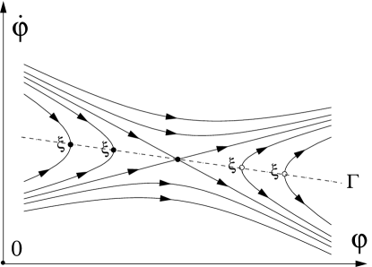
Figure 2: Phase curves in the neighborhood of the singular point $\Psi_{c}^{+}$ are plotted for the case of the real $\lambda$. At the points $\xi$, the solutions $\varphi(t)$ do not exist. These points together with $\Psi_{c}^{+}$ form the curve $\Gamma$ on which $\varepsilon_{,X}(\Gamma)=0$.

If $bc+a^{2}<0$ then $\lambda$ are pure imaginary. Here the situation is a little bit more complicated: In accordance with Stepanov , this fixed point of a nonlinear system can be either a focus or a center. In these cases, as one can see from Fig. 3, there no solutions $\varphi(t)$ passing through the point $\Psi_{c}^{+}$. Therefore, from now on we will consider only the first case - real $\lambda$ of the opposite signs.

Figure 3: Phase curves in the neighborhood of the singular point $\Psi_{c}^{+}$ are plotted for the case of the pure imaginary $\lambda$. Here we assume that the singular point is a focus.

Figure 4: If $\mathbf{A}$ had the eigenvalues $\lambda_{1}=\lambda_{2}$, then the singular point $\Psi_{c}^{+}$ would be a nodal point and there would be a continuous set of trajectories passing through it. To illustrate this we plot here the phase curves in the particular case of a degenerate nodal point. The form of the equation of motion (II.13) excludes such types of singular points and therefore prevents the possibility of such transitions.

It is convenient to rewrite the expression for $\lambda$ into a simpler form. Differentiating the continuity equation (II.11) yields

$$\ddot{\varepsilon}_{c}=-3H_{c}\dot{p}_{c}.$$ (III.32)

Remember that the index $c$ denotes quantities taken at $t_{c}$ or in this subsection at $\Psi_{c}^{+}$. Differentiating the pressure $p$ as a composite function, we have $\dot{p}=p_{,\varphi}\dot{\varphi}+p_{,X}\dot{X}$. Assuming that $\ddot{\varphi}_{c}$ is finite, we obtain that $\dot{p}_{c}=p_{,\varphi}^{c}\dot{\varphi}_{c}$. Thus the formula for $\ddot{\varepsilon}_{c}$ is

$$\ddot{\varepsilon}_{c}=-3H_{c}p_{,\varphi}^{c}\dot{\varphi}_{c}.$$ (III.33)

Using the condition (III.22) and the last equation, we bring the element $c$ of the matrix $\mathbf{A}$ to the following form:

$$c=-\varepsilon_{,\varphi\varphi}^{c}+\frac{\ddot{\varepsilon}_{c}}{2X_{c}}.$$ (III.34)

This relation allows one to rewrite the formula (III.31) as follows:

$$\lambda^{2}=2X_{c}\left(\left(\varepsilon_{,X\varphi}^{c}\right)^{2}-\varepsilon_{,\varphi\varphi}^{c}\varepsilon_{,XX}^{c}\right)+\ddot{\varepsilon}_{c}\varepsilon_{,XX}^{c}.$$ (III.35)

Here it is interesting to note that the expression $\varepsilon_{,\varphi\varphi}^{c}\varepsilon_{,XX}^{c}-\left(\varepsilon_{,X\varphi}^{c}\right)^{2}$ from the previous formula is the determinant of the quadratic form arising in the Taylor set of $\varepsilon$ in the neighborhood of the critical point $\Psi_{c}^{+}$. If this determinant is positive, then the function $\varepsilon(\varphi,X)$ has either a minimum or a maximum at point $\Psi_{c}^{+}$. Otherwise there is either one curve of constant energy density $\varepsilon(\textrm{curve})=\varepsilon(\Psi_{c}^{+})$ with a singular turning point at $\Psi_{c}^{+}$ in the neighborhood of $\Psi_{c}^{+}$ ore two intersecting at $\Psi_{c}^{+}$ curves of constant $\varepsilon$ (see Nikolsky ) . On the other hand, differentiating $\varepsilon$ as a composite function we find

$$\ddot{\varepsilon}_{c}=2X_{c}\left(\varepsilon_{,\varphi\varphi}^{c}+2\varepsilon_{,X\varphi}^{c}\ddot{\varphi}_{c}+\varepsilon_{,XX}^{c}\ddot{\varphi}_{c}^{2}\right).$$ (III.36)

Substituting this relation into the previous formula (III.35) for $\lambda$ yields

$$\lambda^{2}=2X_{c}\left(\varepsilon_{,XX}^{c}\ddot{\varphi}_{c}+\varepsilon_{,X\varphi}^{c}\right)^{2}.$$ (III.37)

This formula provides the relation between $\ddot{\varphi}_{c}$ at the moment of transition and $\lambda$. Note that $\lambda$ depends on $\ddot{\varphi}_{c}$ only in the case when $\varepsilon_{,XX}(t_{c})\equiv 2X_{c}p_{,XXX}(t_{c})\neq 0$. Moreover, comparing formulas (III.33) and (III.36) for $\ddot{\varepsilon}_{c}$, one can obtain the equation on $\ddot{\varphi}_{c}$:

$$\varepsilon_{,XX}^{c}\dot{\varphi}_{c}\ddot{\varphi}_{c}^{2}+2\varepsilon_{,X\varphi}^{c}\dot{\varphi}_{c}\ddot{\varphi}_{c}+\dot{\varphi}_{c}\varepsilon_{,\varphi\varphi}^{c}+3H_{c}p_{,\varphi}^{c}=0.$$ (III.38)

This equation is solvable in real numbers if the discriminant is positive. As one can prove, the discriminant is exactly the $4\lambda^{2}$ and therefore positive if we consider the saddle point. The same can be seen from relation (III.37) as well.

Let us denote the positive and negative eigenvalues and the corresponding eigenvectors of $\mathbf{A}$ as $\lambda_{+}$, $\lambda_{-}=-\lambda_{+}$ and $\mathbf{a}_{+}$, $\mathbf{a}_{-}$, respectively.

If $b\neq 0$ ( or equivalently $\varepsilon_{,XX}^{c}\neq 0$), then the eigenvectors can be chosen as $\mathbf{a}_{+}=(1,(\lambda_{+}-a)/b)$ and $\mathbf{a}_{-}=(1,-(\lambda_{+}+a)/b)$. Therefore the separatrices forming the saddle are

$$\delta\dot{\varphi}_{+}=\frac{\lambda_{+}-a}{b}\delta\varphi \delta\dot{\varphi}_{-}=-\frac{\lambda_{+}+a}{b}\delta\varphi.$$ and

The general solution for the phase curves in the neighborhood of $\Psi_{c}^{+}$ is

$$\left(\delta\dot{\varphi}-\frac{\lambda_{+}-a}{b}\delta\varphi\right)\left(\delta\dot{\varphi}+\frac{\lambda_{+}+a}{b}\delta\varphi\right)=const.$$ (III.39)

If $b=0$ and additionally $a>0$, then we have $\lambda_{+}=a=\varepsilon_{,X\varphi}\dot{\varphi}$, and one can choose the eigenvectors as $\mathbf{a}_{+}=(1,c/2a)$ and $\mathbf{a}_{-}=(0,1)$ . For a negative $a$, one can obtain the eigenvectors and eigenvalues by changing $\lambda_{+}\leftrightarrow\lambda_{-}$ and $\mathbf{a}_{+}\leftrightarrow\mathbf{a}_{-}$. The separatrices then read

$$\delta\varphi=0 \delta\dot{\varphi}=\frac{c}{2a}\delta\varphi.$$ and

Thus, similarly to the previous case, the phase curves are given by

$$\delta\varphi\left(\delta\dot{\varphi}-\frac{c}{2a}\delta\varphi\right)=const.$$ (III.40)

As we have already mentioned from the formula $d\dot{\varphi}/d\varphi$$=\ddot{\varphi}/\dot{\varphi}$, follows that, at the points where the phase curves are parallel to the $\dot{\varphi}$ axis and where $\dot{\varphi}\neq 0$, the second $t$ derivative of the field does not exist. If we look at the equations (III.39) and (III.40) providing the phase curves in the neighborhood of $\Psi_{c}^{+}$, then we find that in the first case (when $\varepsilon_{,XX}^{c}\neq 0$) the phase curves lying on the right- and left- hand sides of both separatrices should have a point $\xi$ where they are parallel to the $\dot{\varphi}$ axis (see Fig. 2). Therefore each of these phase curves consists of two solutions of the equation of motion (II.13) and the exceptional point $\xi$ where the solution $\varphi(t)$ does not exist. The same statement holds in the case of the pure imaginary $\lambda$ (see Fig. 3). This behavior is not forbidden because, as one can easily prove, the exceptional points $\xi$ lie exactly on the curve $\Gamma$ on which $\varepsilon_{,X}(\Gamma)=0$ and the equation of motion is not solved with respect to the highest derivatives. Note that we have already assumed $\lambda\neq 0$, and from this condition it follows that $\varepsilon_{,XX}^{c}$ and $\varepsilon_{,X\varphi}^{c}$ cannot vanish simultaneously. Therefore in the neighborhood of the point $\Psi_{c}^{+}$ there exists an implicit function $\dot{\varphi}(\varphi)$ (or $\varphi(\dot{\varphi})$) and its plot gives the above-mentioned curve $\Gamma$ on which $\varepsilon_{,X}(\Gamma)=0$. In the case $\varepsilon_{,XX}^{c}=0$, the separatrix $\delta\varphi=0$ locally coincides with $\Gamma$, and therefore, this integral curve of Eq. (III.13) does not correspond to any solution $\varphi(t)$ of the equation of motion. Nevertheless, in virtue of the existence theorem, all phase curves obtained in the neighborhood of the separatrix $\delta\varphi=0$ correspond to the solutions of the equation of motion. Moreover, if $\varepsilon_{,XX}^{c}=0$ and $p_{,X\varphi}^{c}\neq 0$ then the curves on which $p_{,X}=0$ and $\varepsilon_{,X}=0$ locally coincide with each other and with the curve $\delta\varphi=0$. The only phase curve intersecting the curve $\delta\varphi=0$ at $\Psi_{c}^{+}$ is the second separatrix $\delta\dot{\varphi}=c\delta\varphi/2a$. Thus the only solution $\varphi(t)$ on which the transition happens in the neighborhood of $\Psi_{c}^{+}$ corresponds to the separatrix $\delta\dot{\varphi}=c\delta\varphi/2a$. This can also be seen from the equation (III.38) which has only one root $\ddot{\varphi}_{c}$ in this case. In the Sec. (IV) we will illustrate this with a numerical example (see Fig. 5).

It is worthwhile to discuss cases which fall out from the consideration made above. We have assumed that $\lambda\neq 0$ and therefore $\Psi_{c}^{+}$ is an isolated singular point of Eq. (III.13). The most natural possibilities to drop out this condition are $\varepsilon_{,X\varphi}^{c}=0$ and either $\varepsilon_{,XX}^{c}=0$ or $\dot{\varphi}_{c}3H_{c}p_{,X\varphi}^{c}+\varepsilon_{,\varphi\varphi}^{c}=0$. In the first case $\Psi_{c}^{+}$ is a critical point not only of the function $\varepsilon$ but of the function $\varepsilon_{,X}$ as well. This can be obtained either for a very special kind of function $p$ namely, such that $p_{,X}=0$, $p_{,XX}=0$, $p_{,XXX}=0$, and $\left[p-4X^{2}p_{,XX}\right]_{,\varphi}=0$ at $\Psi_{c}^{+}$ or imposing the condition that the point $\Psi_{c}^{+}$ is a critical point not only of $p$ but also of the functions $p_{,X}$ and $p_{,XX}$: $p_{,X}=0$, $p_{,\varphi}=0$, $p_{,XX}=0,$ $p_{,X\varphi}=0$, $p_{,XX\phi}=0$, and finally $p_{,XXX}=0$ at $\Psi_{c}^{+}$. In the second case $\Psi_{c}^{+}$ is a common critical point for the functions $\varepsilon$ and $\varepsilon_{,\varphi}$. In terms of $p$, this condition is as follows: $p_{,X}=0$, $p_{,\varphi}=0$, $p_{,X\varphi}=0$, $p_{,XX}=0,$ $p_{,\varphi\varphi}=0$, $p_{,XX\varphi}=0$, and finally $p_{,X\varphi\varphi}=0$ at $\Psi_{c}^{+}$ . Thus, the point $\Psi_{c}^{+}$ is a common critical point of $p$, $p_{,X}$ and $p_{,X\varphi}$. Of course, the analysis performed above does not work in the case if the function $p(\varphi,X)$ does not have a sufficient amount of derivatives. It is clear that all these cases are not general.

Let us sum up the results obtained in this section. In the general case of linearizable functions $\varepsilon_{,X}$, $\varepsilon_{,\varphi},$ and $p_{,X}$, the considered transitions either occur through the points $\Psi_{c}^{+}$, where $p_{,X}=0$, $\varepsilon_{,X}=0$, $\varepsilon_{,\varphi}=0$, and

$$\dot{\varphi}\left[\left(\varepsilon_{,X\varphi}^{2}-\varepsilon_{,\varphi\varphi}\varepsilon_{,XX}\right)\dot{\varphi}-3H\varepsilon_{,XX}p_{,\varphi}\right]>0$$

or lead to an unacceptable instability with respect to the cosmological perturbations of the background. The points $\Psi_{c}^{+}$ are critical points of the energy density and are the singular points of the equation of motion of the field $\varphi$ as well. These singular points are saddle points and the transition is realized by the repulsive separatrix solutions, which form the saddle. Therefore the measure of these solutions is zero in the set of trajectories and the dynamical transitions from the states where $w>-1$ to $w<-1$ or vise versa are physically implausible.

IV Lagrangians linear in $X$

The simplest class of models, for that one could anticipate the existence of dynamical transitions, is the dark energy described by Lagrangians $p(\varphi,X)$ linear in $X$:

$$p(\varphi,X)=KX-\frac{1}{2}V\equiv\frac{1}{2}\left(K(\varphi)\nabla_{\mu}\varphi\nabla^{\mu}\varphi-V(\varphi)\right).$$ (IV.1)

In the isotropic and homogeneous Friedmann universe, the Lagrangian is then

$$p(\varphi,\dot{\varphi})=\frac{1}{2}\left(K(\varphi)\dot{\varphi}^{2}-V(\varphi)\right).$$ (IV.2)

For these models, we always have $c_{s}^{2}=1$ and therefore, as follows from our analysis, the transitions could occur only through the points where $\varepsilon_{,X}=0$. The energy density for this model is

$$\varepsilon(\varphi,\dot{\varphi})=\frac{1}{2}\left(K(\varphi)\dot{\varphi}^{2}+V(\varphi)\right).$$ (IV.3)

If one takes $K(\varphi)\equiv 1$, then the Lagrangian (IV.2) is the usual Lagrangian density for scalar field with a self-interaction. If we take $K(\varphi)\equiv-1$, then we obtain the so-called “Phantom field” from Caldwell Manace and Hoffman . The case $K(\varphi)>0$ corresponds to $w\geq-1$, whereas $K(\varphi)<0$ corresponds to $w\leq-1$. The equation of motion (II.13) takes in our case the following form:

$$\ddot{\varphi}K+\dot{\varphi}K\sqrt{3\varepsilon}+\varepsilon_{,\varphi}=0.$$ (IV.4)

While the equation determining the phase curves (III.13) reads in this particular case

$$\frac{d\dot{\varphi}}{d\varphi}+\sqrt{3\varepsilon}+\frac{1}{\dot{\varphi}K}\varepsilon_{,\varphi}=0.$$ (IV.5)

If $K(\varphi)$ is a sign-preserving function, one can redefine field $\varphi$: $\sqrt{\left|K(\varphi)\right|}d\varphi=d\phi$ (see also Ref. Liddle ). The equation of motion for the new field $\phi$ can be obtained from Eq. (IV.4), through the formal substitutions $\varphi\rightarrow\phi$, $V(\varphi)\rightarrow\tilde{V}(\phi)\equiv V(\varphi(\phi))$, and $K(\varphi)\rightarrow\pm 1$, where the upper sign corresponds to a positive $K(\varphi)$ and the lower one to a negative $K(\varphi)$. After these substitutions, the equation of motion (IV.4) looks more conventionally

$$\ddot{\phi}+\dot{\phi}\sqrt{\frac{3}{2}\left(\pm\dot{\phi}^{2}+\tilde{V}(\phi)\right)}\pm\frac{1}{2}\left(\frac{\partial\tilde{V}(\phi)}{\partial\phi}\right)=0.$$ (IV.6)

Moreover, this equations is easier to dial with, because one can visualize the dynamic determined by it, as 1D classical mechanics of a point particle in a potential $\pm\tilde{V}(\phi)/2$ with a little bit unusual friction force. If we were able to solve the equation of motion (IV.6) for all possible $\tilde{V}(\phi)$ and initial data, we could solve the problem of cosmological evolution for all linear in $X$ Lagrangians with sign-preserving $K(\varphi)$.

If the function $K(\varphi)$ is not sign-preserving, then at first sight it seems that the dark energy, described by such a Lagrangian, can realize the desirable transition. The function $K(\varphi)$ generally can change the sign in two ways: In the continuous one, then the function $K(\varphi)$ takes the value zero for some values of field $\varphi$ or in a discontinuous polelike way.

IV.1 Linearizable $K(\varphi)$

Without loss of generality, one can assume that $K(0)\equiv K_{c}=0$, $K(\varphi)<0$ for the negative values of $\varphi$ and $K(\varphi)>0$ for $\varphi>0$. The line $\varphi=0$ on the phase plot $(\varphi,\dot{\varphi})$ we will call the “critical” line for the given class of Lagrangians. The phantom states $(\varphi,\dot{\varphi})$ of the scalar field lie on the left-hand side, while the usual states with $w\geq-1$ are on the right-hand side of the critical line. If there exists a solution $\varphi(t)$ whose phase curve passes through the “critical” line, then the dark energy can change the sign of $\left(w+1\right)$ during the cosmological evolution. From now on, we will investigate the behavior of the phase curves of the system in the neighborhood of the critical line.

First of all, it is worth considering the functions $K(\varphi)$ such that $K_{c}^{\prime}>0$ (here we have denoted $K{}_{,\varphi}(0)\equiv K{}_{c}^{\prime}$), because in this case we can directly apply the outcome of our previous analysis made in the Sec. III.1. Condition (III.22) is for the linear in $X$ Lagrangians as follows:

$$\dot{\varphi}_{c}^{2}K_{c}^{\prime}+V_{c}^{\prime}=0.$$ (IV.7)

As we have already assumed $K_{c}^{\prime}>0$, therefore, if $V_{c}^{\prime}>0$, then, as follows from condition (IV.7), there are no twice differentiable solutions $\varphi(t)$ whose phase curves would intersect or touch the critical line. Further (see formula (IV.15) and below) we will show that, for the linear in $X$ Lagrangians, condition (III.22) (or in our case condition (IV.7) is necessary not only for the existence of the second $t$ derivative $\ddot{\varphi}$ at the point of intersection with the critical line but for the existence of a solution $\varphi(t)$ at this point as well. Thus, we come to the conclusion that, if $V_{c}^{\prime}>0$, then two regions $\varphi<0$, and $\varphi>0$ on the phase plot are not connected by any phase curves and accordingly the dark energy does not change the sign of $\left(w+1\right)$ during the cosmological evolution.

In the case $V_{c}^{\prime}<0$, we can solve Eq. (IV.7) with respect to $\dot{\varphi}_{c}$ :

$$\dot{\varphi}_{c}=u_{\pm}\equiv\pm\sqrt{-\frac{V_{c}^{\prime}}{K_{c}^{\prime}}}.$$ (IV.8)

The phase curves, lying in the neighborhoods of the singular points $\Psi_{c}^{+}=(0,u_{\pm})$, are to obtain from the relation (III.40), which gives:

$$\varphi\left(\dot{\varphi}-u_{\pm}-\frac{A_{\pm}}{2}\varphi\right)=const,$$ (IV.9)

where

$$A_{\pm}=-3H_{c}+\frac{V_{c}^{\prime}K_{c}^{\prime\prime}-V_{c}^{\prime\prime}K_{c}^{\prime}}{2u_{\pm}\left(K_{c}^{\prime}\right)^{2}}.$$ (IV.10)

For each singular point $(0,u_{\pm})$, there is a corresponding solution $\varphi_{\pm}(t)$ whose phase curve is the separatrix

$$\dot{\varphi}_{\pm}=u_{\pm}+\frac{A_{\pm}}{2}\varphi,$$ (IV.11)

which intersects the critical line. These phase curves correspond to the $const=0$ in the right-hand side of Eq. (IV.9). Another curve, which corresponds to $const=0$ is $\varphi=0$. As we have already mentioned at the end of the previous subsection, this curve does not correspond to any solutions $\varphi(t)$ of the equation of motion (IV.4).

Considering the phase flow in the neighborhoods of $\Psi_{c}^{+}=(0,u_{\pm})$ (see Fig. 5), we infer that the separatrices $\dot{\varphi}_{\pm}$ are repulsors immediately before they intersect the critical line and attractors after the crossing. Hence, the measure of the initial conditions $(\varphi,\dot{\varphi})$ leading to the transition to phantom field (or vice versa) is zero. In this sense the dark energy cannot change the sign of $K(\varphi)$ (or equivalently the sign of $\left(w+1\right)$) during the cosmological evolution.

The typical behavior of the phase curves in the neighborhood of the singular points $(0,\,u_{\pm})$, for the models under consideration ($K_{c}^{\prime}>0$, $V_{c}^{\prime}<0$), is shown in Fig. 5. Here, as an example, we have plotted the phase curves obtained numerically for a toy model with the Lagrangian density $p=\frac{1}{2}\varphi\dot{\varphi}^{2}-\frac{1}{2}\left(\left(\varphi-1\right)^{2}+\frac{1}{3}\right)$. For this model we have $u_{\pm}=\pm 1$, $A_{+}=-\frac{3}{2}$, and $A_{-}=-\frac{1}{2}$.

Let us now consider such potentials $V(\varphi)$ that $V_{c}^{\prime}=0$. If $K(\varphi)$ is a differentiable function, then, in the case under consideration, the equation of motion (IV.4) obviously has a fixed-point solution $\varphi(t)\equiv 0$ but this solution is not necessarily the unique one. When $V_{c}^{\prime}=0$ and $K_{c}^{\prime}>0$, then, as follows from the condition (III.22), the only value $\dot{\varphi}$, where a phase curve could have coinciding points with the critical line, is $\dot{\varphi}=0$. From the analysis made in Sec. III.1, we have already learned that the transition is impossible in this case. Nevertheless it is worth to showing explicitly how the phase curves look at this case. Taking into consideration only the leading order in the numerator and denominator of Eq.  (IV.5) and assuming that $V_{c}^{\prime\prime}\neq 0$, we obtain

$$\frac{d\dot{\varphi}}{d\varphi}\simeq-\frac{V_{c}^{\prime\prime}}{2\dot{\varphi}K_{c}^{\prime}}.$$ (IV.12)

The solution of this equation, going through the point $(0,0)$ on the phase plot, is

$$\varphi_{s}=-\dot{\varphi}^{2}\left(\frac{K_{c}^{\prime}}{V_{c}^{\prime\prime}}\right).$$ (IV.13)

In Fig. 6 we have plotted the phase curves obtained numerically for a toy model with the Lagrangian density $p=\frac{1}{2}\varphi\dot{\varphi}^{2}-\frac{1}{2}\left(\varphi^{2}+2\right)$. As one can see from Fig. 6, the parabolalike phase curve $\varphi_{s}$, given by the formula (IV.13), is the separatrix going through the fixed-point solution $\varphi(t)\equiv 0$. Moreover, this figure confirms that there are no phase curves intersecting the critical line by finite $\dot{\varphi}$.

Figure 5: The typical behavior of the phase curves in the neighborhood of the critical line where $K(\varphi)=0$ (here $\dot{\varphi}$ axis ) is plotted for the case when $K_{c}^{\prime}>0$ and $V_{c}^{\prime}<0$. Horizontal dashed lines are the analytically obtained separatrices $\dot{\varphi}_{\pm}$ and $(0,u_{\pm})$ are the points of transition.

Figure 6: The typical behavior of the phase curves in the neighborhood of the critical line where $K(\varphi)=0$ (here $\dot{\varphi}$ axis ) is plotted for the case when $K_{c}^{\prime}>0$, $V_{c}^{\prime}=0$, and $V_{c}^{\prime\prime}>0$.

IV.2 General differentiable $K(\varphi)$

The models we are going to discuss below belong to the more general class of models for which the function $K(\varphi)$ has zero of an odd order $2n+1$ (where $n\geq 0$) at $\varphi=0$. For the linear in $X$ Lagrangians, we have $\varepsilon_{,XX}\equiv 0$; therefore, if $n>0$ then $K_{c}^{\prime}=0$ and $\varepsilon_{,\varphi X}^{c}=0$. That is why the general analysis made in the Sec.  III.3 does not work for this case. Therefore it is interesting to investigate on this simple example whether the desired transition could be possible for models not covered by our former analysis. If $K(\varphi)$ is a sufficient many times differentiable function, then for $\left|\varphi\right|\ll 1$ we have

$$K(\varphi)\simeq\frac{K_{c}^{\left(2n+1\right)}}{\left(2n+1\right)!}\varphi^{2n+1},$$ (IV.14)

where $K_{c}^{\left(2n+1\right)}$ is the $(2n+1)$th $\varphi$ derivative of $K$ at $\varphi=0$. If there is a phase curve, crossing the critical line at a finite nonvanishing $\dot{\varphi}_{c}$, then integrating both sides of the equation of motion (IV.4) we obtain

$$\dot{\varphi}_{c}-\dot{\varphi}_{in}=-3\int_{\varphi_{in}}^{0}H(\varphi)d\varphi-\int_{\varphi_{in}}^{0}\frac{\varepsilon_{,\varphi}}{\dot{\varphi}K}d\varphi.$$ (IV.15)

Here $(\varphi_{in},\dot{\varphi}_{in})$ is a point on the phase curve in the neighborhood of the critical line. The first integral on the right-hand side of Eq. (IV.15) is always finite, whereas, as follows from the relation (IV.14), the second integral is definitely divergent, if $\varepsilon_{,\varphi}^{c}\neq 0$. This divergence contradicts to our initial assumption: $\dot{\varphi}_{c}$ - finite. Therefore we again obtain the condition (III.22), which restricts the possible intersection points on the critical line in the sense that in the other points, where the condition does not hold, not only the second derivative $\ddot{\varphi}$ does not exist, but there are no solutions $\varphi(t)$ at all. Moreover, it is clear that the condition (IV.7) is not enough for the existence of the solutions intersecting the critical line. Thus, if the order of $V^{\prime}(\varphi)$ exceeds the order on $\varphi$ of $K^{\prime}(\varphi)$ for $\left|\varphi\right|\ll 1$, then one can neglect $V^{\prime}(\varphi)$ and the integral (IV.15) has the logarithmic divergence (note that we do not consider the points $\dot{\varphi}_{c}=0$ because as we already know the transition does not occur via these points). When the order of $V^{\prime}(\varphi)$ is lower than $K^{\prime}(\varphi)$ (and therefore lower than the order of $K(\varphi)$), we can neglect $\dot{\varphi}^{2}K^{\prime}(\varphi)$ and the integral (IV.15) has a power-low divergence. Finally, if the functions $K^{\prime}(\varphi)$ and $V^{\prime}(\varphi)$ have the same order on $\varphi$ for $\left|\varphi\right|\ll 1$ and are of opposite signs in a sufficient small neighborhood of $\varphi=0$, then one can find an appropriate finite value $\dot{\varphi}_{c}^{2}\neq 0$ for which the divergence on the right-hand side of Eq.  (IV.15) is canceled. One would expect that at this point the phase curves intersect the “critical” line and the dark energy changes the sign of $\left(w+1\right)$. Below, we give the direct calculation of these $\dot{\varphi}_{c}$ and the phase curves in a neighborhood of them. Suppose that the order of the functions $\left(V(\varphi)-V_{c}\right)$ and $K(\varphi)$ is $(2n+1)$ and there exist their derivatives of the order $(2n+2)$. Then for the $\varphi$ derivative of the energy density we have in the neighborhood of the supposed intersection point $(0,\dot{\varphi}_{c})$:

$$\varepsilon_{,\varphi} \simeq\frac{1}{2}\frac{\varphi^{2n}}{\left(2n\right)!}\left[\left(\dot{\varphi}_{c}^{2}K_{c}^{(2n+1)}+V_{c}^{(2n+1)}\right)+2\dot{\varphi}_{c}K_{c}^{(2n+1)}\delta\dot{\varphi}\right.$$

$$+\frac{\varphi}{\left(2n+1\right)}\left.\left(\dot{\varphi}_{c}^{2}K_{c}^{(2n+2)}+V_{c}^{(2n+2)}\right)\right],$$ (IV.16)

whereas the denominator $\dot{\varphi}K(\varphi)$ of the second integral on the right-hand side of Eq. (IV.15) has the order $(2n+1)$ on $\varphi$. The only possibility to get rid of the divergence in the integral under consideration is to assume that the first term in the brackets in the asymptotic (IV.16) for $\varepsilon_{,\varphi}$ is zero. Therefore the possible crossing points are given by

$$\dot{\varphi}_{c}=u_{\pm}=\pm\sqrt{-\frac{V_{c}^{(2n+1)}}{K_{c}^{(2n+1)}}.}$$ (IV.17)

Taking into account only the leading order on $\varphi$ and $\delta\dot{\varphi}$ in the denominator and the numerator of Eq. (IV.5), we obtain differential equation for the phase curves in the neighborhoods of the intersection points $(0,u_{\pm})$:

$$\frac{d\delta\dot{\varphi}}{d\varphi}=A_{\pm}-\left(2n+1\right)\frac{\delta\dot{\varphi}}{\varphi},$$ (IV.18)

where

$$A_{\pm}=-3H_{c}+\frac{K_{c}^{(2n+2)}V_{c}^{\left(2n+1\right)}-K_{c}^{(2n+1)}V_{c}^{\left(2n+2\right)}}{2\left[K_{c}^{(2n+1)}\right]^{2}u_{\pm}}.$$ (IV.19)

The solutions of this equation are given by the formula

$$\left(\delta\dot{\varphi}-\frac{A_{\pm}}{2n+2}\varphi\right)\varphi^{2n+1}=const,$$ (IV.20)

which is a generalization of formula (IV.9). Similarly to the case $n=0$ ($K_{c}^{\prime}>0$) the solutions, on which the transition occurs, have the measure zero in the phase curves set. Therefore we infer that the dynamical transition from the phantom states with $w\leq-1$ to the usual with $w\geq-1$ (or vice versa) is impossible.

Now we would like to mention the models, for which $V^{\prime}(\varphi)$ is one order higher on $\varphi$ than $K^{\prime}(\varphi)$ for small $\varphi$. From the asymptotic expression for $\varepsilon_{,\varphi}$ (IV.16) and the relation, giving the possible values of $\dot{\varphi}_{c}$ (IV.15), we see that the only point on the critical line which could be reached in a finite time is $\dot{\varphi}_{c}=0$. Therefore, as we have seen in Sec. III.1, the transition is impossible. The phase curve going trough the fixed-point solution $\varphi(t)\equiv 0$ is a parabola given by the generalization of Eq. (IV.13) :

$$\varphi\simeq-\dot{\varphi}^{2}\left[\frac{K_{c}^{\left(2n+1\right)}}{V_{c}^{\left(2n+2\right)}}\right].$$ (IV.21)

If $V^{\prime}(\varphi)$ is more than one order higher on $\varphi$ than $K^{\prime}(\varphi)$, then as we have already mentioned $\dot{\varphi}_{c}=0$ and the transition is impossible as well.

IV.3 Pole-like $K(\varphi)$

In this subsection, we briefly consider the case when the function $K(\varphi)$ has a pole of an odd order, so $K\sim\varphi^{-2n-1}$, where $n>0$, for $\left|\varphi\right|\ll 1$. This kind of functions $K(\varphi)$ is often discussed in the literature in connection with the $k-$essence models (see k-Essence ). Let us keep the same notation as in subsection IV.1. The potential $V(\varphi)$ can not have a pole at the point $\varphi=0$, because, if it were the case, either the energy density $\varepsilon$ or the pressure $p$ would be infinite on the critical line. In order to obtain finite values of the energy density $\varepsilon$ and pressure $p$, it is necessary to assume that the system intersects the critical line at $\dot{\varphi}=0$. But, as we have already seen in Sec.  III.1, the dark energy cannot change the the sign of $\left(w+1\right)$ at the points $\dot{\varphi}=0$.

Thus, we have shown that in the particular case of the theories described by the linear in $X$ Lagrangians $p(\varphi,X)=K(\varphi)X-V(\varphi),$ which are differentiable in the neighborhood of $\Psi_{c}^{+}$ ($K(\varphi)$ and $V(\varphi)$ differentiable but not necessary linearizable) the results, obtained for linearizable functions $\varepsilon_{,X}$, $\varepsilon_{,\varphi}$, and $p_{,X}$, hold as well. This gives rise to hope that the same statement is true for the general nonlinear in $X$ Lagrangians as well. Especially we have proven that, if the construction of the linear in $X$ Lagrangian allows the transition, then the transitions always realize on a pair of the phase curves. One phase curve corresponds to the transition from $w>-1$ to $w<-1$ while another one realizes the inverse transition. This pair of phase curves obviously has the measure zero in the set of trajectories of the system. Therefore we infer that the considered transition is physically implausible in this case.

V Scalar dark energy in open and closed universes in the presence of other forms of matter

In the previous sections, we have seen that the desirable transition from $w>-1$ to $w<-1$ is either impossible or dynamically unstable in the case when the scalar dark energy is a dominating source of gravity in the flat Friedmann universe. Let us now investigate whether this statement is true in the presence of other forms of matter and in the cases when the Friedmann universe has open and closed topology.

Following Ref. Perturbations , the effective sound speed $c_{s}$ is given by the same Eq. (II.14) for the flat, open, and closed universes. Therefore, if the dark energy is the dominating source of gravitation (in particular this means that the energy density of the dark energy $\varepsilon\neq 0$ ), then the analysis made in Sec. III.2 is applicable to open and closed universes as well as to the flat universe.

If the dark energy under consideration interacts with ordinary forms of matter only through indirect gravitational-strength couplings, then the equation of motion (II.13) can be written in the following form:

$$\ddot{\varphi}\varepsilon_{,X}+3\dot{\varphi}Hp_{,X}+\varepsilon_{,\varphi}=0,$$ (V.1)

where merely the Hubble parameter depends on the spatial curvature and other forms of matter. This dependence is given by the Friedmann equation:

$$H^{2}+\frac{k}{a^{2}}=\frac{1}{3}\left(\varepsilon+\sum\varepsilon_{i}\right),$$ (V.2)

where $\sum\varepsilon_{i}$ is the total energy density. It is obvious that the points on the plot $(\varphi,\dot{\varphi})$ considered in the most of this paper do not define the whole dynamics of the system anymore and therefore do not define the states of the whole system. The analysis made in Secs. III.1, III.3, and IV leans only on the behavior of the scalar filed $\varphi$ and its first $t$ derivative $\dot{\varphi}$ in the neighborhoods of their selected values, namely, such as where some of the conditions $p_{,X}=0$, $\dot{\varphi}=0$, or $\varepsilon_{,X}=0$ etc. hold. For these conditions, the contributions into the equation of motion (V.1) coming from the other forms of matter and spatial curvature would be of a higher order and therefore are not important for the local behavior of $\varphi$ and the problem as a whole. In fact, the value of the Hubble parameter did not change the qualitative futures of the phase curves considered in Secs. III.1,III.3, and IV. To illustrate this statement, we plot the trajectories of the system $p=\frac{1}{2}\varphi\dot{\varphi}^{2}-\frac{1}{2}\left(\left(\varphi-1\right)^{2}+\frac{1}{3}\right)$ (it is the same system that we considered in previous subsection) in presence of dust matter for various values of the initial energy densities of the dust (see Fig. 7). The only thing that is important is that $H\neq 0$. The universe should not change the expansion to the collapse and the plot of the scale factor $a(t)$ should not have a cusp directly at the time of the transition. Thus, we infer that the most of our analysis is applicable to a more general physical situation of a Friedmann universe filled with various kinds of usual matter, which interact with the dark energy only through indirect gravitational-strength couplings. Moreover, if the interaction between the dark energy field $\varphi$ and other fields does not include coupling to the derivatives $\nabla_{\mu}\varphi$, then the obtained result holds as well.

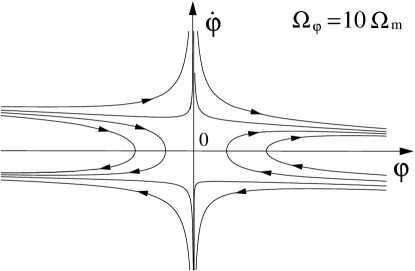
Figure 7: Numerically obtained trajectories of the dark energy described by a Lagrangian linear in $X$ are plotted for the cases $\Omega_{\varphi}=10\Omega_{m}$, $\Omega_{\varphi}=\Omega_{m}$, and $\Omega_{\varphi}=0.1\Omega_{m}$.

VI Conclusions and Discussion

In this paper we have found that the transitions from $w>-1$ to $w<-1$ (or vice versa) of the dark energy described by a general scalar-field Lagrangian $p(\varphi,\nabla_{\mu}\varphi)$ are either unstable with respect to the cosmological perturbations or realized on the trajectories of the measure zero. If the dark energy dominates in the universe, this result is still robust in the presence of other energy components interacting with the dark energy through nonkinetic couplings. In particular, we have shown that, under this assumption about interaction, the dark energy described by Lagrangians linear in $\left(\nabla_{\mu}\varphi\right)^{2}$ cannot yield such transitions even if it is a subdominant source of gravitation.

Let us now discuss the consequences of these results. If further observations confirm the evolution of the dark energy dominating in the universe, from $w\geq-1$ in the close past to $w<-1$ to date, then it is impossible to explain this phenomenon by the classical dynamics given by an effective scalar-field Lagrangian $p(\varphi,\nabla_{\mu}\varphi)$. In fact, the models which allow such transitions have been already proposed (see e.g., Triad ; Xinmin Zhang ; Shtanov and other models from the Ref. Review ) but they incorporate more complicated physics then the classical dynamics of a one scalar field.

If observations reveal that $w<-1$ now and if we disregard the possibility of the transitions, then the energy density of the dark energy should grow rapidly during the expansion of the universe and therefore the coincidence problem becomes even more difficult. Thus, from this point of view the transitions considered in this paper would be rather desirable for the history of the universe. As we have shown, to explain the transition under the minimal assumptions of the nonkinetic interaction of dark energy and other matter one should suppose that the dark energy was subdominating and described by a nonlinear in $\left(\nabla_{\mu}\varphi\right)^{2}$ Lagrangian. Thus, some nonlinear (or probably quantum) physics must be invoked to explain the value $w<-1$ in models with one scalar field.

The second application of our analysis is the problem of the cosmological singularity. To obtain a bounce instead of collapse, the scalar field $\varphi$ must change its equation of state to the phantom one before the bounce and should dominate in the universe at the moment of transition. Otherwise, if the scalar field was subdominant then it is still subdominant after the transition as well, because its energy density decreases during the collapse, while the other nonphantom forms of matter increase their energy densities. The disappearing energy density of $\varphi$ does not affect the gravitational dynamics and therefore does not lead to the bounce. On the other hand, as we have already proved, a dominant scalar field $\varphi$ described by the action without kinetic couplings and higher derivatives cannot smoothly evolve to the phantom with $w<-1$. Therefore we infer that a smooth bounce of the nonclosed Friedmann universe cannot be realized in this framework.

- (1) Ujjaini Alam, Varun Sahni, Tarun Deep Saini, A. A. Starobinsky, preprint astro-ph/0311364.
- (2) Ujjaini Alam, Varun Sahni, A. A. Starobinsky, preprint astro-ph/0403687,.
- (3) S. W. Allen, R. W. Schmidt, H. Ebeling, A. C. Fabian and L. van Speybroeck, preprint astro-ph/0405340.
- (4) S. Perlmutter et al., [Supernova Cosmology Project Collaboration], Astrophys. J. 517, 565 (1999).
- (5) A. G. Riess et al., [Supernova Search Team Collaboration], Astron. J. 116, 1009 (1998).
- (6) A. G. Riess et al., preprint astro-ph/0402512.
- (7) C. L. Bennet et al., “Wilkinson Microwave Anisotropy Probe (WMAP) Observations: Preliminary Maps and Basic Results” Astrophys. J. Suppl. 148, 1 (2003), [astro-ph/0302207].
- (8) T. Roy Choudhury, T. Padmanabhan, preprint astro-ph/0311622.
- (9) C. Armendáriz-Picón, V. Mukhanov, P. J. Steinhardt, ”Dynamical Solution to the Problem of a Small Cosmological Constant and Late-Time Cosmic Acceleration”, Phys. Rev. Lett. 85, 4438 (2000).
- (10) C. Armendáriz-Picón, V. Mukhanov, P. J. Steinhardt, “Essentials of Essence”, Phys. Rev. D 63, 103510 (2001), [astro-ph/0006373].
- (11) S. M. Carroll, M. Hoffman and M. Trodden, “Can the dark energy equation-of-state parameter be less than -1?”, Phys. Rev. D 68 023509 (2003), [astro-ph/0301273].
- (12) J. M. Cline, S. Y. Jeon and G. D. Moore, “The phantom menaced: Constrains on low-energy effective ghosts”, preprint hep-th/0311312.
- (13) R. R. Caldwell, “A phantom Menace?”, Phys.Lett. B545 23 (2002), [astro-ph/9908168].
- (14) R. R. Caldwell, M. Kamionkowski, N. N. Weinberg, Phys. Rev. Lett. 91, 071301 (2003).
- (15) A. Melchiorri, L. Mersini, C. J. Ödman and M. Trodden, Phys. Rev. D 68 043509 (2003), [astro-ph/0211522].
- (16) M. Malquarti, E. J. Copeland, A. R. Liddle, M. Trodden, “A new view of k-essence” Phys. Rev. D 67 123503 (2003).
- (17) D. Gross, E. Witten, Nucl.Phys. B 277, 1 (1986).
- (18) J. Polchinski, “Superstrings” Vol.2, Ch.12 (Cambridge Univ.Press 1998).
- (19) J. Garriga, V.F. Mukhanov, “Perturbations in k-inflation” Phys.Lett. B 458, 219 (1999), [preprint hep-th/9904176].
- (20) S. M. Nikolsky, (1990) “A Course of Mathematical Analysis” (in Russian), (Nauka 1990). (English translation: MIR Publishers 1977)
- (21) V.V. Nemytski and V.V. Stepanov, “Qualitative Theory of Differential Equations” (Princeton Univ.Press 1960).
- (22) L.S. Pontryagin, “Ordinary Differential Equations” (Addison-Wesley, Reading, Mass. 1962).
- (23) Robert J. Scherrer, “Purely kinetic essence as unified dark matter”, preprint astro-ph/0402316.
- (24) Varun Sahni, “Dark Matter and Dark Energy”, preprint astro-ph/0403324.
- (25) I. Zlatev, L. Wang, P. J. Steinhardt, Phys. Rev. Lett. 82, 896 (1999).
- (26) S. W. Hawking and G. F. R. Ellis, ”The large Scale Structure of Space-Time”, (Cambridge Univ.Press 1973).
- (27) C. Molina-París and M. Visser, Phys. Lett. B 455 90 (1999), [gr-qc/9810023].
- (28) R. Tolman,“Relativity, Thermodynamics and Cosmology” (Oxford U. Press, Clarendon Press 1934).
- (29) P. J. Steinhardt and N. Turok. Phys.Rev. D65 126003 (2002).
- (30) G. Veneziano, preprint hep-th/9802057.
- (31) C. Armendáriz-Picón, preprint astro-ph/0405267.
- (32) Bo Feng, Xiulian Wang, Xinmin Zhang, preprint astro-ph/0404224.
- (33) Parampreet Singh, M. Sami, Naresh Dadhich, Phys. Rev. D 68 023522 (2003), [hep-th/0305110].
- (34) M. Sami, Alexey Toporensky, Mod. Phys. Lett. A 19 1509 (2004), [gr-qc/0312009].
- (35) S. Nojiri and S. D Odintsov, preprint hep-th/0405078.
- (36) Varun Sahni, Yuri Shtanov, JCAP 0311 (2003) 014, [astro-ph/0202346].
- (37) P.S. Corasaniti, M. Kunz, D. Parkinson, E.J. Copeland , B.A. Bassett, preprint astro-ph/0406608.
- (38) Dragan Huterer, Asantha Cooray, preprint astro-ph/0404062.
- (39) V. K. Onemli and R. P. Woodard, preprint gr-qc/0406098.
- (40) V. K. Onemli and R. P. Woodard, Class. Quant. Grav. 19 (2002) 4607, [gr-qc/0204065].
- (41) Steen Hannestad and Edvard Mörtsell, preprint astro-ph/0407259.
- (42) H. K. Jassal, J. S. Bagla and T. Padmanabhan, preprint astro-ph/0404378.
- (43) C. Armendáriz-Picón, T. Damour, V. Mukhanov, “-Inflation”, Phys.Lett. B 458, 209 (1999), [hep-th/9904075].