The Hot Core–Ultracompact H ii Connection in G10.47+0.03

We present infrared imaging and spectroscopic data of the complex massive star-forming region G10.47+0.03. The detection of seven mid-infrared (MIR) sources in our field combined with a sensitive Ks/ISAAC image allows to establish a very accurate astrometry, at the level of 0$\aas@@fstack{\prime\prime}$3. Two MIR sources are found to be coincident with two ultracompact H ii regions (UCH iis) within our astrometric accuracy. Another MIR source lies very close to three other UCH ii regions and to the hot molecular core (HMC) in G10.47+0.03. Spectroscopy of two of the most interesting MIR sources allows to identify the location and spectral type of the ionizing sources. We discuss in detail the relationship between the HMC, the UCH ii regions and the nearby MIR source. The nature of the other MIR sources is also investigated.

1 Introduction

Ultracompact H ii regions (UCH ii) represent one of the youngest detectable stages in the formation of massive stars. They are small, dense and bright radio sources still embedded in their natal molecular cloud (see Churchwell 2002b for a review). A number of them have been found to be associated with small, hot and dense cores of molecular gas (HMCs, Kurtz et al. 2000). There is evidence that some HMCs are internally heated and centrally dense as expected from cloud core collapse. This has been studied in detail and proved in at least three cases: the HMCs in G31.41+0.31 and G29.96-0.02 (Watt et al. 1999; Maxia et al. 2001) and the well-known HMC in Orion (Kaufman et al. 1998; de Vicente et al. 2002). The internal heating together with the coincidence of HMCs with maser sites would support the idea that HMCs are the precursors of UCH ii regions (Walmsley 1995). Nevertheless, cases like G34.26+0.15 point towards a completely different scenario in which the HMCs would be externally heated by interaction with the nearby UCH ii regions (Watt & Mundy 1999).

Very recently a number of groups tried to detect the mid-infrared (MIR) counterparts of HMCs aiming to identify the embedded newly born massive star(s) (Stecklum et al. 2002; De Buizer et al. 2002, 2003; Linz et al. 2004). These studies demonstrated the importance of establishing a reliable and precise astrometry to correctly interpret the MIR data. Due to the lack of MIR sources with near-infrared/visible counterparts, the astrometry of MIR images is often set by the telescope pointing accuracy (typically a couple of arcseconds) or by using the location and morphology of radio and/or maser sites whose connection with the MIR emission is yet unknown. Up to now, only three out of nine HMC candidates have been detected in the MIR regime (De Buizer et al. 2002; Stecklum et al. 2002; De Buizer et al. 2003).

In this paper we present infrared imaging and spectroscopy of the complex high-mass star-forming region G10.47+0.03 (hereafter G10.47). This region represents a promising site to search for the connection HMC–UCH ii regions: Four UCH ii regions have been detected at radio wavelengths (Wood & Churchwell 1989, hereafter WC89 and Cesaroni et al. 1998, hereafter CHWC98), three of them are found to be still embedded in the HMC traced by ammonia and methyl cyanide emission (CHWC98, Olmi et al. 1996a). Many other complex molecular species (Olmi et al. 1996b; Hatchell et al. 1998; Wyrowski et al. 1999) and strong maser emission of OH, H₂O and CH₃OH (Caswell et al. 1995; Hofner & Churchwell 1996; Walsh et al. 1998) have been detected towards the region of the HMC and the embedded UCH ii regions. Recent interferometric millimeter observations show that the emission of a dust clump peaks at the location of the two most embedded UCH ii regions (Gibb et al. 2002).

Based on astrometric accuracy at the level of 0$\aas@@fstack{\prime\prime}$3, we aim to study in detail the relationship between the UCH ii regions, the HMC and the MIR emission towards G10.47. In our discussion we adopt a distance of 5.8 kpc for the massive star-forming region, as determined by Churchwell et al. (1990) from their measured ammonia velocity and the rotation curve of Brand (1986). In Sect. 2 we describe the observations and data reduction. Two independent methods are considered to establish the astrometric reference frame of our mid-infrared images (Sect. 3). The results and their interpretation are presented in Sect. 4 and  5. The last Section summarizes our findings.

2 Observations and data reduction

The mid-infrared observations presented in this paper were obtained at different wavelengths and with different instruments. An additional Ks image was taken at the VLT with the ISAAC camera to calibrate the astrometry of our MIR images (Sect. 2.4). The 1 $\sigma$ sensitivities of the different observations are collected in Table 1.

2.1 SpectroCam10 imaging

The first observations were carried out in June 1999 using SpectroCam–10 (Hayward et al. 1993), the 10 $\mu$m spectrograph and camera for the 5-m Hale telescope. SpectroCam–10 is optimized for wavelenghts from 8 to 13 $\mu$m and has a Rockwell 128$\times$128 Si:As Back Illuminated Blocked Impurity Band (BIBIB) detector with a plate scale of 0$\aas@@fstack{\prime\prime}$25 per pixel. In imaging mode the unvignetted field of view is 15″.

During the observations, we applied filters with central wavelengths at 8.8, 11.7, and 17.9 $\mu$m and bandwidths of 1 $\mu$m. We used the chopping/nodding technique with a chopper throw of 20″ in north-south direction. The 11.7 $\mu$m field has been slightly enlarged by observing at three different positions: the first one centered on the radio source (WC89), and the other two positions offset by few arcseconds. The total on-source integration time amounts to 5, 8, and 3 minutes for the 8.8, 11.7, and 17.9 $\mu$m filters, respectively. The source $\delta$ Oph has been observed immediately after our target and we use it as reference star for the flux calibration (fluxes are taken from Cohen et al. 1999).

The data reduction was performed using self-developed IDL scripts in the standard fashion: the off–source beams of the chopping and nodding were used to remove the sky background and its gradients. We also improved our signal-to-noise ratio by applying the wavelet filtering algorithm of Pantin & Starck (1996), a flux-conservative method useful to search for faint extended emission.

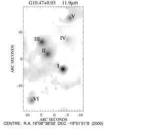
Figure 1: TIMMI2 image at 11.9 $\mu$m with source labeling. Only the positive beams are shown in the figure. The wavelet filtering algorithm of Pantin & Starck (1996) has been applied to enhance the image quality. Source VII lies outside the figure. At about 35″ from the HMC in G10.47, source VII coincides with a UCH ii region in the star-forming region G10.46+0.03 (see Sect. 4.1).

2.2 TIMMI2 imaging

Further mid-infrared observations were performed with the Thermal Infrared Multimode Instrument TIMMI2 (Reimann et al. 2000) mounted on the ESO 3.6m telescope. TIMMI2 can operate like a spectrograph and imager in the M(5 $\mu$m), N(10 $\mu$m) and Q(20 $\mu$m) atmospheric bandpasses. The detector is a 320$\times$240 Si:As High-Background Impurity Band Conduction array with a pixel scale of 0$\aas@@fstack{\prime\prime}$2 in the N and Q imaging modes.

The observations took place in two periods: In May 2001 we imaged the region at 9.8 ($\Delta\lambda$ = 0.9 $\mu$m), 11.9 ($\Delta\lambda$ = 1.2 $\mu$m), 12.9 ($\Delta\lambda$ = 1.2 $\mu$m) and 20.0 $\mu$m ($\Delta\lambda$ = 0.8 $\mu$m) with total integration times of 7, 22, 9, and 14 minutes, respectively; In March 2003 we obtained deeper images in the 11.9, 12.9 and [NeII] ($\lambda$ = 12.8 $\mu$m, $\Delta\lambda$ = 0.2 $\mu$m) filters for a total on-source time of 36, 36, and 30 minutes. During the first run, chop (north-south) and nod (east-west) throws of 10 ″ have been used. In order to enlarge the field of view and thus improve our astrometry (see Sect. 3), we applied a larger chop/nod throw of 20″ during the observations of March 2003.

The standard stars HD 169916 and HD 81797 have been used to flux calibrate the data set from May 2001: HD 169916 at the 11.9 and 12.9 $\mu$m wavelengths, while HD 81797 for the 9.8 $\mu$m and Q band filters. During the second run, we observed the flux calibrator stars HD 123139 at 11.9 $\mu$m and HD 133774 at 12.9 $\mu$m and in the [NeII] filter immediately before and after our target. The corresponding flux densities of all the standards are taken from Cohen et al. (1999). The data reduction was performed as described in Sect. 2.1. The 11.9 $\mu$m image obtained from the reduction of the March 2003 dataset is shown in Fig. 1.

2.3 TIMMI2 spectroscopy

N-band spectroscopy of sources II and III (see Fig. 1) was obtained with TIMMI2 on 31 May 2003. A slit width of 1.2″ was applied yielding to a resolving power of $\sim$170 at 10 $\mu$m. We used the standard chopping/nodding technique along the slit with a throw of 10″. The on-source integration time amounted to 43 minutes for object II and 32 minutes for object III. Both sources were observed at an airmass of $\sim$1.02 during almost photometric conditions. The standard star HD178524 was observed at the same airmass as the targets.

The data reduction was performed using the IDL pipeline kindly provided by R. Siebenmorgen (Siebenmorgen et al. 2004). Smaller modifications were made to speed up the pipeline and improve its robustness. The flux calibration of the spectra was tied to the results of our 12.9 $\mu$m measurements with TIMMI2.

Table 1: Sensitivities (1 $\sigma$) and angular resolutions.

$$\begin{array}[]{p{0.2\linewidth}p{0.1\linewidth}p{0.1\linewidth}p{0.1\linewidth}l}\hline\cr\vskip 3.0pt plus 1.0pt minus 1.0pt\cr Camera&$\lambda$&1\leavevmode\nobreak\ $\sigma$&Resolution${}^{a}$\\ &[\hbox{$\mu$m}]&[mJy/beam]&[\arcsec]\\ \vskip 3.0pt plus 1.0pt minus 1.0pt\cr\hline\cr\vskip 3.0pt plus 1.0pt minus 1.0pt\cr&8.8&21&0.7\\ SpectroCam-10&11.7&9&0.6\\ &17.9&1584&0.9\\ \vskip 3.0pt plus 1.0pt minus 1.0pt\cr\hline\cr\vskip 3.0pt plus 1.0pt minus 1.0pt\cr&9.8&35&1.0\\ TIMMI2(May\leavevmode\nobreak\ 2001)&11.9&8&0.8\\ &12.9&9&0.9\\ &20.0&420&1.4\\ \vskip 3.0pt plus 1.0pt minus 1.0pt\cr\hline\cr\vskip 3.0pt plus 1.0pt minus 1.0pt\cr&11.9&6&0.8\\ TIMMI2(March\leavevmode\nobreak\ 2003)&12.9&4&0.9\\ &[NeII]&11&0.9\\ \vskip 3.0pt plus 1.0pt minus 1.0pt\cr\hline\cr\vskip 3.0pt plus 1.0pt minus 1.0pt\cr ISAAC&2.16&0.017&0.6\\ \hline\cr\end{array}$$

• The angular resolution is given as the FWHM of the observed standard stars for wavelengths smaller than 11 $\mu$m. For longer wavelengths the images are diffraction limited and the angular resolution is the first zero of the Airy ring.

2.4 ISAAC Ks-band imaging

We obtained deep Ks-band images using the ISAAC detector mounted on the Antu unit (UT1) of ESO’s Very Large Telescope at Cerro Paranal, Chile. The observations took place on 20 July 2002 in visitor mode in the ESO-programme 69.C-0189(A). The goal of the observations was to establish a reliable astrometric reference frame to align the MIR detections. Therefore only images at the Ks-band were taken. Due to instrumental problems the long wavelength arm (ALADDIN Array) was used. To avoid the saturation of the bright stars, the shortest possible integration time (0.34s) was applied with a five times repetition at each of the 20 positions. The resulting total observational time was approximately 34 seconds. The field of view was $2.5^{\prime}\times 2.5^{\prime}$. The observations were conducted at an airmass of 1.3 and a (visual) seeing of 0$\aas@@fstack{\prime\prime}$75.

We applied the standard near-infrared (NIR) reduction method to the obtained data as follows: flat fields, bad pixel masking and ’moving sky’ subtraction. The photometry of the resulting image has been carried out by placing an aperture with a radius equal to 2.25″ on the individual sources. The flux calibration was performed using the standard star 9149 from Persson et al. (1998) which was observed at the beginning of the night. We checked the resulting photometry on 10 bright stars also present in the 2MASS database. The estimated error on the photometry is 0.1 magnitude.

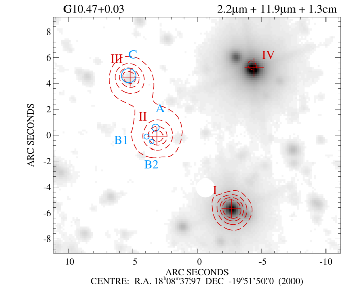
Figure 2: TIMMI2 image at 11.9 $\mu$m (dashed red contour in the electronic version) superimposed on the ISAAC image (grey scale) at 2.16 $\mu$m. Red contour levels go from 6.25 to 25 mJy/${\squareforqed\,\arcsec}$ with steps of 6.25 mJy/${\squareforqed\,\arcsec}$ (source labeling as in Fig. 1). The peak positions of the four MIR sources are marked by red crosses. The blue empty circles correspond to the four UCH ii regions, namely A, B1, B2, and C, observed by CHWC98 in the 1.3 cm continuum. The diameter of the circles coincides with the full width at half power (FWHP$\equiv$FWHM) of the radio emission. The millimeter emission from the HMC peaks at the location of the UCH ii regions B1 and B2 (Olmi et al. 1996a; Gibb et al. 2002). With a white circular aperture we mask source VII which enters in the field because of the adopted chopping/nodding pattern and subsequent image reconstruction procedure. As explained in Sect. 4.1, source VII coincides with the UCH ii region G10.46+0.03A and is located at about 27″ (S-W) from source I.

3 Astrometry

An accurate astrometry is essential to understand the relationship between the MIR emission, the HMC and the UCH ii regions. Interferometric radio continuum maps have good absolute astrometry, usually at the subarcsecond level. However, since the connection between the radio and the MIR emission is not yet clarified, the MIR astrometry should be determined independently from radio measurements.

The detection of up to seven MIR sources in our 11.9 $\mu$m image of March 2003 allows us, for the first time, to establish an independent and accurate astrometric reference frame for the HMC and UCH ii regions. Two different approaches have been tested: One approach (Method A) is based on the 2MASS Second Release Point Source Catalogue (PSC), the other approach (Method B) is based on the USNO2 catalogue combined with our Ks-band image. Both approaches provide a consistent astrometry and are briefly described below.

3.1 Method A

Three presumably stellar MIR sources, namely I, IV, and V (see Fig. 1), have near-infrared counterparts in the 2MASS PSC and were used to derive the astrometry of our MIR images. The standard deviation of the difference between the 2MASS coordinates and the location of the three MIR sources is only 0$\aas@@fstack{\prime\prime}$12. We compared the 2MASS and USNO2 positions of 24 stars within $2^{\prime}$ from our target to estimate the local positional accuracy of the 2MASS catalogue. The standard deviation of the position differences is 0$\aas@@fstack{\prime\prime}$34. Combining the 2MASS-MIR and USNO2-2MASS errors, we estimate an accuracy of 0$\aas@@fstack{\prime\prime}$4 for our 11.9$\mu$m image.

3.2 Method B

In this method, the near-infrared ISAAC image provides the transition from the USNO2 catalogue to our 11.9$\mu$m image. Within the $2.5^{\prime}$ field of our deep Ks-band image, we identified 16 stars which have optical counterparts. Using the USNO2 coordinates we calibrated the astrometry of the ISAAC image with an accuracy of 0$\aas@@fstack{\prime\prime}$26. To establish the astrometry of the MIR image we use four objects detected both at near- and mid-infrared wavelengths (sources I, IV, V, and VI in Fig. 1). The standard deviation of the differences between the NIR and the MIR coordinates is only 0$\aas@@fstack{\prime\prime}$13. Thus, the astrometry of our MIR image is accurate within 0$\aas@@fstack{\prime\prime}$3. The central $22^{\prime\prime}\times 17^{\prime\prime}$ of our Ks-band image together with the superimposition of the 11.9$\mu$m contour and the location of the UCH ii regions is shown in Fig. 2.

Figure 3: Cuts through the MIR emission of the sources II and III obtained on the wavelet-filtered images. The width of the cut is 3 pixels. The intensity is normalized to the peak of the MIR source II. Left: cut along the line connecting the peaks of the two MIR sources. A faint ”bridge” of emission is visible between the peaks at 11.9 $\mu$m. Similar faint emission is also present in the non wavelet-filtered images. Right: cut in the perpendicular direction for source II showing different sizes at different wavelengths.

4 Immediate results

4.1 Imaging

Seven MIR sources can be identified in our more sensitive 11.9$\mu$m image taken during the second TIMMI2 observing run. An overview on the designation is given in Fig. 1. Five of the MIR sources are also detected at 12.9$\mu$m and in the [NeII] filter. Only the sources from I to IV are present in the smaller field of the Spectro-Cam observations (see Table 2). Sources I, IV, V and VI have NIR counterparts and are used to determine the astrometric reference frame of our MIR images as explained in Sec. 3. None of them shows radio emission in the 1.3 cm (CHWC98) and 6 cm (WC89) continuum maps. Source VII is at about 35″ south-west of the HMC in G10.47 and coincides, within our astrometric accuracy, with the UCH ii region G10.46+0.03A.

The most interesting MIR sources are II and III because of their vicinity to a group of UCH ii regions (G10.47A, B1, B2, and C) and to the HMC. They appear marginally extended in the [NeII] and in the 12.9$\mu$m filters and more extended at 11.9$\mu$m. We detect faint emission at this wavelength between the two sources: this ”bridge” might be due to the larger extension of the sources at 11.9$\mu$m. In Fig. 3 we show a cut along the direction connecting the peak positions in two different filters and an additional perpendicular cut for source II.

The UCH ii region C is found to have a mid- and a near-infrared counterpart in our images (see Fig. 2): The NIR, MIR and radio peaks are coincident within our astrometric accuracy. The 2.16 $\mu$m emission is marginally extended and amounts to 0.22 mJy. Assuming a Gaussian profile both for the source (FWHM = 0$\aas@@fstack{\prime\prime}$67) and for the beam (FWHM = 0$\aas@@fstack{\prime\prime}$56), we calculate a deconvolved FWHM at 2.16 $\mu$m of 0$\aas@@fstack{\prime\prime}$4 for source III. The MIR emission is more extended, the deconvolved source size amounts to 1.8″ at 11.9 $\mu$m. For comparison, the 1.3 cm radio continuum emission is 0$\aas@@fstack{\prime\prime}$88 (CHWC98) with an extended spherical halo of 3″ detected in the lower resolution 6 cm radio map of Garay et al. (1993).

We do not detect NIR emission in the direction of the HMC and the three UCH ii regions A, B1 and B2. Our NIR upper limit of 0.05 mJy/beam (3 $\sigma$ sensitivity) translates into a Ks limiting magnitude of 17.8 mag. Radio measurements predict at least an O9.5 type star as ionizing source of the UCH ii region A and B0 type stars in the case of the UCH ii regions B1 and B2. The apparent Ks magnitude for an O9.5/B0 star located at the distance of G10.47 is 10.3/10.4 mag (intrinsic infrared colors from Tokunaga 2000 and absolute visual magnitude from Vacca et al. 1996). Considering the non-detection at NIR wavelengths and the apparent magnitudes calculated above, we find that the extinction towards the HMC and UCH ii regions is at least 7.4 magnitudes at 2 $\mu$m. This value translates into a column density of 10²³ cm^-2 when we adopt the extinction curve and the conversion factor to N_H from Weingartner & Draine (2001). For comparison, column density estimates obtained from molecular lines are at least two times larger (Olmi et al. 1996a, CHWC98, Hofner et al. 2000).

The measured flux densities and peak positions of the seven MIR sources are provided in Table 2. Note that the flux densities related to the [NeII] filter include a contribution from the continuum as well as from the [NeII] line emission. The given total fluxes correspond to the fluxes within a synthetic aperture of 4 ″. The errors of each flux measurement are estimated to be of 15% for the sources from I to IV, and 20% for sources V, VI and VII. We report no detection in the 8.8, 9.8, 17.9 and 20 $\mu$m filters. In these cases the upper limits for the flux densities can be deduced from the sensitivities given in Table 1.

We note that the IRAS source 18056-1952, which was considered to be the infrared counterpart of the complex massive star-forming region G10.47 (e.g. WC89, Hatchell et al. 2000), has a 12 $\mu$m flux of 7.93 Jy, more than 10 times larger than the total flux we measure from the seven MIR sources. This, together with the fact that none of our MIR sources is located inside the IRAS pointing accuracy ellipse excludes that the IRAS source is related to G10.47. For completeness, we mention that the Midcourse Space Experiment (MSX) detected a bright unresolved source at 21.3$\mu$m whose peak position is at about 3.7″ south-east from our MIR source II. The MSX position accuracy is about 2″ both in right ascension and declination and the flux measured in the MSX beam amounts to 22$\pm$1 Jy. The large 18″ MSX beam includes all our MIR sources but source VII. However, considering the steep rise in the spectral energy distribution (SED) of HMCs (Osorio et al. 1999) we expect that the HMC in G10.47 contributes most of the flux at 21.3$\mu$m.

Table 2: Measured flux densities and peak positions of the MIR sources (source labeling as in Fig. 1). Source VII belongs to the star-forming region G10.46+0.03, see Sect. 4.1 for more details.

$$\begin{array}[]{p{0.08\linewidth}p{0.11\linewidth}p{0.11\linewidth}p{0.1\linewidth}p{0.1\linewidth}p{0.1\linewidth}p{0.1\linewidth}l}\hline\cr\vskip 3.0pt plus 1.0pt minus 1.0pt\cr Source&\lx@intercol\hfil\rm{Peak\leavevmode\nobreak\ Position}\hfil\lx@intercol&F${}_{{\rm 11.7}}$${}^{\mathrm{a}}$&F${}_{{\rm 11.9}}$${}^{\mathrm{b}}$&F${}_{{\rm 12.9}}$${}^{\mathrm{b}}$&F${}_{{\rm[NeII]}}$${}^{\mathrm{b}}$\\ \vskip 3.0pt plus 1.0pt minus 1.0pt\cr ID&$\alpha(2000)$&$\delta(2000)$&&&&\\ &[h m s]&[${}^{\circ}$ ${}^{\prime}$ ${}^{\prime\prime}$]&[mJy]&[mJy]&[mJy]&[mJy]\\ \vskip 3.0pt plus 1.0pt minus 1.0pt\cr\hline\cr\vskip 3.0pt plus 1.0pt minus 1.0pt\cr I&18 08 37.78&-19 51 55.7&101&170&154&220\\ II&18 08 38.19&-19 51 50.0&140&136&457&943\\ III&18 08 38.34&-19 51 45.6&131&137&236&703\\ IV&18 08 37.66&-19 51 44.8&23&30&$<$12&$<$33\\ V&18 08 37.59&-19 51 36.6&---&107&$<$12&$<$33\\ VI&18 08 38.61&-19 52 07.3&---&94&201&424\\ VII&18 08 36.47&-19 52 14.9&---&89&160&309\\ \hline\cr\end{array}$$

• The flux densities are computed in the broad-band 11.7, 11.9 and 12.9 $\mu$m filters and in the narrow-band [NeII] filter. The estimated flux uncertainty is 15% for sources from I to IV and 20% for sources V, VI and VII

• Symbol ”—” indicates that sources V, VI and VII are outside the SpectroCam field

• Flux densities from the second TIMMI2 run, upper limits represent 3 $\sigma$ sensitivities.

4.2 MIR spectroscopy

The calibrated N-band spectra of sources II and III are shown in Fig. 4. A reliable removal of the atmospheric lines is reached in the wavelength range 8–13 $\mu$m. The error plotted on each point represents the flux scatter due to photon noise, additional noise may come from the improper subtraction of telluric lines.

The spectrum of object II is clearly dominated by the silicate absorption feature. The [NeII] emission line at 12.81 $\mu$m is detected with a line-to-continuum ratio of about 1.5. In contrast, the spectrum of source III shows strong [NeII] line emission and weak silicate absorption. None of the other MIR fine-structure lines, like [ArIII] at 8.99 $\mu$m and [SIV] at 10.51 $\mu$m, can be identified in the spectra. Following Okamoto et al. (2001) and Okamoto et al. (2003), we estimate upper limits for the ionizing stars from the flux ratio of the non-detected [ArIII] and [SIV] and the [NeII] emission line. Upper limit fluxes for the [ArIII] and [SIV] lines are obtained by integrating the de-extincted spectra (see Sec. 5.1 for the procedure) in a 0.06 $\mu$m interval centered on 8.99 $\mu$m and 10.51 $\mu$m, respectively. For source II we estimate an O7 type star, while for source III we obtain an O9 type star as upper limits. We note that this method is model-dependent: The observed flux ratios are compared to CoStar calculations by Stasinska & Schaerer (1997). In the next section, we apply a different method which only depends on the observed [NeII] flux to estimate the Lyman continuum flux and thus to determine the spectral types of the ionizing sources.

Figure 4: N-band spectroscopy of source II and III. The fine-structure emission lines from metal ions are marked with solid lines (detection) and dashed lines (non detection).

5 Discussion on the individual sources

In the following, we discuss the MIR sources with special attention on sources II and III, which are close to the UCH ii regions and the HMC in G10.47.

5.1 Source III and the ultra-compact H ii region C

Source III is the mid-infrared counterpart of the UCH ii region C (WC89). Further radio measurements (Garay et al. 1993 and CHWC98) show that a B0 or earlier type star is responsible for its ionization. We also detect its NIR counterpart in our Ks-band image (see Sect. 4.1). This slightly elongated counterpart has a total flux of 0.22 mJy at 2.16 $\mu$m, which corresponds to a Ks magnitude of 16.2. The apparent K magnitude for a B0 star at the distance of G10.47 is 10.4 mag (intrinsic infrared colours from Tokunaga 2000 and absolute visual magnitude from Vacca et al. 1996). Thus, we calculate an extinction $A_{2.2}$ of 5.8 mag at 2.2 $\mu$m. However, this value only represents a lower limit: part of the observed emission at this wavelength may come from scattered light in a non-spherical configuration and from warm dust surrounding the UCH ii region. The presence of warm dust around the UCH ii region is evident at longer wavelengths where the source appears more extended ($\sim$ 1.8″ at 11.9 $\mu$m after deconvolution with the diffraction-limited beam) and has a flux more than 500 times larger than the extincted black body emission from the star.

To obtain a more accurate value for the extinction and to estimate the spectral type of the ionizing source independently from the radio measurements, we use our MIR spectrum. We assume a simple model in which the MIR flux from warm dust is described by a black body of temperature T_d as optically thick emission and is extinguished by a screen of cold dust in the foreground. For sake of simplicity we do not distinguish between the cold dust in the interstellar medium and that in the molecular cloud. With these assumptions, the observed flux density can be expressed as:

$$F_{\nu}=\Theta^{2}\,B_{\nu}(T_{\rm{d}})\,exp(-\tau_{\nu})$$ (1)

with $\Theta$ being the angular diameter of the source of warm dust, $T_{\rm{d}}$ the temperature of the emitting dust and $\tau_{\nu}$ the optical depth of the cold dust layer. The optical depth $\tau_{\nu}$ is proportional to the line-of-sight column density $N_{\rm{(H+H_{2})}}$ through the dust extinction cross section per hydrogen nucleon C${}_{\rm ext}(\nu)$. These latter values are taken from Draine (2003), who recently revised the grain size distributions and dielectric functions used to produce the previous synthetic extinction curves (Weingartner & Draine 2001). We consider two extinction laws for the local Milky Way, one typical for diffuse regions ($R_{\rm{V}}$=3.1) and one for sightlines intersecting clouds with larger extinction ($R_{\rm{V}}$=5.5). The continuum of the observed spectrum (7.9–12.75 $\mu$m and 12.9–13.1 $\mu$m) is fitted by using equation 1 with $b$, $T_{\rm{d}}$, and $N_{\rm{(H+H_{2})}}$ as free parameters. A robust least-square minimization using the Levenberg-Marquardt method is performed to derive the best fit parameters and their 1$\sigma$ uncertainties which are computed from the covariance matrix. The two extinction laws provide the same results within the errors, the best-fit parameters are summarized in Table 3. From the estimated line-of-sight column density we derive an extinction of 4 magnitude at 9.8 $\mu$m. This value translates into $A_{2.2}$ = 6.7 magnitude, about 1 magnitude greater than the extinction estimated from the apparent Ks magnitude and the expected flux of a B0 star. This means that about half of the measured Ks emission is photospheric flux from the ionizing star, the remaining originates from dust re-emission.

To estimate the spectral type of the ionizing source we will use the de-extincted flux in the [NeII] line ($I_{12.8}^{0}$) and a formula which links this quantity to the number of ionizing photons per second ($Q_{0}$). The determination of the de-extincted flux in the [NeII] line is done as follows: First, we subtract the fitted continuum from the spectrum, then we de-extinct the [NeII] flux density by the measured $\tau_{\nu}$, finally we compute the integral in the [NeII] line between 12.75 and 12.9 $\mu$m and the error on the integrated flux as the sum of the errors at each sampled wavelength. The formula connecting $I_{12.8}^{0}$ and $Q_{0}$ is derived assuming a spherically symmetric, optically thin (CHWC98), homogeneous, ionization-bounded H ii region. The intrinsic flux of an emission line as a function of the radio continuum is given by equation (8) of Martín-Hernández et al. (2003). Equation (5) from Martín-Hernández et al. (2003) provides the number of Lyman continuum photons as a function of the radio continuum. The ratio of these two equations allows to express $Q_{0}$ as a function of the de-extincted flux in the [NeII] line:

$$Q_{0}=2.566\times 10^{34}\,T_{\rm e}^{-0.8}\,D^{2}\,\frac{I_{12.8}^{0}}{(Ne^{+}/H^{+})\,\epsilon_{12.8}}\,\,[s^{-1}]$$ (2)

In equation 2, $T_{\rm e}$ is the electron temperature in K, $D$ the source distance in kpc, $I_{12.8}^{0}$ the de-extincted flux density of the [NeII] line in erg s^-1 cm^-2 and $\epsilon_{12.8}$ the line emissivity in erg s^-1 cm³. The term $(Ne^{+}/H^{+})$ is the abundance of ionized neon over ionized hydrogen. The absence of [ArIII] and [SIV] lines in our spectrum shows that the nebula is of low-excitation and therefore we can further assume $(Ne^{+}/H^{+})\sim(Ne/H)$. The abundance of Ne relative to H is calculated for the specific galactic distance of G10.47 from the equation given in Martín-Hernández et al. (2003). For a galactocentric distance of 2.5 kpc we compute a value of $2.2\times 10^{-4}$ for $(Ne/H)$, which is about two times the solar abundance (Grevesse & Sauval 1998). The calculation of the line emissivity $\epsilon_{12.8}$ is done following the formulation of Osterbrock (1974) (equations 3.25, 4.12 and 5.29) and assuming atomic data from Saraph & Tully (1994). We obtain a value of 4.6$\times$10^-23 erg s^-1 cm³ for a $T_{\rm e}$ of 10000 K and an electron density of $4.2\times 10^{4}$ cm^-3 as given by CHWC98. The resulting number of Lyman continuum photons with the uncertainty estimated from the error in the [NeII] flux and from the two extinction curves is provided in Table 3. Our value is about three times larger than that estimated by CHWC98 from the measured radio continuum emission.

Determining the spectral type of the ionizing star from the $Q_{0}$ parameter requires a careful consideration of the recent results from O-star atmosphere models. Martins et al. (2002) demonstrated that a proper treatment of non-LTE line blanketed atmospheres shifts the effective temperature scale of O stars towards lower values for a given spectral type in comparison to simpler LTE approaches (Vacca et al. 1996). Recently, Mokiem et al. (2004) compared the output of different O-star models and concluded that the relation between $Q_{0}$ and $T_{\rm eff}$ is largely model independent. Based on these two results, we adopt the following procedure to derive the spectral type of the ionizing source: First we choose the $T_{\rm eff}$ that matches our computed Log($Q_{0}$) from Table 3 of Schaerer & de Koter (1997) and then we link the temperature to the spectral type using Fig. 1 from Martins et al. (2002). In the case of source III the estimated number of Lyman continuum photons is slightly lower than the lowest value given in Table 3 of Schaerer & de Koter (1997) which implies an effective temperature below 32000 K. These temperatures translate into a B0 spectral type which is in good agreement with the spectral type estimated by CHWC98 based on the old temperature scale of Panagia (1973). In order to check the reliability of our approach, we also compute the radio flux at 1.3 cm that we expect from equation (8) of Martín-Hernández et al. (2003) and we compare it with the 1.3 cm flux obtained from CHWC98. Assuming the same values as above and the de-extincted flux in the [NeII] line provided in Table 3, we calculate a flux of 154$\pm$10 mJy at 1.3 cm. This value is about five times larger than that given in Table 3 by CHWC98. One reason for this discrepancy might be that some flux is lost in the high resolution VLA configuration. To prove this we compared two measurements at 6 cm by WC98 and Garay et al. (1993) obtained with two different angular resolutions (about 0$\aas@@fstack{\prime\prime}$5 and 4.7″ respectively). This comparison shows that the flux from Garay et al. (1993) is about three times larger than that from WC98 at 6 cm, thus proving that the more extended VLA configuration indeed overlooked some of the flux from large-scale structures. If a similar flux ratio would have been lost in the 0$\aas@@fstack{\prime\prime}$4 resolution map of CHWC98 at 1.3 cm, the radio flux estimated from our [NeII] line would be only 1.7 time the expected radio flux at 1.3 cm. Given the simple approach we used here, this match is a reasonable good agreement.

Our infrared images and spectrum show that the B0 star ionizing the UCH ii region C is surrounded by dust which is optically thick at these wavelengths. Thus, we cannot use the infrared fluxes to estimate the amount of dust surrounding the UCH ii region. However, we can derive upper limits for the dust mass from the BIMA non-detection at 1.4 mm (Gibb et al. 2002). In the natural weighted BIMA map the 1 $\sigma$ detection limit is 20mJy/beam for a beam of 1.98 ″$\times$1.27 ″ (Wyrowski priv. comm.). We assume optically thin emission at 1.4 mm, two values for the dust temperature (30 and 50 K) and the mass absorption coefficient of the dust from Ossenkopf & Henning (1994) for a gas density of 10⁵ cm^-3. A dust mass between 0.2–0.4 M_☉ is derived. This value translates into a total mass of 20–40 M_☉ if a gas/dust mass ratio of 100 is adopted. The corresponding upper limit column densities are 1.9–3.5$\times$10²³ cm^-2 for the molecular hydrogen (see eq. 2 and 3 of Henning et al. 2000), well in agreement with the value we estimate by fitting the MIR continuum of our N-band spectrum (Table 3).

Table 3: Best fit parameters to the N-band spectra and estimated spectral types for the ionizing sources

$$\begin{array}[]{p{0.08\linewidth}p{0.16\linewidth}p{0.1\linewidth}p{0.1\linewidth}l}\hline\cr\vskip 3.0pt plus 1.0pt minus 1.0pt\cr Parameter${}^{a}$&Unit&Source II&Source III\\ \vskip 3.0pt plus 1.0pt minus 1.0pt\cr\hline\cr\vskip 3.0pt plus 1.0pt minus 1.0pt\cr$T_{\rm d}$&(K)&271$\pm$19&324$\pm$47\\ $N_{\rm(H+H_{2})}$&($\times 10^{22}$\,cm${}^{-2}$)&23$\pm$2&8$\pm$1\\ $\Theta$&(mas)&29$\pm$16&5$\pm$4\\ $\tau_{9.8}$&&9&4\\ $I_{12.8}$&($\times 10^{-13}$\,erg\,s${}^{-1}$\,cm${}^{-2}$)&4.9$\pm$0.8&19$\pm$1\\ $I_{12.8}^{0}$&($\times 10^{-12}$\,erg\,s${}^{-1}$\,cm${}^{-2}$)&9$\pm$2&7.0$\pm$0.4\\ log(Q${}_{\rm 0}$)&(s${}^{-1}$)&47.7$\pm$0.1&47.5$\pm$0.1\\ $T_{\rm eff}$&(K)&32060&$<$32060\\ SpTy&&O9.7&B0\\ \hline\cr\end{array}$$

• $T_{\rm eff}$ is determined from Table 3 of Schaerer & de Koter (1997), while the spectral type (SpTy) from Fig. 1 of Martins et al. (2002).

5.2 Source II and its relation with the hot molecular core

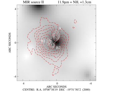
Figure 5: Image of the MIR source II at 11.9 $\mu$m with contours of the 1.3 cm radio continuum (solid white lines) and of NH₃(4,4) line emission (red dashed lines in the electronic version) from CHWC98. White contour levels are spaced by 7 mJy/beam starting from 5 to 33 mJy/beam, red-dashed contours are spaced by 4 mJy/beam from 3 to 27 mJy/beam.

Source II is the most exciting among our MIR detections. Three UCH ii regions and a HMC have been identified by CHWC98 in this region. CHWC98 suggest a picture in which the three massive stars, at the stage of UCH ii regions, are embedded in the dense molecular core traced by ammonia emission. Since the UCH ii regions B1 and B2 are more compact than A and show more absorption in the NH₃(4,4) transition, CHWC98 propose that A is lying closer to the surface of the HMC traced in ammonia, i.e in a less dense region. The fact that the three UCH ii regions are tracing embedded stars is supported by the compactness of their radio emission: The two VLA 6 cm maps from WC89 and Garay et al. (1993) at different resolution provide the same total flux for the three UCH ii regions. To show the complexity of this region we superimpose the radio, ammonia and mid-infrared emission in Fig. 5.

Up to now, only few cases are known in which MIR emission is detected from the close vicinity of HMCs (De Buizer et al. 2002, 2003). Proving that such emission arises from the HMC itself would support the idea of internally heated cores. In Sect. 3 we demonstrated that our astrometry is accurate to 0$\aas@@fstack{\prime\prime}$3 based on stars with counterparts at different wavelengths. This high accuracy allows to explore the relation between the UCH ii phenomena, the HMC and the MIR emission. Here, the main question is whether the MIR emission is indicating the presence of a protostar, or of a young massive star prior to the UCH ii phase, or arises from dust surrounding the UCH ii regions. To answer this question we use both the mid-infrared images and the spectroscopic data.

Before investigating the three scenarios, we briefly summarize the main observational results:
I) Based on our astrometry, none of the UCH ii regions coincides with the mid-infrared peak of source II: this peak is located south of the UCH ii region A, at about the same distance ($\sim$0$\aas@@fstack{\prime\prime}$6 = 3480 AU) from A and B2. The UCH ii region B1 is further away from source II at about 0$\aas@@fstack{\prime\prime}$8. The MIR emission does not coincide with the center of the HMC, which is believed to be close to the most embedded UCH ii regions B1 and B2.
II) The MIR emission is extended in the NW-SE direction even in the [NeII] filter (deconvolved FWHM of 0$\aas@@fstack{\prime\prime}$9 after the continuum subtraction). The MIR extension is even larger at 11.9$\mu$m, about 1.8″ (see Fig. 3 and Sect. 4.1).
III) The MIR spectrum does not show the forbidden lines of [ArIII] and [SIV] thus implying an O7 upper limit for the spectral type of the ionizing source (see Sect. 4.2).
IV) The combination of PdBI data with IRAM 30-m maps in the CH₃CN(6-5) line led Olmi et al. (1996a) to identify an extended halo around a compact core. The compact core well matches the location and extension of the ammonia HMC (CHWC98). Assuming an abundance of CH₃CN relative to H₂ of $\sim$10^-8 (Hatchell et al. 1998; Olmi et al. 1993) the column densities of Table 3 from Olmi et al. (1996a) translate into H₂ core and halo column densities of $\sim$6$\times$10²⁴ cm^-2 and $\leq$3.6$\times$10²³ cm^-2. The upper value for the halo column density agrees well with the column density we measure towards source II from fitting our MIR spectrum (see Table 3). However, considering the different techniques and angular resolutions of the observations, we cannot determine the exact line-of-sight location of source II in respect to the HMC.
V) The slope of the radio emission as given from the measurements at 6 cm (WC89) and 1.3 cm (CHWC98) is $S_{\nu}\propto\nu^{0.9}$ for the UCH ii region A and $S_{\nu}\propto\nu^{1.4}$ for B. Both slopes are different from that expected in the case of ionization due to a spherical stellar wind ($S_{\nu}\propto\nu^{0.6}$, Panagia & Felli 1975). Also the size of the UCH ii region A increases towards shorter wavelengths, contradicting the wind hypothesis ($R_{\nu}\propto\nu^{-0.7}$, Panagia & Felli 1975).

We now consider the first two scenarios, namely a massive protostar or a massive star embedded in the HMC at a stage prior to the UCH ii phase. In the protostellar phase, accretion provides most of the luminosity and the Lyman continuum emission is expected to be much fainter than for a ZAMS O-B star. This stands in evident contradiction with the observed presence of the [NeII] emission from source II, effectively excluding its massive protostar nature. Furthermore, the detection of [NeII] emission from source II implies a radio continuum emission as large as 265$\pm$59 mJy at 1.3 cm ($I_{12.8}^{0}$ from Table 3 and equation (8) from Martín-Hernández et al. 2003). Such radio continuum is well above the sensitivity of the 1.3 cm map from CHWC98, the non-detection at the location of source II demands a suppressing mechanism. In a stage prior to the UCH ii, accretion could quench the radio free-free emission (Yorke 1986) and constrain the ionized hydrogen into a small dust-evacuated cavity of radius $R_{c}\,\sim\,(L_{*}/4\pi\sigma\,T_{\rm d}^{4})^{1/2}$ (see e.g. Churchwell 2002a). Using the same approach as for source III, we determine a lower-limit spectral type between B0 and O9.5 (see Table 3). For these spectral types, the extent of the ionized region is well traced by the [NeII] line emission. For a luminosity of 10⁵ L_☉ (Vacca et al. 1996) and dust sublimation temperature $T_{\rm d}\sim 1000$ K, we estimate an $R_{c}$ of about 50 AU, which is 0$\aas@@fstack{\prime\prime}$008 at 5.8 kpc distance. Thus, the typical size of an accretion-quenched H ii region would be more than two orders of magnitudes smaller than the observed size in the [NeII] line. Therefore, we conclude that no massive star prior to the UCH ii phase can be responsible for the observed [NeII] emission.

In the third scenario, we assume that the warm dust around one or more of the UCH ii regions A, B1 or B2 is the source of the mid-infrared flux. We will have then to demonstrate that: 1) The young massive star ionizing the UCH ii region can maintain an ionized halo detectable in the mid-infrared and showing [NeII] emission at the location of source II; 2) The shift between radio and mid-infrared emission can be explained by extinction, geometry and/or clumping.

The projected distance between the peak of the mid-infrared source II and the most distant UCH ii region B1 is 0$\aas@@fstack{\prime\prime}$8, 0.02 pc at the distance of G10.47. The spectral types of the stars ionizing the UCH ii regions A, B1 and B2 are estimated to be B0–O9 or earlier from radio measurements (CHWC98). These spectral types agree with our O7 upper limit obtained from the ratio of the non-detected and detected forbidden emission lines . The CoStar ionization models predict that the [NeII] emission can extend up to 0.055 pc from B0–O9 stars and up to 0.083 pc from O9–O8 stars embedded in spherically symmetric ionized regions with uniform electron density (see Fig. 13 of Okamoto et al. 2003, and text therein). Thus, the stars powering the UCH ii regions A, B1 and B2 can indeed provide sufficient ionization to explain the observed [NeII] emission.

To explain the apparent shift of the mid-infrared peak from the radio peaks, we consider the following situation: The UCH ii regions lie in the direction of high line-of-sight extinction and are surrounded by warm dust emitting at mid-infrared wavelengths. The peak of the MIR emission would coincide with the UCH ii regions, but due to the extinction gradient the peak is apparently shifted towards the direction of lower extinction. Thus, the MIR-radio continuum offset is the result of extinction and geometry of the sources. In the following more detailed discussion we shall further distinguish between the UCH ii region A, lying closer to the surface of the ammonia molecular core probably in the halo, and the UCH ii regions B1 and B2 closer to the center of the HMC (CHWC98, Olmi et al. 1996a).

First, we consider the case of the two more embedded UCH ii regions B1 and B2 and investigate if such embedded sources could be detected in our MIR images. CHWC98 estimated B0 spectral types for the stars ionizing the UCH ii regions B1 and B2 similarly to the UCH ii region C. We detected MIR emission from dust around the UCH ii region C (source III) and we can now calculate up to which extinction/column density such emission would be detectable in our most sensitive 12.8 $\mu$m broad-band images (see Table 1). By fitting the MIR spectrum of source III we found an extinction of 4 mag at 9.8 $\mu$m (Table 3) that translates into 1.3 mag at 12.8 $\mu$m assuming the extinction laws from Draine (2003). The measured flux of source III (see Table 2) corresponds to a de-extincted flux of 1 Jy in the 12.8 $\mu$m filter. Already an extinction/column density 5 times larger than that measured towards source III reduces the flux density to only 1.5 mJy, that is below the 1 $\sigma$ sensitivity of our 12.8 $\mu$m images. For comparison, the core averaged column density from Olmi et al. (1996a) is more than 70 times the column density towards source III (see Table 3). Thus, we conclude that no mid-infrared emission from dust surrounding the UCH ii regions B1 and B2, located close to the core center, could have been detected in our MIR exposures. We note, however, that the simple approach applied above neglects the clumpiness of the core. Should the geometry strongly deviate from the homogenous distribution, radiation from the UCH ii regions B1 and B2 might also contribute to the MIR flux.

Proving that the MIR emission comes from dust around the UCH ii region A is beyond the possibility of this dataset. However, three facts support this scenario. First, the column density we measure towards source II is similar to the averaged column density measured by Olmi et al. (1996a) in the halo around the ammonia HMC, where the UCH ii A is probably located. Second, the radio emission estimated from the [NeII] line strength (see above) closely resembles the observed 1.3 cm flux from the UCH ii region A (within a factor of two), while showing a larger difference from the 1.3 cm flux of B1 and B2. Third, we find a marginal shift in the peak location of source II between the broad-band 11.9$\mu$m filter and the [NeII] narrow-band filter: The [NeII] peak of source II is 0$\aas@@fstack{\prime\prime}$1 N-E of the 11.9$\mu$m peak emission, i.e. the peak is closer to the UCH ii region A.

5.3 The other mid-infrared sources

In the large field of view of the images from the second TIMMI2 run we detected seven MIR objects. The sources II and III belong to the massive star forming region G10.47 and have been described in the previous two Sections. Source VII is the MIR source located at the largest distance from the HMC in G10.47 and is found to coincide with the UCH ii region G10.46+0.03A within our astrometric accuracy. To investigate the nature of the other four MIR sources, we retrieve their NIR magnitudes from the 2MASS PSC and we plot their colours in a NIR colour-colour diagram (for the use of the colour-colour diagram we refer to Lada & Adams 1992). The colors of main sequence, giant and supergiant stars are taken from Tokunaga (2000).

Source I lies on the right side of the main-sequence stripe, thus indicating NIR excess. This excess is thought to originate from hot circumstellar dust. The presence of dust around source I is confirmed by our MIR images: Source I appears slightly extended in the broad band filters (deconvolved FWHMs of $\sim$ 1″ at 11.7 and 11.9 $\mu$m and 0$\aas@@fstack{\prime\prime}$5 at 12.9 $\mu$m) and has an SED slowly increasing towards longer wavelengths (see Table 2). The continuum-subtracted [NeII] images show no emission. Although the further discussion of this object is out of scope of the current paper, we note that the lack of the [NeII] and free-free radio emission proves that this star is not a massive (earlier than B0 spectral type) young stellar object.

Sources IV and V lie within the region of reddened main-sequence stars. To determine their spectral types and luminosity classes we adopt the following method: I) By shifting these sources back on the colour-colour diagram – along the reddening vector – we find the possible spectral type/luminosity class combinations. II) From the difference between the old and new location in the colour-colour diagram we estimate the extinction. The distance is given by the comparison of the apparent and the absolute magnitudes taking the derived extinction into account. III) As the last test, we compare the 11.9 $\mu$m flux of this hypothetical star (at the given distance and extinction) to our measured MIR flux. With this approach we find that sources IV and V are strongly reddened (A${}_{\rm V}>20$ mag). Should they be dwarf stars, they would necessarily lie within a distance of 80 pc to fit the apparent brightness we observed. However, comparing the A${}_{\rm V}>20$ mag to the mean extinction value of 1.9 V-mag/kpc of the Milky Way disk (Allen 1973), we can exclude that these sources are reddened main sequence stars. For MIR IV the most probable nature is that of a G0-G3 supergiant at a distance of about 5 kpc, although the measured MIR flux at 11.9 $\mu$m is slightly lower than that estimated from a black body approximation ($\sim$44 mJy) of the photosphere. Similarly, source V is consistent with a supergiant of spectral type B6 at a distance of 2.5 kpc and an extinction of 30 mag in V.

6 Summary

We observed the massive star-forming region G10.47 at infrared wavelengths in order to study in detail the relationship between the HMC and the UCH ii regions. An astrometric accuracy at the subarcsecond level and additional spectroscopy of the two most interesting MIR sources allow us to draw the following main conclusions:

1. We detect extended MIR emission (source II) towards the HMC and the three UCH ii regions. However, the MIR emission does not coincide with the HMC position nor with the position of any of the UCH ii regions. The most plausible scenario is the one in which the MIR emission of source II originates from dust heated by the UCH ii region A, one of the three embedded UCH ii regions in the HMC. The shift in the peak emission between the ionizing star and the MIR emission is interpreted as due to geometrical effect and changes in the extinction. This scenario is supported by the marginal shift of the peak positions found at 11.9 $\mu$m and in the [NeII] filter.

2. The UCH ii region C, which is located outside the HMC, is found to have a mid- and a near-infrared counterpart. From our MIR spectroscopy we derive a B0 spectral type for the star ionizing the UCH ii region C. This spectral type agrees well with that found from radio free-free emission (CHWC98). The size of the radio free-free emission together with the relatively low column density towards the source suggest that the UCH ii region C could have evolved rapidly because of a relatively low density environment.

3. The mid-infrared source VII is coincident with a UCH ii region in the star forming region G10.46+0.03.

4. The mid-infrared source I shows infrared excess thus indicating the presence of surrounding warm dust. The absence of [NeII] and free-free radio emission proves that the star has a spectral type not earlier than B0.

5. Combining the 2MASS fluxes with our MIR observations we find that the mid-infrared sources IV and V are possibly supergiant stars in the foreground of the massive star-forming region G10.47.