Power spectrum estimation from high-resolution maps by Gibbs sampling
Abstract
We revisit a recently introduced power spectrum estimation technique based on Gibbs sampling, with the goal of applying it to the high-resolution WMAP data. In order to facilitate this analysis, a number of sophistications have to be introduced, each of which is discussed in detail. We have implemented two independent versions of the algorithm to cross-check the computer codes, and to verify that a particular solution to any given problem does not affect the scientific results. We then apply these programs to simulated data with known properties at intermediate () and high () resolutions, to study effects such as incomplete sky coverage and white vs. correlated noise. From these simulations we also establish the Markov chain correlation length as a function of signal-to-noise ratio, and give a few comments on the properties of the correlation matrices involved. Parallelization issues are also discussed, with emphasis on real-world limitations imposed by current super-computer facilities. The scientific results from the analysis of the first-year WMAP data are presented in a companion letter.
Subject headings:
cosmic microwave background — cosmology: observations — methods: numerical1. Introduction
The subject of cosmic microwave background (CMB) power spectrum estimation has been a very active research field for many years now, and the combined effort from the scientific community has resulted in a number of qualitatively different methods. Broadly, one may classify these methods into three groups, namely maximum likelihood methods (Górski, 1994, 1996; Tegmark, 1997; Bond, Jaffe & Knox, 1998; Oh et al., 1999; Doré, Knox & Peel, 2001), pseudo- methods (Wandelt, Hivon & Górski, ; Hivon et al., 2002; Hansen, Górski & Hivon, 2002; Hansen & Górski, 2003), and specialized methods (van Leeuwen et al., 2002; Challinor et al., 2002; Wandelt & Hansen, 2003). In general the maximum likelihood methods are more accurate than the (often Monte Carlo based) pseudo- methods, but they are usually so at a prohibitive computational cost. And even these methods can only return very approximate summaries of the error bars, since exploring the likelihood away from the peak is practically impossible. Further, the specialized methods are usually only applicable following rather restrictive assumptions. For general experiments we have up to now been left with the rather uncomfortable choice between the optimal but prohibitively expensive, and the feasible but approximate.
In this context, a method based on Monte Carlo Markov Chains and Gibbs sampling was very recently developed by Jewell, Levin & Anderson (2004) and Wandelt, Larson & Lakshminarayanan (2004) which may change this picture. The fundamental idea behind this method is to solve the power spectrum estimation problem by establishing its posterior probability distribution through sampling, rather than by direct solution of the corresponding optimization problem. In its most general form, the scaling of this Monte Carlo method equals that of the map making process, which is to be compared to the typical scaling for traditional maximum likelihood estimators (Borrill, 1999), being the number of pixels in the map. Further, for an experiment with spherically symmetric beams and uncorrelated noise, one may work directly with maps instead of time-ordered data, in which case the scaling reduces to that of a spherical harmonics transform, namely , using the HEALPix111http://www.eso.org/science/healpix/ pixelization.
Until now, the only application of this method to cosmological data was the analysis of the low-resolution COBE-DMR data, presented by Wandelt et al. (2004). In the following we demonstrate the practicality of this method for current and future experiments, as we for the first time apply it to a large data set, namely the Wilkinson Microwave Anisotropy Probe (WMAP) data (Bennett et al., 2003a). This data set consists of eight cosmologically important frequency bands, each with about three million pixels, and it is therefore an excellent test bed for any new algorithm. We have developed two independent implementations of the algorithm, one called Commander222Implemented by H. K. Eriksen and J. B. Jewell. (“Commander is an Optimal Monte-carlo Markov chAiN Driven EstimatoR”) and the other called MAGIC333Implemented by I. J. O’Dwyer, D. L. Larson and B. D. Wandelt. (“Magic Allows Global Inference of Covariance”) (Wandelt, 2003). We have tested these implementations extensively, and found that they produce statistically identical results.
The goals of the present paper are twofold. First, we prepare for the actual WMAP analysis by developing a number of sophistications to the Gibbs sampling algorithms necessary to facilitate a high-resolution analysis. Second, we apply the computer codes to simulated data in order to verify that the codes perform as expected, and to build up an intuitive understanding of issues such as the Markov chain correlation length vs. the signal-to-noise ratio, multipole coupling vs. sky coverage, and sufficient sampling vs. overall CPU time. A proper understanding of these questions is crucial in order to optimize real-world analyses. The scientific results from the WMAP analysis are reported in a companion letter by O’Dwyer et al. (2004).
2. Algorithms
This paper is a natural extension of the work presented by Jewell et al. (2004) and Wandelt et al. (2004), and we will in the following frequently refer to those papers. Further, we do not attempt to re-establish the motivation behind the Gibbs sampling approach here, but refer the interested reader to those papers for details and proofs. In the present paper we simply summarize the operational steps of the algorithm, and specialize the discussion to the problems encountered when analyzing the first-year WMAP data.
We now define some notation. The data are given in the form of sky maps (also called “bands” or “channels”)
| (1) |
where runs over the bands. is the vector of observed pixel values on the sky, is the matrix corresponding to beam convolution, is the true sky vector, and is instrumental noise.
As mentioned above, our main scientific goal of the current work is to analyze the first-year WMAP data, and for that reason we assume the beam to be azimuthally symmetric (Page et al., 2003). The beam convolution may therefore be computed in harmonic space by a straightforward multiplication of the corresponding Legendre components . In order to simplify the notation, we incorporate the pixel window function into .
Further, for the WMAP data, it is reasonable to approximate the noise as uncorrelated, but non-uniform, so that the real space noise covariance matrix can be written as , where is the noise standard deviation of the th pixel of the th sky map. In fact, we explicitly demonstrate the validity of this assumption in section 4.2, by first analyzing simulations including white noise and then correlated noise, showing that they are statistically consistent for the levels of correlated noise present in the WMAP data. Finally, we assume the CMB fluctuations to be Gaussian and isotropic, and the signal covariance matrix therefore simplifies considerably, .
2.1. Basic Gibbs sampling
The idea behind the Gibbs sampling power spectrum estimation technique is to draw samples from the probability density . The properties of this density can then be summarized in terms of any preferred statistic, such as its multivariate mean or mode. However, one of the major strengths of the Gibbs sampling approach is that it allows for a global, optimal analysis, and it should therefore not be considered as yet another maximum likelihood technique, although it certainly is able to produce such an estimate.
While direct sampling from the probability density is difficult, it is in fact possible to sample from the joint density , and then marginalize over the signal . This is feasible because the theory of Gibbs sampling tells us that if it is possible to sample from the conditional densities and , then the two following equations will, after an initial burn-in period, converge to being samples from the joint density :
| (2) | ||||
| (3) |
Thus, given some initial power spectrum and the data, we may iterate these two relations, discard the first few pre-convergence samples (if necessary), and then use the remaining samples to construct whatever statistic we prefer for the power spectrum. One further advantage of this approach is that we probe the joint distribution, and we may therefore quantify joint uncertainties. And, in the process, we also obtain a Wiener filtered map which may be useful for other studies.
Drawing a power spectrum given a sky map is trivial (see, e.g., Wandelt et al. 2004). Given the power spectrum of the signal map (often written on the form ), one draws Gaussian random variates with zero mean and unit variance, and form the sum . The desired power spectrum sample is then given by
| (4) |
On the other hand, drawing a sky map given the data and an assumed power spectrum, is certainly not trivial. Again, we refer the interested reader to the above-mentioned papers for justification of the following procedure, and here we only review the operational steps.
The map sampling process is performed in two steps, the first being to solve the following equation for the so-called mean field map ,
| (5) |
Here is the residual signal map. The reason for introducing this notation will become clearer when additional components are introduced into the sampling chain. Any new component we may wish to include in the analysis will simply be subtracted from the data, to form an actual residual map from which the mean field map is computed.
The mean field map is a generalized Wiener filtered map, and as such is biased. To construct an unbiased sample one must therefore add a fluctuation map with properties such that the sum of the two fields is a sample from the distribution of the correct mean and covariance. The appropriate equation for this fluctuation map is
| (6) |
where are Gaussian white noise maps of zero mean and unit variance.
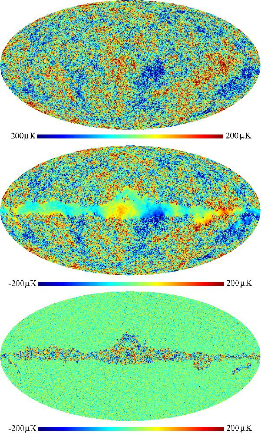
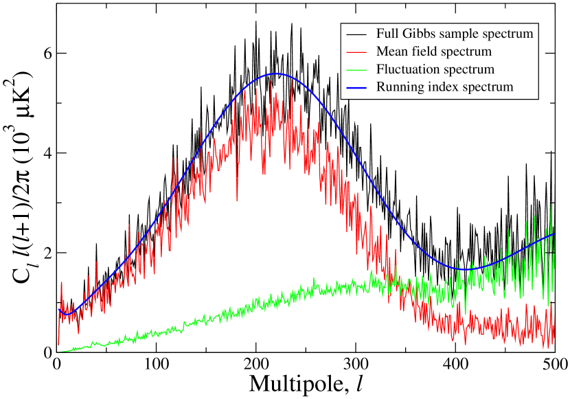
Examples of such maps are shown in figure 1, and the corresponding power spectra are shown in figure 2. However, in practice the two equations are solved simultaneously by solving for the sum of and , in order to reduce the total CPU time.
Finally, we point out that even though the Gibbs sampling technique is a Bayesian method, a frequentist view may be taken by choosing a uniform prior. In that case, the procedure reduces to simply exploring the joint likelihood, and frequentist concepts such as the maximum likelihood estimate may be established.
2.2. Consistent treatment of mono- and dipole contributions
One of the most elegant features of this formalism is its ability to incorporate virtually any real-world complication, as discussed by Jewell et al. (2004) and Wandelt et al. (2004). A few examples of this flexibility are applications to noise, asymmetric beams, non-cosmological foregrounds, or arbitrary sky coverage. However, in this paper we include only the effects of the mono- and dipole contributions (which may be thought of as foregrounds) and that of partial sky coverage, given that our main scientific goal is to analyze the fairly well-behaved WMAP data.
The question regarding mono- and dipole contributions has gained renewed importance during the previous year, given the very active debate concerning the quadrupole seen in the WMAP data. This quadrupole appears to be small compared to the best-fit cosmological model (Spergel et al., 2003; Efstathiou, 2003a; de Oliveira-Costa et al., 2004), and several authors have considered what this may imply in terms of new physics. However, the exact significance of this anomaly is difficult to assess for several reasons, but mainly because of uncertainties in the foreground subtraction process (Eriksen et al., 2004; Slosar & Seljak, 2004). Methodology issues for estimating the lowest multipole amplitudes have also been pointed out (Efstathiou, 2003b). Strongly related to both these issues is the fact that non-cosmological mono- and dipole contributions may couple into the other low-order modes through incomplete sky coverage.
The most common way of handling this latter problem is to fit a mono- and dipole to the incomplete sky, including internal coupling caused by the sky cut, and then simply subtract the resulting best-fit components from the data. However, this procedure neglects the noise correlations that are introduced by removing any fitted templates. The Gibbs sampling framework allows a statistically more consistent approach: rather than directly subtracting the fitted mono- and dipoles from the data, one may marginalize over them through sampling, and thus recognize the inherent uncertainties involved.
As always in Bayesian analyses, one has to choose a prior, and the most natural choice in this case is a uniform prior. This corresponds to saying that we do not know anything about these components. For analytic computations and proofs, however, it is more convenient to define this as a Gaussian with infinite variance, which is just a different way of parameterizing a uniform prior. It should be noted that a uniform prior does not mean that these components are unrestricted, but, rather, it simply means that their values are determined by the data alone.
Again, general formalisms for handling this type of problem were described by Jewell et al. (2004) and Wandelt et al. (2004), and we will only repeat the operational steps here, in a notation suitable for our purposes. Let us first define a template matrix containing the four real spherical harmonics in pixel space,
| (7) |
where and
| (8) | ||||
| (9) | ||||
| (10) | ||||
| (11) |
Note that is a projection matrix onto the subspace spanned by the corresponding templates.
Next we define a vector of template amplitudes , letting the amplitudes be different for each channel, since we have no reason to assume that these components are frequency independent. Thus, the mono- and dipole contribution to the th channel is .
We now want to sample from the conditional distribution , and this is done (assuming the infinite variance prior) by solving the following equation,
| (12) |
where the mono- and dipole residual map is , and
| (13) |
Here, are white noise maps of vanishing mean and unit variance.
The next step in traditional Gibbs sampling would now be to sample from the conditional density , where are the parameters of the probability distribution describing the mono- and dipoles. However, since we have chosen a very special prior, namely one with infinite variance, this distribution does not change, and no sampling is required.
Including the mono- and dipole components in the Gibbs sampling chain, it now reads
| (14) | ||||
| (15) | ||||
| (16) |
The first step is computed as described in the previous paragraphs, and the second step is computed by equation 5, with the slight modification that the mono- and dipole contributions now are subtracted from the data, .
2.3. Incomplete sky coverage
Perhaps the single most important complication in any CMB analysis is proper treatment of foregrounds. With amplitudes up to several thousand times the CMB amplitude, Galactic foregrounds will necessarily compromise any cosmological result unless corrected and accounted for. Unfortunately, there is currently a critical shortage of robust component separation (or even just foreground removal) methods, and the only reliable approach at the time of writing is simply to mask out the most contaminated regions of the sky. On the bright side, the flexibility in specifying foreground models that can be implemented in the Gibbs sampling approach offers an attractive avenue for progress. This will be explored further in future publications.
The Gibbs sampling approach supports two fundamentally different methods for removing parts of the sky by means of a mask. First, the most straightforward option from a conceptual point of view is simply to set the inverse noise matrix to zero at all pixels within the mask. This corresponds to saying that the noise level of these pixels is infinite, and therefore that the data are completely non-informative. No other modifications of the equations are necessary. This is the solution chosen for the Commander implementation.
However, this approach carries a considerable cost in the form of a poorly conditioned coefficient matrix , which, as we will discuss at greater length in the next section, results in slow convergence for the conjugate gradient algorithm, and increased overall expense for the Gibbs sampling. Recognizing this fact, an alternative approach was chosen for the MAGIC implementation, namely to introduce a new foreground component into the Gibbs sampling chain.
Let us recall the general sampling equation for the foreground component (Wandelt et al., 2004),
| (17) |
Here is the covariance matrix for the foreground prior, is the residual map after removal of the signal estimate and any other foregrounds already sampled by the algorithm, and are vectors of uniform Gaussian variates. Finally, is the unconvolved foreground sample.
For each pixel in the masked region, mainly the Galaxy but also some point sources, we do not know the foreground contribution. The maximally uninformative foreground prior for these pixels has infinite variance. It corresponds to a complete lack of a priori knowledge of the foregrounds in the mask. By specifying maximal ignorance of the foreground we allow the algorithm to determine the level of the foreground in these pixels which is supported by the data. Substituting this foreground prior into equation 17 creates a method to numerically marginalize over the unknown foreground contribution in the masked pixels.
In the limit of ’infinite’ variance, this sampling equation simplifies to
| (18) |
in the masked region and outside. This is easy to compute and avoids the use of the Conjugate Gradient solver, hence saving computational time.
With the introduction of this foreground component, the full Gibbs chain reads
| (19) | ||||
| (20) | ||||
| (21) | ||||
| (22) |
Again, the only modifications in the two middle steps is a subtraction of the foreground components from the corresponding residual maps, and .
As mentioned earlier, the main advantage of this approach is that the uniform properties of the coefficient matrix are conserved, leading to a faster convergence for the conjugate gradient solver, often reducing the number of iterations by a factor of three. On the other hand, there is also a slight disadvantage in that the correlations between consecutive Gibbs samples are stronger, since information is carried over from sample to sample through the foreground component. However, this is more than compensated by the rapid CG convergence. We will return to these issues later.
3. Computational considerations
3.1. Conjugate gradients and preconditioning
As described in section 2.1, equations 5 and 6 are the very heart of the Gibbs sampling method, and its feasibility is directly connected to our ability to solve those equations. For a low-resolution experiment such as COBE-DMR, which comprises a few thousand pixels or multipole components, the system may be solved directly, for instance through Cholesky decomposition. However, for a high-resolution experiment such as WMAP, with eight cosmologically important maps of each several millions pixels, more sophisticated algorithms must be employed, and the most efficient method currently available for positive-definite matrices is the Conjugate Gradient (CG) method (Golub & van Loan, 1996). For a truly excellent review of this algorithm, see Shewchuk (1994).
The general problem is to solve a system of linear equations,
| (23) |
where the coefficient matrix is very large. In the case of the first-year WMAP data, corresponds to a system of three million equations in pixel space, and a system of several hundred thousands equations in harmonic space (depending on the of choice; see section 4.1.2 for a discussion on how to choose an appropriate ). Further, this coefficient matrix is in general not sparse in either real space due to complicated signal correlations, or in harmonic space due to complicated noise correlations. However, favorable sparsity patterns may be obtained for special scanning strategies and sky cuts (Oh et al., 1999; Wandelt & Hansen, 2003).
For this reason, the sheer size of the problem poses a real problem, and for many applications one may find that the system described above is ill-conditioned. For instance, the solution vector contains elements of very different magnitudes, and therefore round-off errors can easily compromise the results. It is therefore numerically advantageous to rewrite equations 5 and 6 as follows,
| (24) | ||||
| (25) | ||||
The coefficient matrix is now much better behaved, and all elements of the solution vector have unity variance. Note also that the diagonal elements of are now simply the signal-to-noise ratios of the corresponding mode.
We choose to work in harmonic space in the following for several reasons. First, in this space it is easy to limit the size of the problem according to the signal-to-noise ratio of the data by choosing an appropriate . In pixel space one is always forced to work with vectors of length . Second, given the form of equations 5 and 6, two spherical harmonics transforms are eliminated by operating in harmonic space in the first place, thereby reducing the total CPU time by a factor of two. Finally, since we are mainly interested in the power spectrum, an harmonic space based convergence criterion for the CG search seems more natural than a pixel space based criterion.
One of the main advantages of the CG algorithm is that it does not require inversion of the coefficient matrix, and we do not even need to store it. All we need is the ability to multiply with a given vector , and solving a preconditioning equation. We first consider the matrix multiplication operation. In our setting, for which , this is done in a step-wise fashion. First we multiply each component of the input vector by (where is the product of the beam and pixel window functions), and then we perform an inverse spherical harmonic transform into real space. Here we multiply with the inverse noise matrix, , under the assumption of uncorrelated noise. Then we perform an ordinary spherical harmonic transform of the vector into harmonic space, where we again multiply with the beam and square root of the power spectrum. Finally we add the original vector. Thus, multiplication of is computationally equivalent to two spherical harmonic transforms, and memory requirements are virtually negligible444If accessible memory is sufficient on the available computer, one may want to precompute the associated Legendre polynomials, reducing the total CPU time typically by a factor of two or three for WMAP type maps in the current HEALPix implementation. The memory requirement for doing so is bytes, or on the order of 1GB for , being the HEALPix resolution parameter, which corresponds directly to the number of pixels in the map through the relation ..
The efficiency of the CG algorithm is highly dependent on our ability to construct a good preconditioner (e.g., Oh et al. 1999), and two preconditioners have been proposed for this problem so far, both approximating in harmonic space. First, under the assumption of white, but non-uniform, noise, the inverse real-space noise covariance matrix may be written as a simple inverse noise rms map, , which again may be expanded into spherical harmonics,
| (26) |
The inverse noise matrix in spherical harmonic space is then (Hivon et al., 2002)
| (27) |
A very simple preconditioner may therefore be defined in terms of the diagonal elements only,
| (28) |
While satisfactory for the simplest applications, we find that it takes about 300 iterations to solve for the WMAP data consisting of all eight cosmologically interesting bands with this preconditioner (applying the Kp2 mask directly), making the total solution of the problem very expensive.
By considering the overall structure of the inverse noise matrix, Oh et al. (1999) proposed to use a block-diagonal matrix. In the limit of perfect azimuthal symmetry of both the galactic cut and the noise distribution, is orthogonal with respect to , and therefore it makes sense to also include all elements having up to some arbitrary limit . At higher ’s, the diagonal preconditioner is used. Oh et al. (1999) claims to achieve convergence in six iterations with this preconditioner for properties corresponding to the two-year WMAP data, but, unfortunately, we have not yet been able to reproduce this performance. From our experiments it seems the combination of a highly non-symmetric Kp2 cut, 700 resolved point source cuts, and a noise distribution tilted with respect to the galactic plane introduces significant couplings between different ’s.
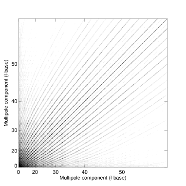
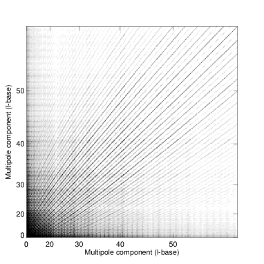
In figure 3 we have plotted the coefficient matrices corresponding to the first-year WMAP data in two different orderings, both -major and -major (see caption for details), and with and without application of the Kp2 mask. In the limit of uniform noise and no galactic cut, these matrices would all be diagonal, and convergence would be reached in one single CG iteration using even the diagonal preconditioner.
However, as seen in the top two panels of figure 3, adding non-uniform noise to the problem introduces significant coupling between different modes, which again leads to poorer CG performance. In the left panel, we see that the largest absolute values are found at low ’s, which of course is not very surprising, considering that these matrices are a measure of the signal-to-noise ratio. In the right panel we see the same matrix organized as -major, and in the limit of azimuthal symmetry, this would be a strictly block-diagonal matrix with very small block elements. The preconditioner proposed by Oh et al. (1999) consists of the inverses of those blocks. But, as we see, there are many off-diagonal elements in this matrix, and, indeed, the dominant elements actually seem to be components for which . However, if we had computed these quantities in the ecliptic frame, rather than in the galactic, then the matrix is likely to be dominated by the elements, and possibly even by the elements.
The bottom two panels show a similar set of matrices, but in this case the Kp2 mask has been applied to the sky. And, as mentioned in section 2.3, this has the highly undesirable effect of magnifying the off-diagonal elements through mode-to-mode coupling considerably. Unfortunately, neither of these matrices have a very dominant symmetry structure, and it is therefore difficult to establish an optimal preconditioner.
Nevertheless, based on the structures seen in the lower left panel in figure 3 a third alternative was chosen for the Commander implementation. Rather than including only the diagonal elements, or only elements as Oh et al. (1999) do, we include all elements up to some arbitrary (typically –70 for WMAP), and at higher ’s we include only the diagonal elements. The required memory requirements for this matrix scales as , and are thus quite expensive, but in practice, the real limitation is the CPU time required for its Cholesky decomposition (which scales as ) rather than memory requirements for its storage. For , the memory requirements are 52 MB and the CPU time for Cholesky decomposition is on the order of one or two minutes. Obviously, the latter number must be compared to the CPU time it takes to perform one CG iteration and the number of iterations saved. And yet, even with this rather expensive preconditioner, we find that the CG search converges in about 60 iterations for the combined first-year WMAP data and a norm-based fractional convergence criterion of . Thus, our performance is not as impressive as the six iterations achieved by Oh et al. (1999). Work on this issue is still on-going, and a hybrid of all three variants may prove to be the ultimate solution.
In contrast to the Commander implementation, MAGIC does not apply a sky cut directly, but instead it introduces a new random field into the sampling chain. The appropriate coefficient matrix is therefore the one shown in the upper left panel of figure 3. This choice has a very positive effect in terms of CG performance, and one routinely achieves convergence within 20 iterations using just the simple diagonal preconditioner for a first-year WMAP type experiment. However, as we will see later, the cost for this performance comes in the form of a slightly longer correlation length in the Markov chain, and therefore fewer independent samples.
3.2. Parallelization
The main limitation for the Gibbs sampling method is CPU time. Even though the scaling of the method is equivalent to that of a spherical harmonics transform for a WMAP type analysis, one has to perform this operation many times, and the total prefactor of the algorithm is therefore large. Specifically, the number of spherical harmonic transforms to produce one Gibbs sample is two times the number of CG iterations, times the number of frequency bands. The total number of transforms for computing one sample from an eight-band WMAP data set is then typically on the order of 1000 for the Commander approach (reaching convergence in 60 iterations) and 350 for the MAGIC approach (reaching convergence in 20 iterations). Knowing that one harmonic transform takes about 5 seconds for and , the total CPU time required for one single Gibbs sample is therefore on the order of one or two hours for Commander and half an hour for MAGIC. Obviously, parallelization is essential to produce a sufficient number of samples.
Two fundamentally different approaches may be taken in this respect. Either one may choose to run one single Markov chain and parallelize the spherical harmonic transforms internally. Since the HEALPix routines operate on pixel rings of constant latitude, this can be done quite efficiently by letting each processor compute its own ring. Nevertheless, optimal speed-up will not be achieved, and the implementation will be somewhat complicated.
The other approach is to take advantage of the fact that this method is truly a Monte Carlo method, and one can therefore let each processor run its own Markov chain. The most important advantages of this approach are optimal speed-up and the possibility to initialize each chain with a different first guess. As we will see in the next section, consecutive Gibbs samples in the Markov chain are highly correlated in the low signal-to-noise regime, and producing a larger number of independent samples is therefore quite expensive. If we have a rough approximation of the true spectrum and its uncertainties (as we usually do, through a MASTER type analysis; Hivon et al. 2002), we can partially remedy this problem by initializing each Markov chain with an independent power spectrum.
The major drawback of this latter parallelization scheme, however, is that each Markov chain will necessarily be quite short, perhaps only twenty to fifty samples. This problem is due to the fact that most current super-computer facilities have a maximum wall-clock time limit of 24 to 72 hours, and therefore the maximum length of one chain is on the same order of magnitude. Of course, one may store intermediate results and restart the computations after every cycle, but this only increases the total length by a factor of a few, not by hundreds.
We have chosen a combination of external and internal parallelization in our implementation, by recognizing the fact that we will in general be analyzing multi-frequency data sets consisting of maps. We may therefore let processors work on the same Markov chain, each processor transforming one band. Thus, optimal speed-up is not compromised, while the length of the chains is increased by the same factor. In future versions we will also implement fully internal parallelization in the HEALPix routines map2alm and alm2map, to have the option of focusing all the computational resources into one single chain.
4. Simulations
In this section we apply the Commander and MAGIC codes to simulated data sets for which all components are perfectly known. The goals are two-fold. Firstly, we wish to demonstrate that the codes produce results consistent with theoretical expectations, and secondly, we seek to gain insight on what limitations of the algorithm we can expect to meet in real-world applications, when CPU time is limited.
A number of different simulations are analyzed in the following sections, each designed to highlight some specific feature. First, in order to establish the asymptotic behavior of the algorithm, we study a data set of smaller size than the full-resolution WMAP data. Specifically, we construct a data set at intermediate resolution (; 196 608 pixels), for which the CPU time per sample is on the order of 10 seconds. Thus, CPU time is not a dominating problem, and we can establish the Markov chain correlation lengths and power spectrum correlation matrix to great accuracy. The burn-in time is also considered.
Finally, we make two simulations at full WMAP resolution in order to confirm that the overall results from the low-resolution analysis carry naturally over to higher resolutions. This time the CPU cost is the limiting factor, and the main goal of this section is in fact to demonstrate that the Gibbs sampling method is able to handle even large data sets, such as the WMAP data. This analysis mimics the analysis of the first-year WMAP data presented by O’Dwyer et al. (2004), in that it is run on a super-computer with many short, parallel chains. The only difference between the two runs is that either white or correlated noise are added to the CMB simulations. This way we test whether the assumption of white noise may compromise the scientific results in the presence of small, but non-negligible, noise correlations. We find that this is not a significant problem for the first-year WMAP data.
4.1. Low-resolution simulations
The main goal of the low-resolution simulations is to study the asymptotic behavior of the method when the number of independent samples is very high. On the one hand, this allows us to verify that the codes work as expected without worrying about errors introduced because of a limited number of samples, and on the other, essential quantities such as the Markov chain correlation length and the power spectrum correlation matrix may be established to a high degree of accuracy.
In order to facilitate such long-chain analyses, we study maps with relatively low resolution, , but with properties corresponding to a consistently down-scaled WMAP-type experiment. Specifically, we generate a CMB sky from the best-fit WMAP running index spectrum, and convolve this sky with modified version of the WMAP beams. The beams are made four times wider by replacing their original Legendre transform with .
The noise components are generated by degrading the original WMAP noise rms maps555The noise rms maps are defined by , where is the average sensitivity of the various bands, and is the number of observations for each pixel . to by simple averaging over pixels in the HEALPix nested organization. Thus, the noise per low-resolution pixel in our simulated maps is about the same as that for each high-resolution pixel in the full-sized WMAP data. The signal-to-noise ratio is therefore downscaled to the appropriate resolution, a fact which will be important when studying the relationship between the correlation length and the signal-to-noise ratio.


We also want to study the effect of residual mono- and dipoles on the cosmological power spectrum, and we therefore add a random mono- and dipole contribution with an artificially large amplitude (on the order of tens to a hundred mK) to the signal plus noise map. The reconstructed values are then later compared with the exact input values.
Finally, we generate a degraded mask to match this resolution, based on the WMAP Kp2 mask as defined by Bennett et al. (2003b). This mask is downgraded to by requiring that all high-resolution sub-pixel within a pixel (again, in the HEALPix nested organization) are included by the original mask. Thus, this mask is very slightly expanded compared to the actual Kp2 mask.
4.1.1 Verification of algorithms and codes
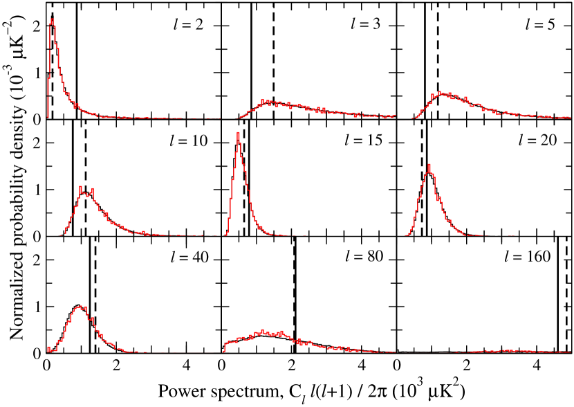
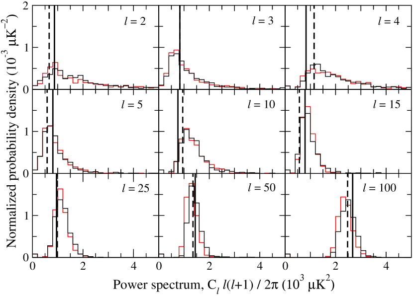
In the first test, we apply the Commander and MAGIC codes to one single band from the data set described above, namely to the V1 band. Commander was run for 100 000 samples, while MAGIC was run for 4000, with the main goal of comparing the codes, verifying that they produce identical output.
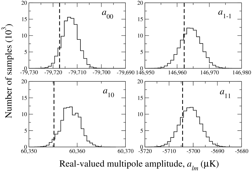
The results from this exercise are shown in figure 4. The black probability densities show the Commander results, while the red histograms show the MAGIC results. The agreement is striking, and this is a strong confirmation that the codes work as expected, and that the minor differences in implementational details discussed earlier do not affect the scientific results.
The dashed lines show the true, underlying CMB power spectrum value, which should theoretically coincide with the peaks of the histograms, in the limit of full sky coverage and no noise. At low ’s, we see that this is indeed the case. Here it is also worth recalling that we added artificially large mono- and dipole components to the simulations (several orders of magnitudes larger than what is realistic), and this does still not compromise the results.
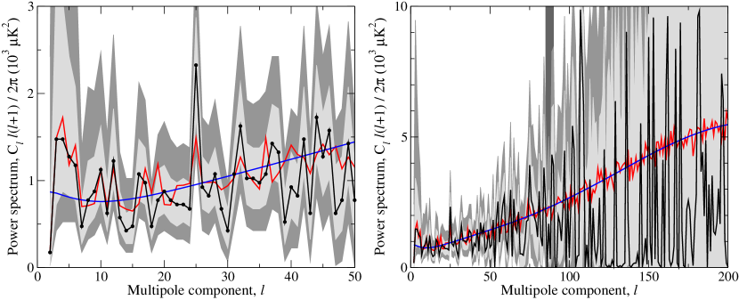
In figure 5 we have plotted the full spectrum computed from the 100 000 sample run. The input spectrum is marked in red, the ensemble-averaged spectrum in blue, and the maximum likelihood solution from the Gibbs sampler in black. The gray bands indicate 1 and confidence regions for the power spectrum.
At low ’s the discrepancy between the estimated and input spectra is primarily due to the galactic cut, while at high ’s it is primarily due to noise. In particular, we see that the maximum likelihood estimate actually drops to zero for many of the low signal-to-noise ratio modes, which, again, is the expected behavior for a maximum likelihood estimator in the noise-dominated regime.
In figure 6 we plot two different correlation matrices, each on the form
| (29) |
The averages are taken over the 100 000 samples in the Markov chain described above. The left panel shows the correlation matrix of the sampled power spectra, which are basically uncorrelated by construction, while the right panel shows the correlation matrix of the power spectra, , computed from the sampled maps, . The latter matrix is related to the correlation matrix of the maximum likelihood power spectrum found by maximizing the posterior, and mainly describes mode-mode coupling due to the cut sky on these scales.
Finally, in figure 7 we plot the distributions of the mono- and dipole samples and compare them to the input values, marked by dashed, vertical lines. Although there certainly is a discrepancy between the distribution modes and the input values, the overall rms values are very small, on the order of 5–, and consistent with the fluctuation level expected for a single realization. Further, there is some coupling between the mono- and dipole modes due to the galactic cut, which could be important. However, since our sole interest in these components lies in removing them, rather than estimating them, this is not an important problem for our purposes. In fact, given the very small impact of these very large mono- and dipole components, we feel confident that the cosmological low- spectrum is not compromised by mono- and dipole issues.
4.1.2 Convergence and correlations
We now turn to the issues of convergence, correlation length and burn-in time, all of which must be thoroughly understood in order to design and optimize a real-world analysis properly. The problem can be plainly stated as follows: How many Gibbs samples do we need to estimate the power spectrum with sufficient accuracy in order to be limited by non-algorithmic issues? As we will see, the answer depends intimately on which angular scales we wish to consider, a conclusion which is most easily seen by going back to the Gibbs sampling scheme.
The algorithm works as follows: First we assume some arbitrary (but hopefully reasonable) power spectrum, and compute a Wiener-filtered map based on that spectrum. Then we add a fluctuation term which replaces the power lost both to noise and to the galactic cut. The sum of those two terms mimics a full-sky, noiseless map with a power spectrum determined by the data in the high signal-to-noise regime, and by the assumed power spectrum in the low signal-to-noise regime. From this full-sky power spectrum we then draw a new spectrum, which subsequently is taken as the input spectrum for the next Gibbs iteration.
The crucial point is that the random step size in the final stage is determined by the cosmic variance alone. Our goal is to probe the full probability distribution which includes both noise and cosmic variance. In the high signal-to-noise regime, the difference does not matter. Sequential Gibbs samples are therefore for all practical purposes uncorrelated. The opposite is true in the low signal-to-noise regime: since the distance between the two samples is determined by the cosmic variance, while the full distribution is dominated by the much larger noise variance, two sequential samples will be strongly correlated.
This problem is a severe limitation for the Gibbs sampling technique in its current formulation. It makes it very expensive to probe the low signal-to-noise regime completely. The Gibbs sampling technique is only a special case of the more general Metropolis-Hastings framework. Other sampling schemes may be devised which break the correlation between neighboring samples. This will be the topic of a future publication, and for now our main goal is to quantify this effect, rather than eliminate or minimize it.
We take advantage of the low-resolution simulations in order to quantify these correlations. Specifically, we consider the power spectrum values at constant in the Markov chain as independent functions, and study the correlations in these chains as a function of . The statistic we choose for this study is a simple auto-correlation function,
| (30) |
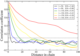
Here is the distance in the chain measured in number of iterations. Such functions are plotted in figure 8 for six different ’s, computed from a new Commander chain consisting of 3800 samples, including all eight bands.
As expected, the correlations become stronger as increases, or, equivalently, as the signal-to-noise ratio decreases. In this particular case, the signal-to-noise ratio is unity at approximately , and therefore the spectrum is limited by cosmic variance at smaller ’s. This translates into a very short correlation length for in this case, and consequently into a high efficiency in terms of independent samples. On the other extreme, the correlation length at is very, very long, and with only 3800 samples in the chain, we have only a very few independent samples from which to form our power spectrum estimate.
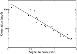
We can take this exercise one step further and define a typical correlation scale for each , by computing the scale at which the correlation function drops under, say, 0.1. In figure 8 we have plotted this correlation length directly as a function of the signal-to-noise ratio, and from this plot there seems to be a well-defined relationship between these two quantities. In fact, we will use this relation to estimate how many samples we need in the actual WMAP analysis later on. For now we note that with 3800 samples, as in the above case, we have about 200 independent samples at a signal-to-noise ratio of 0.6, which corresponds to . In other words, it would be rather optimistic to believe in the power spectrum based on these samples at ’s higher than, say, 110.
Another lesson to be learned from these plots is that the correlation length increases very rapidly with , once entering the low signal-to-noise regime. This is an important point to realize when desiging a new analysis: probing the low signal-to-noise regime with the current implementation of the Gibbs sampling algorithm is extremely expensive. It may therefore often be desirable to limit to the corresponding to a signal-to-noise ratio of, say, 0.5 or 0.25. The saved CPU time666The algorithm scales overall as . may then be spent on producing more independent samples in the high and intermediate signal-to-noise regimes. However, truncating the system this way does modify the global solution, and care must therefore be taken with respect to the highest ’s. In general, the larger the sky cut, the more high- modes will have to be discared from the final power spectrum, since mode-mode couplings spread the sharp -space cut-off into a wide range of multipoles. In practice, it is convenient to pre-define some range of ’s of interest, and then increase until that range becomes stable.
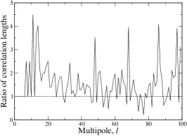
In figure 8 we have plotted the ratio of the MAGIC correlation length to the Commander correlation length, and here it is seen, as noted earlier, that the MAGIC correlation length is typically a factor of 1.5–2 longer at low ’s, resulting in a smaller number of independent samples of the same factor. Of course, this is both caused and made up by the fact that MAGIC handles the incomplete sky coverage differently than Commander. Since MAGIC obtains convergence in the CG search roughly three times faster than Commander (using a very crude preconditioner), the codes do perform quite similarly in terms of total CPU time per independent sample.
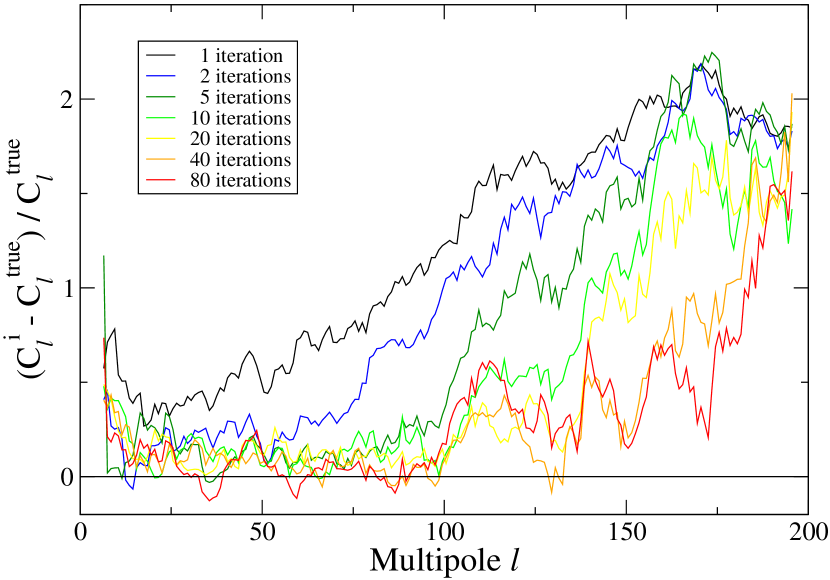
Finally, we turn to the issue of burn-in time. Although the theory of Gibbs sampling guarantees us that the samples will converge toward being samples from the joint distribution density, it does not tell us when such convergence is obtained, and this must therefore be established by experiments. We study this issue through a simple exercise: Once again we utilize the simulated data described above, but this time we choose a first power spectrum guess which is exactly three times larger than the true spectrum. Then we run the algorithms for a number of iterations, and plot the power spectrum samples as a function of iteration count, . The results from this exercise are shown in figure 9, in the form of
| (31) |
Note that the spectra have been averaged with a window width of , making it easier to see the overall trends.
The conclusion to be drawn from this plot seems clear: A poor initial guess can invalidate a large number of samples, and, in particular, a weak estimate of the low signal-to-noise regime is very expensive to correct. This can potentially pose a serious threat to our main parallelization scheme, which is based on many independent short chains, rather than one long chain. For this reason, the Gibbs sampling approach in its current form may not be particularly well suited as the only estimator for a new experiment. A faster method, such as Master (Hivon et al., 2002), is therefore suggested to provide an initial guess for the Gibbs samplers. Once an approximate power spectrum is established, the Gibbs sampling process is already within the appropriate range, and only a few samples need to be discarded, if any at all. However, we do not need to rely blindly on the first guess, since a poorly chosen starting point would lead to a systematic drift in the Gibbs chains which should be easily detectable.
4.2. High-resolution simulations
In this section we turn to high-resolution simulations, and undertake a full-scale WMAP-type analysis. The simulations in this case are prepared in the same way as in the low-resolution case, except with full-scale input data, and no inclusion of mono- and dipole components.
The main limitation in this case is CPU time, and extremely long chains are simply not feasible. Instead, we run many independent chains in parallel, each producing only a small number of samples, as discussed in section 3.2.
The analysis is designed to match the analysis of the first-year WMAP data presented by O’Dwyer et al. (2004). Specifically, we generate a random sky with the HEALPix utility synfast, and convolve this sky with the beams corresponding to each of the eight WMAP bands (Q1–2, V1–2, W1–4). Next we add either white noise (with the appropriate patterns for each band) or correlated noise (as generated by the WMAP team777Available at http://lambda.gsfc.nasa.gov.) to these CMB maps. Finally, the WMAP Kp2 mask (Bennett et al., 2003b) which excludes point sources is imposed on the data, leaving 85% of the sky available for analysis. At this stage, the Gibbs sampler is run over 12 independently initialized chains for 60 iterations, for a total of 720 samples.
We point out that the numbers of observations per pixel, , in the correlated noise files supplied by the WMAP team do not match perfectly those of the observed map files, and unless the appropriate patterns are used in each case, a noise excess at is observed. The white noise level, however, are identical for the two patterns, and so this difference does not have a significant impact on the results, as long as one is aware of the difference.
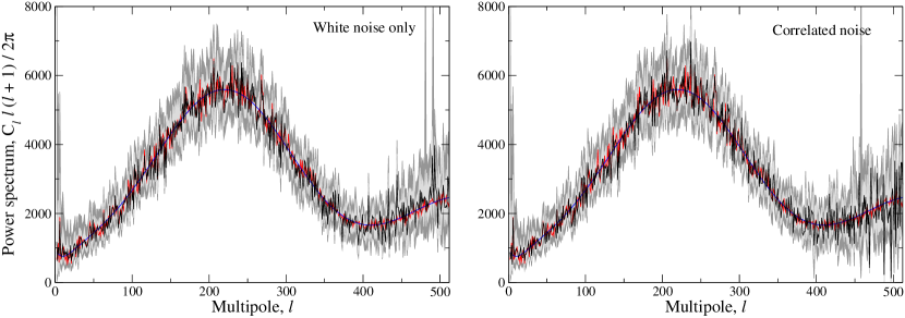
In figure 10 we have plotted the power spectra from the multiple-chain analysis, including white noise in the left panel and correlated noise in the right panel. Overall, we see that the agreement between the realization specific spectrum (red line) and the maximum likelihood solution (black line) found by the Gibbs sampler is quite good, and there is no detectable bias in any parts of the spectrum.
Next, in figure 11 we plot a few selected histograms of the power spectra, comparing the white (black histograms) and correlated (red histograms) noise results more directly. As we see, the agreement is generally very good, and in particular, the three upper panels clearly demonstrate that the low level of correlated noise present in the WMAP data do not compromise the low- spectrum.
At higher ’s, a small shift may be seen between the two distributions, which is most likely due to the fact that the noise realizations are different. We made similar plots for neighboring multipoles, finding that the absolute levels of discrepancy seen in figure 11 are quite typical for these angular scales, and the signs of the shifts are random. Thus, the differences does not seem to be indicative of a systematic bias.
By studying simulated data, we have thus explicitly demonstrated that the Gibbs sampling technique is able to analyze the mega-pixel WMAP data set properly, and that neither correlated noise nor incomplete sky coverage compromise the scientific results significantly. All in all, the feasibility of this approach with respect to current and future data sets has been firmly established.
5. Conclusions
We have implemented two independent versions of the Gibbs sampling technique introduced by Jewell et al. (2004) and Wandelt et al. (2004), and tested the performance and behavior of the codes thoroughly. In particular, we have explicitly verified that the two implementations produce identical output, despite a few algorithmic differences, demonstrating that these algorithmic choices do not affect the scientific results. Further, we applied the codes to simulated data with controlled properties, and found the output to agree very well with the theoretical expectations. In doing so, we also demonstrated the feasibility of the method for high-resolution applications.
One of the main goals of these simulations was to build up intuition about the phenomenological behavior of the Gibbs sampling algorithm, focusing in particular on issues such as the correlation length of the Markov chains, and the burn-in and convergence time. Through these experiments, we found that the signal-to-noise ratio is by far the most constraining factor to the algorithm in its current form. The step size between two consecutive samples is determined by the cosmic variance alone, while the overall posterior density incorporates noise uncertainty as well. Thus, in the low signal-to-noise regime subsequent samples are highly correlated, and the effective number of independent samples is dramatically reduced. In its current formulation, the method is therefore most efficient at scales for which the signal-to-noise ratio is higher than, say, 0.5, or perhaps up to –400 for the first-year WMAP data. On the other hand, the Gibbs sampler is only a special case from a more general framework, and other sampling schemes may be introduced in order to break these correlations. This will be the topic of a future publication.
Perhaps the single most appealing feature of the Gibbs sampling approach, is its ability to incorporate most real-world complications in a statistically consistent manner. In this paper we have demonstrated how to handle incomplete sky coverage and unknown mono- and dipole contributions, which are the most important point for the analysis of the first-year WMAP data, but future extensions will also include polarization, more sophisticated treatment of foregrounds, internal sampling over cosmological parameters, inclusion of asymmetric beams, and statistically consistent handling of noise. In fact, the Gibbs sampling approach is not simply a maximum likelihood method, but rather a machinery facilitating an optimal, global analysis. Needless to say, the computational challenges are considerable, but with a scaling equivalent to that of map making (which has to be performed in any approach currently proposed), this method may just be able to do the job.
A second goal of this paper was to prepare for the actual analysis of the WMAP data, by applying the algorithm to simulated data with similar properties. Specifically, we showed that the estimated power spectrum is unbiased, and that even the lowest-order multipoles are not compromised by the either the galactic cut, given that the foreground correction method presented by Bennett et al. (2003a) is adequate, or by the (low levels of) correlated noise present in the data. Thus, no further sophistications beyond those presented in this paper seem necessary in order to perform a valid Bayesian analysis of the first-year WMAP. The scientific results from this analysis are presented in a companion letter by O’Dwyer et al. (2004).
References
- Bennett et al. (2003a) Bennett, C. L. et al. 2003a, ApJS, 148, 1
- Bennett et al. (2003b) Bennett, C. L. et al. 2003b, ApJS, 148, 97
- Bond, Jaffe & Knox (1998) Bond, J. R., Jaffe, A. H., & Knox, L. 1998, Phys. Rev. D, 57 2117
- Borrill (1999) Borrill, J. 1999, Phys. Rev. D, 59, 027302
- Challinor et al. (2002) Challinor, A. D., Mortlock, D. J., van Leeuwen, F., Lasenby, A. N., Hobson, M. P., Ashdown, M. A. J., & Efstathiou, G. P. 2002, mnras, 331, 994
- de Oliveira-Costa et al. (2004) de Oliveira-Costa, A., Tegmark, M., Zaldarriaga, M., & Hamilton, A. 2004, Phys. Rev. D, 69, 063516
- Doré, Knox & Peel (2001) Doré, O., Knox, L., & Peel, A. 2001, Phys. Rev. D, 64, 083001
- Efstathiou (2003a) Efstathiou, G. 2003a, MNRAS, 343 L95
- Efstathiou (2003b) Efstathiou, G. 2003b, MNRAS, 346, L26
- Eriksen et al. (2004) Eriksen, H. K., Banday, A. J., Górski, K. M., & Lilje, P. B. 2004, ApJ, in press, [astro-ph/0403098]
- Górski (1994) Górski, K. M. 1994 ApJ, 430, L85
- Górski (1996) Górski, K. M. 1997, preprint [astro-ph/9701191]
- Górski et al. (1999) Górski, K. M., Hivon, E., & Wandelt, B. D., 1999, in Evolution of Large-Scale Structure: from Recombination to Garching, ed. A. J. Banday, R. K. Sheth, & L. N. da Costa (Garching, Germany: European Southern Observatory), 37
- Golub & van Loan (1996) Golub, G. H. & van Loan, C. F. 1996, Matrix Computations, The Johns Hopkins University Press
- Hansen & Górski (2003) Hansen, F. K., & Górski, K. M. 2003, MNRAS, 343, 559
- Hansen, Górski & Hivon (2002) Hansen, F. K., Górski, K. M., & Hivon, E. 2002, MNRAS, 336, 1304
- Hinshaw et al. (2003) Hinshaw, G. et al. 2003, ApJS, 148, 135
- Hivon et al. (2002) Hivon, E., Górski, K. M., Netterfield, C. B., Crill, B. P., Prunet, S., & Hansen, F. 2002, ApJ, 567, 2
- Jewell et al. (2004) Jewell, J., Levin, S., & Anderson, C. H. 2004, ApJ, 609, 1
- O’Dwyer et al. (2004) O’Dwyer, I. J. et al. 2004 ApJ, submitted [astro-ph/0407027]
- Oh et al. (1999) Oh, S. P., Spergel, D. N., & Hinshaw, G. 1999, ApJ, 510 551
- Page et al. (2003) Page, L., et al. 2003, ApJS, 148, 39
- Shewchuk (1994) Shewchuk, J. R. 1994, http://www.cs.cmu.edu/quake-papers/painless-conjugate-gradient.ps
- Slosar & Seljak (2004) Slosar, A., & Seljak, U. 2004, Phys. Rev. D, in press [astro-ph/0404567]
- Spergel et al. (2003) Spergel, D. N. et al. 2003, ApJS, 148, 175
- Tegmark (1997) Tegmark, M. 1997, Phys. Rev. D, 55, 5895
- van Leeuwen et al. (2002) van Leeuwen, F. et al. 2002, MNRAS, 331, 975
- Wandelt (2003) Wandelt, B. D. 2003, eConf, C030908, WELT001, [astro-ph/0401623]
- Wandelt & Hansen (2003) Wandelt, B. D., & Hansen, F. K. 2003, Phys. Rev. D, 67, 023001
- (30) Wandelt, B. D., Hivon, E., & Górski, K. M. 2001, Phys. Rev. D, 64, 083003
- Wandelt et al. (2004) Wandelt, B. D., Larson, D. L., & Lakshminarayanan, A. 2004, [astro-ph/0310080]