New light on Dark Cosmos

Abstract

Recent studies by a number of independent collaborations, have correlated the CMB temperatures measured by the WMAP satellite with different galaxy surveys that trace the matter distribution with light from the whole range of the electromagnetic spectrum: radio, far-infrared, optical and X-ray surveys. The new data systematically finds positive correlations, indicating a rapid slow down in the growth of structure in the universe. Individual cross-correlation measurements are of low significance, but we show that combining data at different redshifts introduces important new constraints. Contrary to what happens at low redshifts, for a fixed $\Omega_{m}$, the higher the dark energy contend, $\Omega_{\Lambda}$, the lower the ISW cross-correlation amplitude. At 68% confidence level, the data finds new independent evidence of dark energy: $\Omega_{\Lambda}=0.42-1.22$ . It also confirms, to higher significance, the presence of a large dark matter component: $\Omega_{m}=0.18-0.34$, exceeding the density of baryonic matter, but far from the critical value. Combining these new constraints with the prior of a flat universe, or the prior of an accelerating universe provides strong new evidence for a dark cosmos. Combination with supernova data yields $\Omega_{\Lambda}=0.71\pm 0.13$, $\Omega_{m}=0.29\pm 0.04$. If we also assume a flat universe, we find $\Omega_{\Lambda}=0.70\pm 0.05$ and $w=-1.02\pm 0.17$ for a constant dark energy equation of state.

1 Introduction

In the last few years a new cosmological scenario with a significant smooth Dark Energy (DE) component has emerged. The Cosmic Concordance Model (CCM, from now on) is a spatially flat universe with baryons ($\Omega_{b}\sim 4\%$), cold dark matter ($\Omega_{CDM}\sim 23\%$) and a significant DE component ($\Omega_{\Lambda}\sim 73\%$). The model is well supported by the supernova type Ia observations (SNIA) (?; ?), observations on large scale structure (LSS) (?; ?) and the cosmic microwave background experiments (CMB), in particular by the recent WMAP experiment (?). The energy density of the universe seems dominated by the unknown DE component, presenting a formidable observational and theoretical challenge. The three key observational probes measure complementary aspects of the cosmological parameter space. The SNIA indicate that the universe is accelerating but present data is degenerate for alternative cosmological scenarios. The LSS observations constrain $\Omega_{m}$ but leave the DE question unanswered. Constraints from primary anisotropies in the CMB indicate that we live in a flat universe but require a prior on the value of the local Hubble rate $H_{0}$(?). Assuming that the universe is well described by a $\Lambda$CDM model, combining all these three observations gives us the cosmological CCM model.

The Integrated Sachs Wolfe effect, ISW, (?) is a direct probe for the (linear) rate of structure formation in the universe. Secondary anisotropies in the CMB appear because of the net gravitational redshifts affecting CMB photons that travel through an evolving gravitational potential $\Phi$. These secondary temperature anisotropies are therefore correlated with local, evolving, structures on large scales. The correlation is negative when structures grow, as increasing potential leaves a cold spot in the CMB sky, and positive otherwise. In a flat universe without DE (Einstein-deSitter, or EdS, model) this cross-correlation is expected to be zero because the gravitational potential remains constant, despite the linear growth of the matter fluctuations.

The rate of structure formation in the universe can also be measured by galaxy peculiar velocities or galaxy redshift distortions, on very large scales through the so-call $\beta$ parameter determination (?; ?). The ISW effect provides an independent and complementary probe of the same effect. Independent, because it uses temperature anisotropies instead of the velocity field, and complementary, because of the different assumptions and systematics that relate measurements with theory. Despite recent advances in the size of galaxy redshift surveys such as SDSS and 2dFGRS, the spectrum of matter fluctuations $P(k)\propto<\delta(k)^{2}>$ is quite difficult to measure directly over very large scales (?; ?; ?). Part of the problem is that matter correlations fall quickly to zero on scales larger than $30$ Mpc/h ($k<0.1$ h/Mpc). In contrast, fluctuations in the gravitational potential go as $\Phi(k)\propto\delta(k)/k^{2}$ and therefore extend over larger distances, which makes the signal more detectable (see also comments to Fig. 4). The ISW cross-correlation traces the gravitational potential, $\Phi$, and thus provides a new window to study the largest structures, extending over several degrees in the sky or tens of Mpc/h at the survey depth.

2 Growth of density perturbations

Gravitational evolution of matter fluctuations, $\delta={\rho/\bar{\rho}}-1$, is dependent on the cosmological model via the evolution of the scale factor $a=a(t)$. Compared to a static background, a rapidly expanding background will slow down the collapse of an over dense region. In the linear regime, a small initial perturbation $\delta_{0}$ grows according to the growth factor $D(t)$:

$$\delta(t)=D(t)~{}\delta_{0}$$ (1)

which, under quite generic assumptions, eg (?; ?; ?), follows a simple harmonic equation:

$${d^{2}D\over{d\eta^{2}}}+\left(2+{\dot{H}\over H^{2}}\right){dD\over{d\eta}}+3c_{1}~{}D=0,$$ (2)

where $\eta=\ln(a)$ is the conformal time and $H=H(\bar{\rho})\equiv\dot{a}/a$ is the background Hubble rate ($\dot{a}$ and $\dot{H}$ are proper time derivatives). For a flat cosmological model with a generic dark energy equation of state

$$p=w(z)\rho$$ (3)

we then have:

$$H^{2}=\left({\dot{a}\over a}\right)^{2}=H_{0}^{2}\left[\Omega_{m}(1+z)^{3}+\Omega_{\Lambda}e^{3\int_{0}^{z}{dz^{\prime}\over 1+z^{\prime}}(1+w(z^{\prime}))}\right]$$ (4)

where $\Omega_{\Lambda}$ and $\Omega_{m}$ are the dark energy and dark matter densities today in units of the critical density $\rho_{c}\equiv 3~{}H^{2}/(8\pi G)$. And $c_{1}$ is given by:

$$c_{1}=-{1\over 2}{H^{2}_{0}\Omega_{m}(1+z)^{3}\over H^{2}(z)}$$ (5)

In this paper we study two cases. A generic (not necessarily flat) $\Lambda$CDM model where DE density is constant over the evolution of the universe $(w=-1)$; and a flat $\Lambda$CDM model with a constant equation of state parameter. For those models we have

$$c_{1}=-(1/2)~{}\Omega_{m}/(\Omega_{m}+\Omega_{\Lambda}a^{3})$$ (6)

One may choose to compare the results to the EdS model: $\Omega_{\Lambda}=0,\ \Omega_{m}=1$, in which case the solution to Eq. (2) is $D\propto a$. This means that $\delta$ grows linearly with the scale factor, $\delta\propto a$, while the corresponding gravitational potential fluctuation, $\Phi\sim\delta/a$, remains constant as the universe expands. For non EdS models $\Phi$ would change during the expansion of the universe which would turn into a galaxy-CMB temperature cross-correlation signal.

2.1 The ISW effect

ISW temperature anisotropies are given by (?):

$$\triangle_{T}^{ISW}(\hat{n})\equiv{T(\hat{n})-T_{0}\over{T_{0}}}=-2\int dz~{}{d\Phi\over{dz}}(\hat{n},z)$$ (7)

where $\Phi$ is the Newtonian gravitational potential at redshift $z$. One way to detect the ISW effect is to cross-correlate temperature fluctuations with galaxy density fluctuations projected in the sky (?). On large linear scales and small angular separations, the cross-correlation $w^{ISW}_{TG}(\theta)=<\triangle_{T}^{ISW}(\hat{n}_{1})\delta_{G}(\hat{n}_{2})>$ is (?):

$$w^{ISW}_{TG}(\theta) = {1\over{2\pi}}\int{dk\over k}P(k)g(k\theta)$$

$$g(k\theta) = \int dz\,W_{ISW}(z)W_{G}(z){H(z)\over c}J_{0}(k\,r_{A}\theta)$$

$$W_{ISW}(z) = 3\Omega_{m}(H_{0}/c)^{2}{d[D(z)/a]\over dz}$$ (8)

$$W_{G}(z) = b(z)\phi_{G}(z)D(z),$$

where $J_{0}$ is the zero order Bessel function, $\phi_{G}$ is the survey galaxy selection function along the line of sight $z$ and $r_{A}=r_{A}(z)$ the comoving transverse distance. The power spectrum is $P(k)=A~{}k^{n_{s}}~{}T^{2}(k)$, where $n_{s}\simeq 1$ and $T(k)$ is the $\Lambda$CDM transfer function, which we evaluate using the fitting formulae of Einseintein & Hu 1998. We make the common assumption that galaxy and matter fluctuations are related through the linear bias factor, $\delta_{G}(\hat{n},z)=b(z)\delta_{m}(\hat{n},z)$.

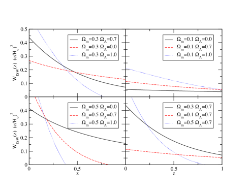
For the $\Lambda$CDM case the ISW effect is non-zero, and the kernel $W_{ISW}$ can be well approximated by $W_{ISW}(z)=-3\Omega_{m}(H_{0}/c)^{2}D(z)(f-1)$, where f is the relative growth factor, $f\simeq\Omega_{m}(z)^{6/11}$. $W_{ISW}$ decreases as a function of increasing redshift and goes to zero both for $\Omega_{m}\rightarrow 0$ and for $\Omega_{m}\rightarrow 1$. At low redshifts, the ISW effect is larger for larger values of $\Omega_{m}$, but the redshift evolution depends on the curvature (ie how quickly the $H$ and $D$ evolve to the EdS case). This is illustrated in Fig.1 which shows how $W_{ISW}$ depends on $z$ for different values of $\Omega_{\Lambda}$ and $\Omega_{m}$. At high redshifts, the lower the value of $\Omega_{\Lambda}$ (for a fixed $\Omega_{m}$) the larger the ISW amplitude.

Figure 1: Redshift dependence of $W_{ISW}(z)$ in Eq.[2.1] for different values of $\Omega_{m}$ and $\Omega_{\Lambda}$. Bottom left, top right and top left panels shows a fixed $\Omega_{m}=0.5$, $\Omega_{m}=0.3$ and $\Omega_{m}=0.1$ respectively. In all cases: $\Omega_{\Lambda}=0.0$ (dotted blue line) , $\Omega_{\Lambda}=0.7$ (continuos black line) and $\Omega_{\Lambda}=1.0$ (dashed red line). Bottom right panel shows a fixed $\Omega_{\Lambda}=0.7$ and $\Omega_{m}=0.3$ (continuos black line), $\Omega_{m}=0.5$ (dotted blue line) and $\Omega_{\Lambda}=0.1$ (dashed red line).

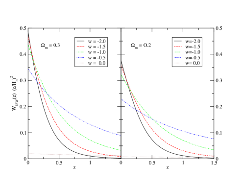
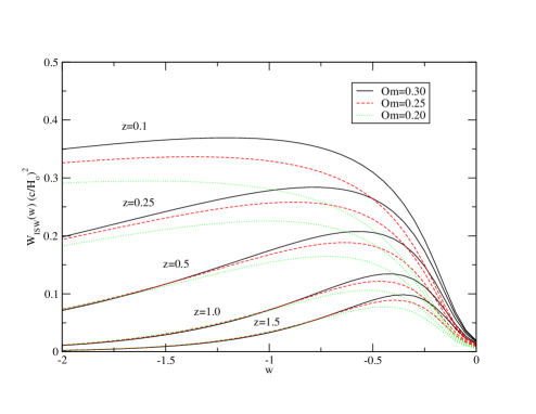
In Figures 2 and 3 we also shown for a given flat cosmology model the dependence of the $W_{ISW}$ on redshift and on the equation of state parameter w. For a given redshift and $\Omega_{m}$ there exists a maximum of $W_{ISW}$ around $w=-0.5$. This maximum would translate into a maximum in the cross-correlation signal $w_{TG}$. If data turns out to be greater than this maximum this would clearly disfavor models with constant equation of state.

Figure 2: Redshift dependence of $W_{ISW}$ in eq [2.1] for flat models with constant equation of state. Right panel shows a fixed $\Omega_{m}=0.2$ and left panel $\Omega_{m}=0.3$. In both cases $w=-2$ (black continuous line), $w=-1.5$ (red dashed line), $w=-1$ (green dot-dashed line), $w=-0.5$ (blue doubledot-dashed line), and $w=0$ (brown dotted line)

Figure 3: Dependence of $W_{ISW}$ on the equation of state parameter $w$ for flat models at different redshifts and values of $\Omega_{m}$. $\Omega=0.3$ (back continuous lines), $\Omega_{m}=0.25$ (red dashed lines), $\Omega_{m}=0.2$ (green dotted lines). Redshifts are 0.1, 0.25, 0.5, 1.0, 1.5 from top to bottom.

2.2 Bias Self-calibration

Linear bias is used to study how well light traces the underlying statistics of linear matter fluctuations. On these very large scales, fluctuations $\delta$ are small and linear theory works very well both for biasing and gravity. We remove the effects of biasing in our parameter estimation by comparing the observed galaxy-galaxy correlation $w_{GG}$, in the very same samples used for the cross-correlation, to the matter-matter correlation $w_{mm}$ predicted by each model (?). The effects of bias are also redshift dependent, but given a galaxy selection function $\phi_{G}(z)$, picked at $z=\bar{z}$, we approximate the bias with a constant $b=b(\bar{z})$ for that particular survey. We then have: $w_{TG}=b(\bar{z})w_{Tm}$ and $w_{GG}=b^{2}(\bar{z})w_{mm}$, so that an effective linear bias $b$ can be estimated as the square root of the ratio of galaxy-galaxy and matter-matter correlation functions:

$$b=\sqrt{{w_{GG}\over w_{mm}}}.$$ (9)

Such prescription has been shown to work well in a variety of galaxy models (eg see (?)). The values of $w_{mm}$ can be computed similar to (2.1) by

$$w_{mm}(\theta) = {1\over{2\pi}}\int dkkP(k)g(k\theta)$$

$$g(k\theta) = \int dz\,W_{m}^{2}(z){H(z)\over c}J_{0}(k\,r_{A}\theta)$$ (10)

$$W_{m}(z) = \phi_{G}(z)D(z),$$

where the only difference between $W_{m}$ and $W_{G}$ is the bias factor $b(z)$ in Eq.[2.1]. Note how the estimation of $b$ in Eq.[9] depends on the normalization of the power spectrum in $w_{mm}$. We choose to normalize each model by fixing $\sigma_{8}$. To make our results independent of this normalization we will marginalize over $\sigma_{8}$ and $h$. Taking flat priors and ranges $\sigma_{8}=0.8-1.0$ and $h=0.72-0.77$. We compare the predictions with the observational data $w_{TG}$ normalized to the CCM model bias, ie $w_{TG}/b$, where $b$ is estimated from Eq. (9) using $w_{mm}$ in the CCM model. Consequently, for other models, we will need to renormalize each of the theoretical predictions to the CCM model bias using a “relative bias”: $w_{TG}^{mod}/b=b_{r}\;w_{tm}^{mod}$, where $b_{r}^{2}={w_{mm}/w_{mm}^{mod}}$ is the ratio of the concordance model prediction to the one in the corresponding model. We choose to estimate this relative bias at $R=8$ Mpc/h, but the actual number has little effect in our final conclusions.

3 Observational Data

Recent analysis by independent collaborations, have cross-correlated the CMB anisotropies measured by WMAP with different galaxy surveys. The median galaxy redshifts expand over a decade (ie $0.1<\bar{z}<1.0$) and trace the matter distribution with light from the whole range of the electromagnetic spectrum: radio, far-infrared, optical and X-ray surveys (see Table 1). The cross-correlation and error estimation techniques used are also quite different but they yield comparable results over the scales of interest. Compare for example the Montecarlo errors to jackknife errors in Fig.3 in ?. In our compilation of the different data sets, we average the results on fixed angular scales around $\theta=6^{\circ}$. This corresponds to proper distances of $\simeq 25$Mpc/h at $\bar{z}\simeq 0.1$ and $\simeq 100$ Mpc/h at $\bar{z}\simeq 1.0$ in the CCM model and avoids possible contamination from the small scale SZ and lensing effects, eg see Fig. 3 in ?.

Radio galaxies from NVSS (?) and hard X-ray background observed by HEAO-1 (?), have been cross-correlated with WMAP data (?; ?), to find a signal of $1.13\pm 0.35\,$ times the CCM model prediction at $z\sim 0.9$. The different biases for X-rays, $b^{2}=1.12$, (?) and for radio galaxies, $b=1.3-1.7$, (?) have been taken into account. A compatible signal has also been found with the NVSS data by the WMAP team (?).

The cross correlation of WMAP with galaxies ($17<b_{J}<20$) in the APM Galaxy Survey (?) (covering about 20% of the South Galactic Cap, SGC) was found to be $w_{TG}=0.35\pm 0.13\,\mu K$ at scales $\theta=4-10^{\circ}$ with $b\simeq 1$ (?). The cross-correlation of WMAP with the SDSS DR1 (?) (covering about 10% of the North Galactic Cap, NGC) have been done for several subsamples (?). The first sample ($\bar{z}\sim 0.3$) contains $\sim 5$ million objects classified as galaxies in SDSS (with $r<21$ and low associated error). For this sample, which has $b\simeq 1$, $w_{TG}=0.26\pm 0.13\,\mu K$ at scales $\theta=4-10^{\circ}$. The high redshift sample ($z\sim 0.5$) has $w_{TG}=0.53\pm 0.21\,\mu K$ and $b^{2}\simeq 6$. The SDSS data has also been cross-correlated with WMAP by the SDSS team (?) using nearly 25 million galaxies in four redshift samples. Their results are similar with those obtained earlier by ? but no bias from galaxy-galaxy auto correlation function is given. The infrared 2MASS Galaxy Survey (?), with $z\sim 0.1$, show a WMAP cross-correlation of $1.53\pm 0.61$ times the CCM prediction, with a bias of $b=1.18$ (?).

We have selected independent measurements for which the bias CCM $b$ (from $w_{GG}$) is known, so that we can applied the bias “self-calibration” proposed in section §2.2. The data is summarized in Table 1 and displayed in Fig.1. In the results below we also include a $10\%$ uncertainty in the median redshift. We chose the values of NVSS+HEAO-1 quoted by (?) as representative of both the ? and ? analysis. For the SDSS, we chose the values in ? where the CCM bias $b$ is estimated using Eq.(9). Note how the selected samples are complementary. The samples which have large sky overlap (eg 2MASS and NVSS+HEAO-1) have negligible redshift overlap. When the redshift overlap is significant (ie in 2MASS-APM or SDSS-NVSS could be up to $20\%$) the sky overlap is small (less than $10\%$). Consequently, the different samples in Table 1 have less than $1\%$ volume in common. This is negligible, given that individual sampling errors (which are proportional to volume) are of the order of 30%.

The most significant detection in Table 1 seems to be the one quoted by ? for the NVSS+HEAO-1 samples. Given the systematic uncertainties involved in the bias and selection function of both of these samples, we have checked that our results do not changed much (less than $20\%$ in the area of the contours in Fig.3) when we double the quoted errorbar. Doubling this errorbar corresponds to an additional $50\%$ systematic uncertainty in the value $b$ or to a $40\%$ uncertainty in the median redshift of the samples.

The observational data not included in Table 1 is in good agreement with the values in the table, but is excluded to avoid redundancy. The agreement of the redundant data provides further confirmation and indicates that errors are dominated by sampling variance rather than by the methodology or the systematics.

$\bar{z}$	$w_{TG}/b$	$b$	catalog, Band
0.1	$0.70\pm 0.32$	1.1	2MASS, infrared ($2\mu m$)
0.15	$0.35\pm 0.17$	1.0	APM, optical ($b_{j}$)
0.3	$0.26\pm 0.14$	1.0	SDSS, optical ($r$)
0.5	$0.216\pm 0.096$	2.4	SDSS high-z, optical ($r$+colors)
0.9	$0.043\pm 0.015$	1-2	NVSS+HEAO, Radio & X-rays

Table 1: Observed cross correlation $w_{TG}/b$ (averaged for $\theta\simeq 4-10^{\circ}$.) of WMAP anisotropies with different catalogs. Errors in $w_{TG}/b$ includes 20% uncertainty in $b$. Errors in the median redshift $\bar{z}$ are about 10% .

Figure 4: Symbols with error bars correspond to the different measurements $w_{TG}/b$ in Table 1. As an illustration of the shape, the continuous, short-dashed and long-dashed lines show the concordance ($\Omega_{m}=0.3,\Omega_{\Lambda}=0.7$), opened ($\Omega_{m}=0.3,\Omega_{\Lambda}=0.0$) and closed ($\Omega_{m}=0.3,\Omega_{\Lambda}=1.1$) model predictions (at $\theta=6^{\circ}$). The dotted line corresponds to the galaxy-galaxy prediction (and also the dust contamination model). All lines have arbitrary normalization.

4 Results

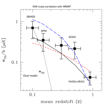
Fig.4 compares the $w_{TG}$ observations with predictions for a fixed value of $\Omega_{m}=0.3$ and three different values of $\Omega_{\Lambda}$. We can see how the shape of the prediction depends on the amount of dark energy. Even though $W_{ISW}$ at $z=0$ depends only weakly on $\Omega_{\Lambda}$, the evolution with redshift depends more strongly on $\Omega_{\Lambda}$. For a fixed $\Omega_{m}$, models with larger values of $\Omega_{\Lambda}$ evolve more rapidly with redshift to the EdS case, where the ISW effect vanishes. Thus, contrary to what happens at $z=0$, the lower the value of $\Omega_{\Lambda}$ (for a fixed $\Omega_{m}$) the larger the ISW amplitude at high redshifts (see also Fig.1).

To test model predictions with the data, we use a standard $\chi^{2}$-test, $\chi^{2}=\sum_{i}~{}(O_{i}-T_{i})^{2}/\sigma_{i}^{2}$, where $O_{i}$ and $\sigma_{i}$ correspond to the different measurements and errors and $T_{i}$ correspond to the model. The label $i$ runs for $i=1$ to $i=5$ marking the different data points (column 1 in Table 1) as we move in redshift. In order to take into account the error in the median redshift we take:

$$\sigma_{i}^{2}=\sigma_{w}^{2}+\left({{d(w_{tg}/b)}\over{dz}}\right)^{2}\;\sigma_{z}^{2}$$ (11)

where $\sigma_{z}$ and $\sigma_{w}$ are the errors in the $w_{TG}/b$ and $\bar{z}$ respectively (see Table 1). We use the relative $\chi^{2}$ values, $\chi^{2}-\chi^{2}_{min}$, to define confidence levels in parameter estimation. Top panel of Fig.5 shows the resulting confidence contours. Taking $T_{i}=0$ we evaluate the significance of the combined ISW detection. We find that this null hypothesis is rejected with a very high probability: $P\simeq 99.997\%$ (from $P_{\nu=4}(\chi^{2}>26)\simeq 3\times 10^{-5}$). We next compute the expected ISW effect and compare it with the observational data within the $\Lambda$CDM family of models, where $\Omega_{m}$, $\Omega_{\Lambda}$ and $h$ are free parameters (we fix the baryonic content $\Omega_{b}\simeq 0.05$ and the primordial spectral index $n_{s}\simeq 1$). We choose to normalize each model by fixing $\sigma_{8}$. To make our results independent of this normalization we will marginalize $\sigma_{8}$ over the range $\sigma_{8}=0.8-1.0$ (flat prior used). As we compare $w_{GT}$ normalized to the CCM model bias, we need to compute the relative bias for other LCDM models (see section §2.2). We choose to estimate this at $R=8Mpc/h$, but the actual number has little effect in the conclusions. We have also marginalized over $h$ in a flat prior range $h=0.72-0.77)$. Our results are not very sensitive to the ranges used for $\sigma_{8}$ and $h$: increasing these ranges by a factor of two change our contours in less than 20 %.

Figure 5: One, two and three sigma confidence contours in the $(\Omega_{m},\Omega_{\Lambda})$ plane (marginalized over $h$) for the $\Lambda$CDM model. Top: constraints from only ISW. Bottom: constraints from SNIa (blue) and ISW (green) along with the combined contours (purple).

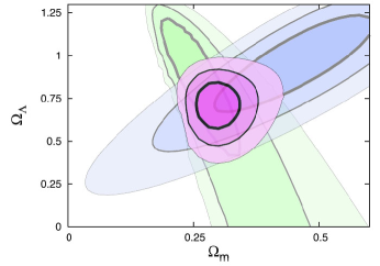
The best fit using only ISW data corresponds to $\Omega_{m}\simeq 0.26\pm 0.08$, $\Omega_{\Lambda}\simeq 0.82\pm 0.40$, in good agreement with other cosmological probes mentioned above. Bottom panel of Fig. refcombinedconts we show the confidence contours for a $\Lambda$CDM model along with the constraints from recent SNIA (?) observations. From the figure it is clear how the ISW effects gives new complementary information about the cosmological parameters. The EdS model is ruled out to high significance. The confidence contours are almost perpendicular to the SNIA contours, allowing to constrain the parameter space of the model well with just these two observations. Combination of ISW with supernova data yields $\Omega_{\Lambda}=0.71\pm 0.13$ and $\Omega_{m}=0.29\pm 0.04$.

4.1 Uncertainties in the selection function

We explore here how robust are our results to the uncertainties in the galaxy selection function. We take a generic parametric form of the type:

$$\phi(z)dz={1\over\Gamma({m+1\over\beta})}\beta{z^{m}\over z_{0}^{m+1}}e^{\left(-{z\over z_{0}}\right)^{\beta}}dz$$ (12)

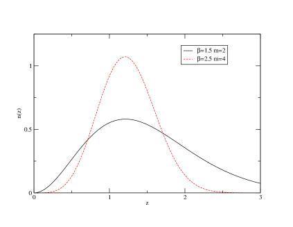
so that it is normalized to unity. Parameters $\beta$ and $m$ control the shape of the function and are treat as fix parameters; $z_{0}$ is being changed accordingly to the median redshift $\bar{z}$ we want for the selection function. When computing our results we use $\beta=1.5$ and $m=2$, in which case $\bar{z}=1.41{z_{0}}$.

In order to clarify the role of the selection function shape we recalculate our results with a much more peaked selection function. This second selection function have $\beta=2.5$ and $m=4$ and it is plotted together with the fiducial one in Figure 6. Both cases have the same median redshift $\bar{z}=1.41$. Top panel of Fig.7 shows the contours in the $(\Omega_{m},\Omega_{\Lambda})$ plane for the more peaked selection function (with $\beta=2.5$ and $m=4$). The contours are similar to the fiducial model (ie compare to Fig. 5) but favoring slightly lower values for $\Omega_{\Lambda}$ and $\Omega_{m}$.

Figure 6: Two different selection functions with the same median redshift $\bar{z}=1.41$. Both have the generic form given by the equation [12]. The black continuous line corresponds to $\beta=1.5$ and $m=2$ while the red dashed line is for $\beta=2.5$,$m=4$

Besides the uncertainty on the shape of the selection function  there is also uncertainty in the median redshift. We have checked what happens if this uncertainty is not taken into account. We just set the redshift errors $\sigma_{z}=0$ in Eq.[11]. Contours for the $(\Omega_{m},\Omega_{\Lambda})$ plane are plot in the bottom panel of figure 7, which are also to compare with figure 5. There is hardly any difference because the theoretical values of $w_{TG}$ change very little within the median redshift error range.

Figure 7: One, two and three sigma confidence contours in the $(\Omega_{m},\Omega_{\Lambda})$ plane for the $\Lambda$CDM model. Top panel: contours using a more peaked selection function ($\beta=2.5$, $m=4$) but with the same mean redshift as the fiducial case (ie compare to Fig.5). Bottom panel: contours when errors in the median redshift of the selection functions are neglected.

4.2 Equation of state

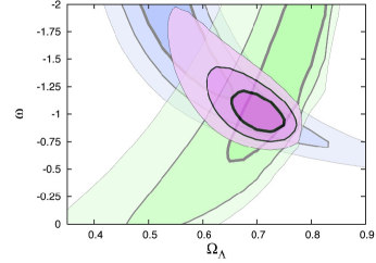
The ISW effect can also be used to constrain the dark energy equation of state parameter. In this case, as suggested by the CCM, we assumed a flat universe. We focus on a constant $w$ parameter and maintain the same flat priors for $h$ and $\sigma_{8}$ ( $0.72<h<0.77\;\;0.8<\sigma_{8}<1.0$ ). Top panel of Figure 8 show the one,two and three sigma contours for the ($\Omega_{m},w$) plane using only the ISW data. Join contours with the SNIa data are shown in the bottom panel of Figure 8. Both datasets are also complementary for the $w$ determination. The SNIa data is from (?).

Making a join ISW+SNIa analysis with the flat prior reduces notably the allowed space for the parameters to $w=-1.02\pm 0.17$ and $\Omega_{\Lambda}=0.70\pm 0.05$. The contours are comparable with other analysis in literature (?) which combines SNIa with WMAP and SDSS data. The results we found are still in full agreement to the CCM with $\Omega_{\Lambda}\simeq 0.7$ and $w=-1$.

Figure 8: One, two and three sigma confidence contours in the $(\Omega_{\Lambda},w)$ plane (marginalized over $h$ and $\sigma_{8}$. Top: constraints only from ISWfrom ISW. Bottom: constraints from SNIa (blue) and ISW (green) along with the combination (purple).

4.3 Possible Contaminants

The constraining power of the new ISW data comes from the simultaneous fitting of data at different redshifts, that is from the shape information in Fig. 4. Because of the uncertainties in the relative normalization due to a relative bias, any given point alone does not constrain well the cosmological parameters. But the combination of the data gives us a new powerful tool for cosmological parameter estimation.

The shape of the curve as a function of redshift also provides an important test for systematics. CMB and galaxy maps are both masked and corrected from galactic absorption/extinction, but any residual contamination could produce a cross-correlation signal. Emission and absorption by our own galaxy produce patchy hot spots in the CMB maps and negative density fluctuations in the galaxy distribution (because of extinction). In principle, this should therefore result in a negative cross-correlation, but overcorrecting for the effects of galactic absorption could also result in a positive signal. This possibility have been tested for each of the samples, by comparing the cross-correlation to WMAP maps at different frequencies. Most analysis use the WMAP Kp0 mask, which excludes about $30\%$ of sky on the basis of galactic or extra-galactic (eg radio sources) contamination. In all cases the contamination seems smaller than the errors (eg see Fig. 2 in ?). Moreover, one does not expect this effect to have any redshift dependence, contrary to the measurements in Fig. 4.

Cold dust in distant galaxies, will also produce patchy hot spots in the CMB maps and positive density fluctuations in the galaxy distribution (could also be negative because of internal extinction). The resulting cross-correlation should trace the galaxy-galaxy auto correlation function, $w_{GG}$, and should therefore have a very different redshift dependence to the ISW effect. The dotted line in Fig. 4 shows the predicted shape dependence for $w_{GG}$ contamination with arbitrary normalization. The shape is clearly incompatible with the actual cross-correlation measurements. It is also worth noting how $w_{GG}$ goes quickly to zero at $\bar{z}\simeq 0.2$, while the ISW cross-correlation remains positive. This is due to the fact that at these corresponding large scales, $\;\raise 1.29167pt\hbox{$>$\kern-7.5pt\raise-4.73611pt\hbox{$\sim$}}\;40$ Mpc/h, matter-matter correlations $w_{mm}$ effectively decays to zero, while $w_{TG}$, which traces the gravitational potential, has a less rapid decay with distance.

5 Conclusion

The cross-correlation of CMB anisotropies with very different galaxy surveys provides consistent detections. Their combination follows the CCM predictions with a probability of only $\simeq 3\times 10^{-5}$ for being a false detection. This provides new and independent evidence for dark energy and dark matter, ruling out the EdS model to a high significance (for any value of $H_{0}$). Combination with SNIA data results in strong constraints to $\Omega_{\Lambda}=0.71\pm 0.13$ and $\Omega_{m}=0.29\pm 0.04$. This in good agreement with the flat universe $\Omega_{m}+\Omega_{\Lambda}\simeq 1$ found independently by CMB data (?; ?). If we assume a flat universe, we find $\Omega_{\Lambda}=0.70\pm 0.05$ and $w=-1.02\pm 0.17$ for a constant dark energy equation of state. The data shows, for the first time, statistical evidence of a recent slow down in the growth of structure formation on linear scales, just as expected in a flat accelerated universe. The new ISW constraints rely in a totally different physical effect that previous cosmological constraints, providing new light on a dark cosmos.

Note added in proof: After this paper was originally submitted to astro-ph (astro-ph/0407022) a related analysis using our data compilation have been published by Corasanniti, Giannantonio and Melchiorri (astro-ph/0504115).

References

- [Afshordi, Loh & Strauss ¡2004¿] Afshordi, N. , Loh, Y., Strauss, M. A., 2004, Phys. Rev. D 69, 083524
- [Afshordi ¡2004¿] Afshordi,N., 2004 astro-ph/0401166.
- [Barriga etal ¡2001¿] Barriga, J., Gaztañaga, E.,Santos, M.G., Sarkar,S., 2001, MNRAS 324, 977
- [Barris et al. ¡2004¿] Barris, B. J. et al., 2004, ApJ 602, 571.
- [Bennett et al. ¡2003¿] Bennett C.L. et al., 2003, ApJ Suppl., 148,1
- [Berlind, Naratanan & Weinberg ¡2001¿] Berlind, A., Naratanan, V., Weinberg, D., 2001, ApJ 549, 688
- [Blanchard ¡2003¿] Blanchard, A., Douspis, M., Rowan-Robinson, M., Sarkar, S., 2003, A&A, 412, 35.
- [Boldt ¡1987¿] Boldt, E., 1987, Phys. Rep. 146, 215.
- [Boughn & Crittenden ¡2004a¿] Boughn, S., Crittenden, R. 2004, Nature 427, 45
- [Boughn & Crittenden ¡2004b¿] Boughn, S., Crittenden, R. 2004, astro-ph/0404470
- [Boughn & Crittenden ¡2003¿] Boughn, S., Crittenden, R. 2003, astro-ph/0305001
- [Boughn & Crittenden ¡2002¿] Boughn, S., Crittenden, R. 2002, Phys. Rev. Lett. 88, 021302
- [Condon etal ¡1998¿] Condon J. J. et al., 1998, AJ 115, 1693
- [Crittenden & Turok ¡1996¿] Crittenden, R. G. Turok, N., 1996, Phys. Rev. Lett. 76, 575.
- [Einseintein & Hu ¡1999¿] D.J. Einseinstein & W. Hu, 1998, Astrophys. J. 496, 605
- [Fosalba & Gaztañaga ¡2004¿] Fosalba, P. Gaztañaga, E., 2004, MNRAS 350, 37
- [Fosalba, Gaztañaga & Castander ¡2003¿] Fosalba, P. Gaztañaga, E., Castander, F.J., 2003, ApJ 597, L89
- [Gaztañaga & Baugh ¡1998¿] Gaztañaga,E. & Baugh, C. M., 1998, MNRAS, 294, 229
- [Gaztañaga & Lobo ¡2001¿] Gaztañaga, E., & Lobo, J. A., 2001, ApJ 548, 47
- [Jarret et al. ¡2000¿] Jarret, T. H., et al., 2000, AJ 119, 2498
- [Lue & Starkman ¡2004¿] Lue, A., Scoccimarro, R., Starkman, G., 2004, Phys. Rev. D, 69, 044005
- [Maddox et al. ¡1990¿] Maddox, S. J. ,Efstathiou, G., Sutherland, W. J., Loveday, J., 1990, MNRAS 242, 43P
- [Multamäki, Gaztañaga & Manera ¡2003¿] Multamäki, T., Gaztañaga, R., Manera, M., 2003, MNRAS 334, 761
- [Nolta et al. ¡2004¿] Nolta, M. R. et al. 2004, ApJ 608, 10
- [Peacock et al. ¡2001¿] Peacock, J. A. et al., 2001, Nature, 410, 169
- [Percival et al. ¡2001¿] Percival W.J. et al., 2001, MNRAS, 327, 1297
- [Perlmutter et al. ¡1999¿] Perlmutter, S. et al., 1999, ApJ 517, 565
- [Pope et al. ¡2004¿] Pope, A. C. et al., 2004, ApJ, 607, 655
- [Riess et al. ¡1998¿] Riess A. G. et al., 1998, AJ 116, 1009
- [Sachs & Wolfe ¡1967¿] Sachs,R. K., Wolfe, A. M., 1967, ApJ 469, 437
- [Sandvik et al ¡2004¿] Sandvik H.B., Tegmark M., Wang X., andZaldarriaga M., Phys. Rev. D69, 063005
- [Scranton et al. ¡2003¿] Scranton, R. et al., 2003 astro-ph/0307335.
- [Tegmark et al. ¡2004¿] Tegmark, M. et al., 2004, ApJ, 606, 70