Empirical Modeling of the Stellar Spectrum of Galaxies

Abstract

An empirical method of modeling the stellar spectrum of galaxies is proposed, based on two successive applications of Principal Component Analysis (PCA). PCA is first applied to the newly available stellar library STELIB, supplemented by the J, H and K_s magnitudes taken mainly from the 2 Micron All Sky Survey (2MASS). Next the resultant eigen-spectra are used to fit the observed spectra of a sample of 1016 galaxies selected from the Sloan Digital Sky Survey Data Release One (SDSS DR1). PCA is again applied, to the fitted spectra to construct the eigen-spectra of galaxies with zero velocity dispersion. The first 9 galactic eigen-spectra so obtained are then used to model the stellar spectrum of the galaxies in SDSS DR1, and synchronously to estimate the stellar velocity dispersion, the spectral type, the near-infrared SED, and the average reddening. Extensive tests show that the spectra of different type galaxies can be modeled quite accurately using these eigen-spectra. The method can yield stellar velocity dispersion with accuracies better than 10%, for the spectra of typical S/N ratios in SDSS DR1.

1 INTRODUCTION

The observed spectrum of a galaxy is a combination of three components: a continuum, absorption lines and emission lines. For non-active galaxies, the continuum and the absorption line components in the optical and near-infrared are usually dominated by starlight, while in the mid/far-infrared they are dominated by dust and hot gas emission. For active galaxies, the continuum is diluted by the featureless continuum of the nucleus. For active and non-active galaxies, the continuum is modified to varying degrees by reddening. The emission line component is produced in H ii regions around hot stars or in the emission line regions of the active nucleus. A proper decomposition of the emission line component on one hand and the continuum plus absorption line component (so called the stellar spectrum) on the other is the first step toward a physical interpretation of the spectrum. For instance, accurate measurement of emission lines is fundamental to the identification and classification of AGN. However, the optical spectra of many nuclei are heavily contaminated, even dominated, by stellar absorption lines coming from the host galaxy. Therefore, it is imperative that the underlying starlight be properly removed before the AGN identification. As for studying nebular emission lines and the abundances of gaseous material, proper starlight removal is also necessary. Moreover, a well-modeled stellar spectrum may provide direct information on the stellar population, accurate measurement of the stellar velocity dispersion, and hence some fundamental properties of the host galaxy, such as spectral type, kinematics, star formation history, etc.

Though various schemes have been proposed to subtract the underlying starlight, the basic procedure is quite similar: a library of absorption-line templates are built in the first place, either from spectra of stars or from that of pure absorption-line galaxies; secondly the templates are used to model the non-emission-line region of the spectrum; at last the modeled spectrum, which is taken as the integrated spectrum of the stellar component, is removed.

When spectra of stars are employed to construct the templates, the most common approach is stellar population synthesis. There are two main types of population synthesis studies: evolutionary population synthesis (Tinsley 1967; Bruzual & Charlot 2003) and empirical population synthesis (Faber 1972; Kong et al. 2003). For the former, the age- and metallicity-dependent models of stellar spectra are developed by assuming the time evolution of a few main parameters, and then used to reconstruct the integrated spectrum of stellar systems. However, modern evolutionary population synthesis models still suffer from serious uncertainties, which appear to originate from the underlying stellar evolution theory, the color-temperature scale of giant stars, and, for non-solar abundances in particular, the flux libraries (Charlot, Worthey & Bressan 1996). The empirical population synthesis approach reproduces the stellar spectrum with a linear combination of the spectra of a library of stars or star clusters. Compared to the evolutionary population synthesis, the merit of this approach is that the result does not depend on any assumed parameters, while the drawback is its strong dependence on the coverage range of metallicity, spectral type and luminosity class of the stellar library. Another drawback is that this approach can not predict the past and future stellar properties of galaxies.

When spectra of galaxies are used, the templates are usually derived either from the spectrum of another galaxy with no/weak emission lines, or from that of an off-nuclear position in the same galaxy (Ho, Filippenko & Sargent 1997, and references therein). However, the spectrum of another galaxy may not accurately reflect the exact stellar content of the galaxy being studied, while the off-nuclear spectrum may not be completely free of line emission. Instead of using a single galactic spectrum as the template, which is often chosen subjectively, Ho, Fillipenkko & Sargent (1997) used an objective algorithm to find the best combination of galactic spectra to create an ”effective” template. The advantage of this modification is that the use of a large basis of input spectra ensures a closer match to the true underlying stellar population. Recently, Hao et al. (2002) applied Principal Component Analysis (PCA, Deeming 1964) to several hundred pure absorption-line galaxies and used the first few eigen-spectra as the templates. This makes the size of the template library much smaller because the most prominent features from the sample concentrate into the first few eigen-spectra. The other merit is that the best-fitting model is unique because the eigen-spectra are orthogonal. However, both of the above methods have their unavoidable shortcomings. Because the templates are derived from the observed spectra of galaxies, in which the stellar velocity dispersion is non-zero and varies from object to object, they usually do not match the velocity dispersion of the galaxies in question. Furthermore, the template library consists of only pure absorption-line galaxies, which usually contain very little or no young stellar component. As a result, the modeled spectra could not reflect correct information on the stellar population of emission-line galaxies, giving rise to inaccurate representative spectra.

We present here a robust and efficient method of starlight removal in the optical and the near-infrared band. Briefly, PCA is first applied to the optical spectra of STELIB (Le Borgne et al. 2003), a newly available stellar library in the wavelength coverage of 3500–9500Å, and the near-infrared photometric data at J, H, and K_s bands collected from the 2 Micron All Sky Survey (2MASS; Skrutskie et al. 1997), supplemented by the stellar library presented by Pickles (1998) (§3). The stellar eigen-spectra in the visible range are then used to model a homogeneous library of 1016 galactic spectra picked up from the Sloan Digital Sky Survey Data Release One (SDSS DR1; Abazajian et al. 2003). PCA is again applied to the modeled galactic spectra with zero stellar velocity dispersion. The first 9 eigen-spectra are selected as the final absorption-line templates (§4). Using these templates, the stellar spectrum of the galaxies in SDSS DR1 can be well modeled and the stellar velocity dispersion, the near-infrared SED, the spectral type and the average reddening of galaxies can be obtained simultaneously (§5). Extensive tests show that the present method is self-consistent and robust.

2 PRINCIPAL COMPONENT ANALYSIS

The purpose of this section is to summarize briefly the PCA method and provide the definition of terms used in this paper.

PCA is a method used to reveal interrelations among different variables and objects contained in a large, multivariate dataset. Its aim is to reduce the number of dimensions in the data space, so that the most important information can be extracted. Let the sample being studied be a collection of $n$ objects, for each of which there are $m$ observational variables. So one have a matrix ${\bf X}=\{x_{ij}\}_{n\times m}$ ($i=1,\cdots,n$ and $j=1,\cdots,m$), each row vector of which corresponds to the different variables of a given object, while each column vector, to the same variable of the various objects. PCA proceeds from the given matrix ${\bf X}$ and yields $m$ new variables, the principal components (PCs), which are mutually independent and generally, the first $m^{\prime}$ ($m^{\prime}\ll m$) PCs contain a majority of the information of the data. Each PC is a linear combination of the original $m$ variables; the corresponding coefficient vector is called eigenvector. Furthermore, via the eigenvectors, the original $m$ variables of each object are projected onto the PCs to yield the new variables of this object. For example, the $j$-th PC of $i$-th object is given by

$$pc_{ij}={\rm\mathbf{e_{j}}}\cdot{\rm\mathbf{x_{i}}}=e_{j1}x_{i1}+\cdots+e_{jk}x_{ik}+\cdots+e_{jm}x_{im}\,,$$ (1)

where $\rm\mathbf{x_{i}}$ is the $i$-th row vector of $\mathbf{X}$, and $\rm\mathbf{e_{j}}$ is the eigenvector of the $j$-th principal component.

The fundamental principles of PCA could be understood as follows. The contribution of PCs to the variance of the original dataset is a measure of the amount of original information contained in the PCs. Thus, the destination of PCA method is to seek the set of eigenvectors that give rise to PCs with the maximum variance. According to the theory of statistics, the expected eigenvectors are essentially the orthogonal eigenvectors of the covariance matrix ${\bf C}=\{c_{jk}\}_{m\times m}$, where

$$c_{jk}=\frac{1}{n-1}\sum_{i=1}^{n}(x_{ij}-\bar{x_{j}})(x_{ik}-\bar{x_{k}})\,;\hskip 17.07164pt1\leq j\,,k\leq m\,.$$ (2)

Accordingly, the covariance matrix ${\bf C}$ is first constructed. Then the determinant equation $|{\bf C}-l{\bf I}|=0$ is solved to find the $m$ eigenvalues $\{l_{j}\}$ ($l_{1}\geq l_{2}\geq l_{3}\geq...\geq l_{m}\geq 0$), where ${\bf I}$ is the unit $m\times m$ matrix. After this, by solving the equation $({\bf C}-l_{j}{\bf I}){\bf e_{j}}=0$, the eigenvectors ${\bf e_{j}}$ are obtained. Since there are $m$ eigenvalues, there will be at most $m$ eigenvectors. The PCs are ordered by decreasing the eigenvalues, which are generally used to characterize the contribution of the corresponding principal components to the original information. The quantity $l_{j}/\sum\limits_{i=1}^{m}l_{i}$ is called the fractional or relative contribution of the $j$-th principal component, and $\sum\limits_{j=1}^{k}l_{j}/\sum\limits_{j=1}^{m}l_{j}$, the cumulative contribution of the first $k$ principal components. In general, it is not necessary to find all the $m$ principal components: most of the information is contained in the first few, with the first one having the lion’s share.

Much has been written about the use of PCA in studies of the multivariate distribution of astronomical data (Connolly et al. 1995, and reference therein). In most of earlier studies, the variables of the original dataset are observed (generally normalized) fluxes at $m$ wavelength channels of $n$ celestial bodies (objects), giving a matrix of ${\bf X}=\{x_{ij}\}_{n\times m}$; the resultant $m$ eigenvectors with $m$ wavelength channels for each eigenvector are so called eigen-spectra, and used for further applications: spectral classification, modeling of stellar spectra, etc. In this paper, we perform PCA in a slightly different way: the input data matrix is transposed to be ${\bf X}=\{x_{ij}\}_{m\times n}$ before being analyzed, i.e. the variables now become the fluxes of various celestial bodies at given wavelength channel, and the objects are thus all the wavelength channels. In this case, PCA carries out an $n\times n$ matrix of eigenvectors, corresponding at most $n$ principal components. Thus, the projection of the $n$ celestial bodies onto the principal components gives rise to $n$ new spectra, which denotes $n$ ”new” celestial bodies, called ”eigen-star” or ”eigen-galaxy”. We then use these spectra as our templates for modeling.

The main difference between the above methods is easy be to understood. In the former case, the eigenvectors (eigen-spectra) correlate strongly with the prominent features present in the spectra of celestial bodies; thus the projection of a celestial spectrum onto a principal component gives a measure of the relative contribution of this celestial spectrum to the corresponding eigen-spectrum. However, in the latter, it is the eigenvectors that represent the contributions of the celestial bodies to the eien-stars or eigen-galaxies, while the spectra of the eigen-stars or eigen-galaxies contain various spectral features presented in original celestial spectra. We argue that, in some sense, the matrix-transposed method is much more effective and convenient. It is well known that a significant drawback of implementing PCA on large or very high-dimensional data sets is the required computation time (Madgwick et al. 2003). For $n$ spectra, each with $m$ wavelengths, this requires $O(nm^{2})$ operations. Therefore, if the data matrix is transposed, the operation will become $O(mn^{2})$, which is much smaller in the case of $m\gg n$. Given that each spectrum contains $O(10^{3})$ wavelength channels and the number of spectra is $O(10^{2})$, the latter method would reduce the computing expense by a magnitude. It goes without saying for analyzing spectra of higher resolution.

For convenience, the spectra of eigen-stars or eigen-galaxies, i.e the projection of the spectra of stars or galaxies onto principal components, are still called eigen-spectra in the following text, though its meaning is different from that in general case.

3 DERIVATION OF STELLAR EIGEN-SPECTRA

The stellar library is the foundation of applying the present method. It is conceivable that the quality of fits to observed galaxy spectra seriously hinges on the resolution of the stellar spectra, as well as the coverage of spectral type, luminosity class, chemical abundance, and wavelength range.

Theoretical stellar spectra are often preferred for spectral modeling, because of their uniformity and generally more extensive coverage (e.g Kurucz 1992; Lejeune 1997,1998; Westera et al. 2002). However, at the time of writing, no such library at the spectral resolution similar to/higher than that of SDSS spectra is available. Furthermore, these libraries may be biased in color and line strength, as many minor contributors to stellar opacity and to the emergent spectrum usually cannot all be included for the full spectral range because of computational constraints (Pickles 1998).

Several observed stellar libraries have been published, covering the ultraviolet (Heck et al. 1984; Robert et al. 1993; Walborn et al. 1995), optical(Gunn & Stryker 1983; Jacoby, Hunter & Christian 1984; Pickles 1985; Kiehling 1987), and near-infrared(Danks & Dennefeld 1994; Serote, Boisson & Joly 1996) wavelength ranges. They are usually obtained with different instrumentation, at different resolution, spectral sampling and for different purposes (Pickles 1998). The most common used stellar library is HILIB, presented by Pickles (1998), which consists of 131 flux-calibrated spectra with complete wavelength range from 1150 to 10620 Å in steps of 5 Å. However, the metallicity coverage of this library is limited to be near solar abundance, and the spectral resolution is relatively lower for accurately spectral modeling.

High resolution libraries spanning a wide range in metallicity, spectral type and luminosity class have only recently become available. The STELIB library (Le Borgne et al. 2003), a new spectroscopic stellar library, consists of an homogeneous library of over 250 stellar spectra covering the wavelength range from 3200 to 9500 Å, with a resolution of $\lesssim$ 3 Å (1Å sampling) and a signal-to-noise ratio of $\sim$ 50. The library includes stars of a range of metallicity from 0.05 to 2.5 times solar, a range of spectral type from O5 to M6 and luminosity class from I to V. Because of its wide coverage of spectral resolution and spectral type, this library represents a substantial improvement over previous stellar libraries (Le Borgne et al. 2003).

Although the visible region is always favored, the near-infrared is equally important because it reveals stars that remain hidden in the visible by interstellar dust (Combes et al. 2002). To extend the library into near-infrared band, we extract the infrared photometric data from 2MASS, which has mapped the full sky at three near-infrared wavelengths with 10 $\sigma$ sensitivity limits of J=15.8, H=15.1, and $K_{s}$=14.3 mag.

We therefore use STELIB as our star library. The optical spectra in STELIB and the corresponding near-infrared photometric data in 2MASS supplemented with HILIB are incorporated to form a star library of highest quality to date.

3.1 Optical Data

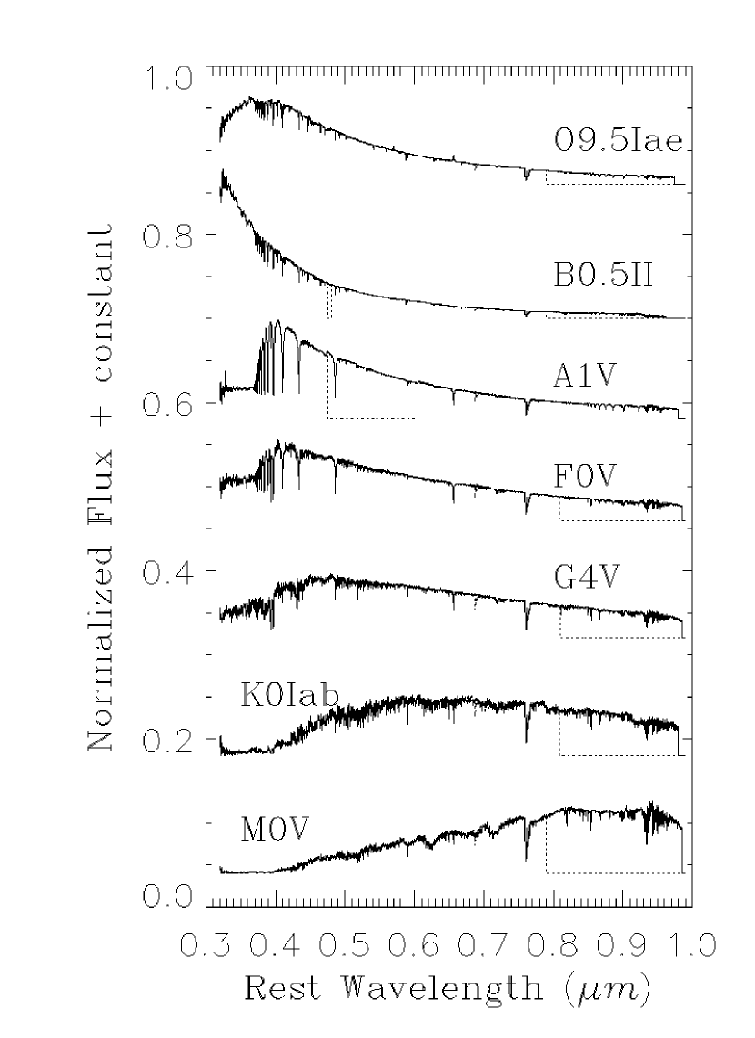
Figure 1: Examples of the filled spectra. The dashed lines represent the initial spectra in STELIB; the solid are the corresponding filled ones. Arbitrary constants were added to the scaled spectra for clarity.

The current public version of the STELIB library contains 255 optical spectra, which had been corrected for interstellar extinction and radial velocity. However, the data are missing in some limited wavelength range for nearly half of the stars. We use similar stellar spectra either from STELIB itself or from SDSS DR1 to fill the gaps of these spectra. Some examples of the result of this procedure are shown in Fig. 1 and at last 204 spectra are yielded.

Although about 50 spectra that could not be satisfactorily filled were ignored, the resultant stellar library is still homogeneous enough. The distributions of spectral types of the initial 255 stars and that of the final 204 stars are showed in Fig. 2. It is apparent that the coverage of spectral type of the resultant library is almost as good as that of the original.

There is no denying that, over previous stellar libraries, substantially improved as STELIB is, it still leaves much to be desired. As can be seen from Fig. 2, there are obviously two blank regions: early O, and late K, M and L types. The absence of these types of stars may have some influence on modeling the stellar spectrum of galaxies, especially for those mainly consisting of late-type stars.

3.2 Near-Infrared Data

We search for counterparts of the 204 stars in the 2MASS Pointed Source Catalog. Out of them, 182 have been detected in 2MASS. The magnitudes of these stars at J (1.235$\pm$0.006 $\mu m$), H (1.662$\pm$0.009 $\mu m$) and K_s (2.159$\pm$0.011 $\mu m$) bands are then transferred to fluxes $f_{J}$, $f_{H}$ and $f_{K}$ in unit of erg$\cdot$s^-1cm^-2Å^-1, according to the following formulas (see Mannucci et al. 2001),

$$\begin{array}[]{lll}f_{J}=3.129\times 10^{-0.4(J+25.0)}&,&\Delta f_{J}=(0.0175-0.4\Delta J)\cdot f_{J}\\ f_{H}=1.133\times 10^{-0.4(H+25.0)}&,&\Delta f_{H}=(0.0195-0.4\Delta H)\cdot f_{H}\\ f_{K}=4.283\times 10^{-0.4(K+27.5)}&,&\Delta f_{K}=(0.0188-0.4\Delta K)\cdot f_{K}\end{array}$$ (3)

As for the remaining 22 stars, the three near-infrared fluxes are derived from the similar spectra in HILIB. For each of the 22 optical spectra in STELIB, a cross-correlation method is performed to find the best-matched spectrum among the 131 spectra in HILIB, and the corresponding fluxes at J, H, and K_s bands are accepted to be the real values of the NIR data of this star.

3.3 PCA of Stellar Library

Before performing PCA, the 204 spectra in visible range are trimmed to the common wavelength range of 3500 – 9500Å, and, each spectrum including the fluxes at J, H, and K_s bands, is normalized to unit, $\sqrt{\sum_{\lambda}f^{2}_{\lambda}}=1$ (Connolly et al. 1995), where $f_{\lambda}$ is the flux at wavelength $\lambda$. It is universally acknowledged that the set of orthogonal eigenvectors resulting from PCA is affected by the scaling of the data because the scaling may affect lines and continuum differently (Sodr$\rm\acute{e}$ & Cuevas 1997). Since the data here are spectra of stars or modeled stellar spectra of galaxies (see §4) which are non-emission-line, the method of normalization does not affect the results of PCA. To verify this argument, we have repeated the analysis with other methods of normalization, e.g $f_{5500}=1$ (Kennicutt 1992) and $\sum_{\lambda}f_{\lambda}=1$ (Sodr$\rm\acute{e}$ & Cuevas 1997), and found that the results are almost independent of the adopted normalization.

The 204 scaled spectra are then analyzed by PCA after the data matrix being transposed (see §2). The fractions of contribution to variance by the first three eigen-spectra (Fig. 3) are 61.7%, 34.4% and 1.7%. In Fig. 4 (left panel), the 204 stars are plotted in the plane of $p_{1}\ vs\ p_{2}$, where $p_{1}$, $p_{2}$ are the relative contributions by each star to the first 2 eigen-spectra. It is remarkable that most of the stars distribute on the circle with $r=\sqrt{p_{1}^{2}+p_{2}^{2}}\simeq 1$. Only few very late- and early-type stars deviate from this unit circle scattering well within $r=1$. This result is understandable because the cumulative contribution to variance by the first two eigen-stars is $96.1\%$ and this indicates that they contain most of the information of the original 204 stars. For those stars scattering far from the unit circle, the contribution of other eigen-spectra is important. In the right panel of Fig. 4, the position angles of the 204 stars in the left panel are plotted, against their spectral types. As can be seen in Fig. 4, the 204 stars are well separated on the circle and ordered by spectral types from early to late. Therefore, PCA method can provide a new way of spectroscopic classification of stars.

These eigen-spectra of the stellar library will be used as absorption-line templates to model the spectra of galaxies in the next step. As it has been pointed out in the last section, one of the advantage of the PCA method is that only a few of the first eigen-spectra are enough for spectral modeling. In order to determine the number of significant eigen-stars, we estimate the expected level of the variance caused by the noise in the spectra as $\sum_{i=1}^{204}\sum_{j=1}^{m_{p}}\sigma_{ij}^{2}/\sum_{i=1}^{204}\sum_{j=1}^{m_{p}}(f_{ij}-\bar{f_{i}})^{2}$, where $m_{p}$ is the number of wavelength channels, $f_{ij}$ and $\sigma_{ij}$ the flux and its error of the $j$th wavelength channel of the $i$th star, and $\bar{f_{i}}$ the average flux of the $i$th star. The errors $\sigma_{ij}$ are determined by assuming a signal-to-noise ratio of $S/N=50$, which is the typical value for STELIB. This estimation gives rise to a significance of 0.2% and the number of siginificant eigen-stars of 24, indicating that the first 24 eigen-stars together contribute nearly all the useful information of the stellar library.

4 DERIVATION OF GALACTIC EIGEN-SPECTRA

4.1 Selection of Galactic Templates

A full spectral type coverage is crucial to a library of galaxies, as it is to that of stars. SDSS is to date the most ambitious imaging and spectroscopic survey, and will eventually cover a quarter of the sky (York et al. 2000). The large coverage of area and moderately deep survey limit of the SDSS make it be very propitious to construct a library of template galaxies with full spectral types.

In the first step, all the low redshift ($z<0.2$) and high signal-to-noise ratio ($(S/N)_{g}>30$ or $(S/N)_{r}>40$ or $(S/N)_{i}>40$) objects in the SDSS DR1 spectroscopically classified as galaxies by the SDSS pipeline are selected as candidates of the template galaxies. The resultant 7098 spectra are transformed to the rest frame using the redshift provided by the SDSS spectroscopic pipeline.

The 7098 spectra are then fitted with the first 24 eigen-spectra of the star library obtained in the last section. The eigen-spectra are broadened to velocity dispersions from 0 to 600 km s^-1 using Gaussian kernel. To avoid the effect of emission lines, the central $\sim$5Å of the emission lines (e.g, Balmer system, forbidden lines) are excluded from the fit. The best-fitting model of each spectrum is therefore derived through the $\chi^{2}$ minimization by taking into account of flux uncertainties provided by the SDSS pipeline. Given the 24 star eigen-spectra as the input templates, our program solves for the systemic velocity, the line-broadening function and the relative contributions of the various templates. The best-fitting model, in general, is a good solution for the absorption-line spectrum of the stellar component.

The large size of the galaxy sample provides us with an extensive collection of modeled spectra spanning a full range of spectral type. However, the distribution of the spectral types in the galaxy library is not uniform. To get a uniform library, we re-select candidates on a set of color-color diagrams. Each modeled spectrum is cut into 18 pass-bands with widths of $\sim 200$Å , and an synthesized magnitude of each band is obtained via

$$\begin{array}[]{ll}m_{i}=-2.5\lg\int f_{\lambda}^{i}d\lambda,&i=1,2,...,18,\end{array}$$ (4)

where $f_{\lambda}^{i}$ is the spectrum in the $i$th waveband. The color-color diagrams should make use of all the 18 magnitudes, whereas it does not mean that we need to make use of all the possible color-color diagrams. We assign the 18 magnitudes into 6 groups, each of which have 3 magnitudes. For each group, the 3 magnitudes give rise to 2 colors, $c_{1}$ and $c_{2}$,

$$\begin{array}[]{lll}c_{i1}=m_{i}-m_{i+6},&c_{i_{2}}=m_{i+6}-m_{i+12},&i=1,2,...,6,\end{array}$$ (5)

where $c_{i1}$ and $c_{i2}$ are the two colors in the $i$th group. In this way, all the 18 magnitudes but only 6 color-color diagrams are used.

The candidates are then selected on the 6 color-color diagrams. To the end, each diagram is partitioned into square meshes with the size of 0.02 magnitudes. The mesh size is so chosen as to have nearly a full coverage of spectral type for the galaxy sample. The galaxies located within each mesh are ordered by decreasing the signal-to-noise ratios of their spectra, and the first 10% are picked up. The galaxy with the highest spectral signal-to-noise ratio is alone selected if there are less than 10 galaxies in a mesh. As an example, Fig. 5 shows the selection procedure on the $m_{6}-m_{12}$ vs $m_{12}-m_{18}$ diagram. 1126 unique galaxies are obtained in this stage. Then each spectrum is examined by eye and 110 objects are rejected because of either the presence of bad wavelength channels in the spectrum or the contamination of nuclear activity. At last 1016 galaxies are chosen as our galaxy templates.

4.2 Iterative Spectral Modeling Using Stellar Templates

The procedure of spectral modeling for the 7098 template candidates is rather rough, although it is sufficient for sample selection. In fact, the following issues that might affect the fit should be carefully addressed.

First, masking precisely the emission line region is vital to the measurement of the profile of absorption lines, which are sometimes filled partially with one or more emission lines. A narrower masked range may include wings of the emission line, while a wider one will exclude also useful information of the absorption line profile. Besides the width and equivalent width of emission lines differ from line to line, and from object to object. A specific masked region for each line in each object is required for such subtle treatment. In this paper, we use the measured emission parameters to create the mask region for each emission line of each object.

Second, galaxies often suffer from intrinsic reddening to certain extend. In this paper, we estimate the intrinsic extinction of galaxies in a way similar to that commonly used by population synthesis, i.e., a single extinction for the whole galaxy. Certainly this is only a zero order solution, and by no means a satisfactory one. During the modeling, the program searches a range of color excess $E(B-V)$ to find the most plausible value by assuming an extinction curve of Calzetti et al. (2000).

Finally, bad pixels in the SDSS spectrum, flagged by the SDSS pipeline, or in the stellar templates are also masked from fitting.

We use an iterative procedure to re-model the 1016 galaxies by taking care of above issues. Each spectrum is modeled at least three times. Initially, the same procedure as described in §4.1 is performed. Then the modeled spectrum is subtracted from the observed one, and emission lines are fitted with Gaussian functions (see Dong et al. 2004 for details). Because emission lines and absorption lines are coupled, this procedure must be performed iteratively. An average reddening is added to model. Detailed parameters are listed below:

• The range of $E(B-V)$ is set to be from 0 to 2 with a step size of 0.01.

• Pixels with emission line flux above 3 $\sigma$, the flux uncertainty of SDSS at that pixel, are masked. See Fig. 6 for an example of this procedure.

• Pixels in the wavelength ranges from 6800 to 7100Å and from 7500 to 7700Å in the source rest frame are masked due to the atmosphere absorption in the original stellar library.

• Pixels within 100Å of the left-end and 200Å of the right-end of each spectrum are masked to avoid possible calibration problem.

4.3 PCA of Galactic Library

Galaxy template spectra with effectively zero velocity dispersion are obtained according to the procedure described in §4.2. Given a set of expansion coefficients, the modeled spectrum with zero velocity dispersion can be obtained via

$$f_{\lambda}=\sum_{i=1}^{24}a_{i}e_{i\lambda},$$ (6)

where $e_{i\lambda}$ is the $i^{th}$ eigen-star and $a_{i}$ the best-fitting coefficients.

Then the 1016 zero-velocity-dispersion spectra are analyzed by PCA, in the same way as in §3.3. Because the modeled spectra are constructed using the first 24 star eigen-spectra, only the first 24 eigen-galaxies are non-zero. The fractional contributions of the first 3 eigen-galaxies to variance are 81.4%, 17.0% and 0.4%. Fig. 7 shows the spectra of these 3 eigen-galaxies, including their fluxes at J, H and K_s bands. As in the case for stellar library, the variance is so dominated by the contributions of the first two eigen-galaxies that most of galaxies are distributed around a circle of radius $r=\sqrt{{p_{1}}^{2}+{p_{2}}^{2}}=1$ on $p_{1}$ vs $p_{2}$ plane (see Fig. 8).

The number of eigen-galaxies that are required to fit the observed galaxies is determined as follows. Initially, the observed spectra are modeled using the first 3 eigen-galaxies. By adding successively the next eigen-galaxy to the model, we calculate the significance of the improvement to the fit using F-test:

$$\alpha_{F} = \int_{F}^{\infty}dFp(F|\Delta P,N-P_{1})$$ (7)

$$= I_{\frac{N-P_{1}}{N-P_{1}+\Delta P\cdot F}}\big{(}\frac{N-P_{1}}{2},\frac{\Delta P}{2}\big{)},$$ (8)

where, the $F$-statistics $F=\frac{\Delta\chi^{2}/\Delta P}{\chi_{1}^{2}/(N-P_{1})}$, $P_{1}$ and $\Delta P=1$ are the numbers of thawed parameters of the previous model and of the additional freely varying parameters in the current model, $I$ the incomplete beta function. Adopting a critical significance of $\alpha_{F}=0.05$, we find that more than 97% galaxies can be well-modeled using the first 9 eigen-spectra (see Fig. 9), which are then chosen as our final absorption-line templates.

5 APPLICATIONS AND TESTS

5.1 Modeling the Spectra in SDSS DR1

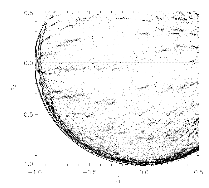
Figure 13: Upper: Contributions of the first 2 eigen-spectra to the 59136 created spectra with given stellar velocity dispersion, stellar populations, signal-to-noise ratios. The three thick lines are the contours of number density ($n$) of all DR1 galaxies with levels of $\lg(n)=1,2,3$. Lower: rms disagreement between the measured and input velocity dispersion of the 12,820 created spectra with given stellar velocity dispersion, stellar population, and signal-to-noise ratio.

The spectra of all galaxies in SDSS DR1 ($\sim 1.4\times 10^{5}$ spectra) are fitted with the 9 galactic eigen-spectra with iterative rejection of emission lines and bad pixels (see §4.2). On a personal computer with a CPU of main frequency 2.8 GHz, this procedure takes $\sim$20 hours. The reduced $\chi^{2}$ , namely $\chi^{2}_{\nu}$ (=$\chi^{2}/dof$, where $dof$ is degree of freedom), for 98.8% spectra are less than 1.5, with the peak of the $\chi^{2}_{\nu}$ distribution around 0.96, and the mean $\chi^{2}_{\nu}\sim$1.04, indicating that the fits are quite good (see Fig. 10). Fig. 13 shows the contour of the number density of DR1 galaxies on the $p_{1}^{\prime}$ vs $p_{2}^{\prime}$ plane, where $p_{1}^{\prime}$ and $p_{2}^{\prime}$ are the fractional contributions of the first 2 galactic eigen-spectra to the modeled spectra. On this diagram, 98.6% galaxies in SDSS DR1 locate in the ring with a radius $\sqrt{{p_{1}^{\prime}}^{2}+{p_{2}^{\prime}}^{2}}$ between 0.9 and 1.

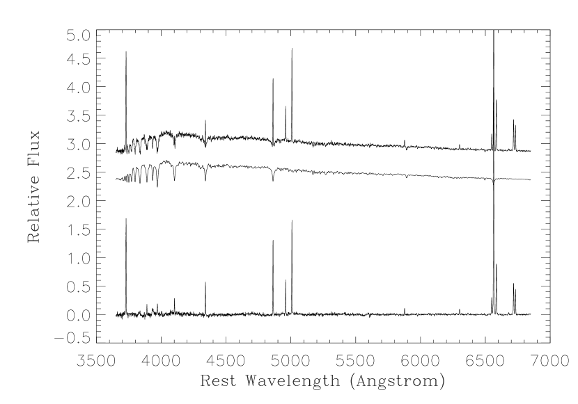
Figure 11: Examples of starlight removal. In each panel, the three lines (from top to bottom) are the observed, the modeled and the starlight-subtracted spectra. For clarity, arbitrary constants are added to the observed and the modeled spectra.

Fig. 11 shows the examples of the fits. Overall residuals in the non-emission line region are consistent with flux fluctuations. The figure also illustrates the importance of the stellar modeling to the emission line measurements. In some of the original spectra, even H$\beta$ is hardly visible, whereas it can be easily measured after the underlying starlight subtracted. Furthermore, the intensities of both H$\beta$ and H$\alpha$ are modified substantially and their ratio changes to be close to the theoretical value.

We would like to point out that, although most of the galactic spectra could be well modeled using this method, the fit is not satisfactory for a small number of spectra ($\lesssim 0.8\%$), out of which, most show peculiar molecular absorption bands and a small portion show obvious Wolf-Rayet feature around 4600-4750 Å. The result is expected because of the lack of very late type stars and Wolf-Rayet stars in the stellar library we used (see Fig. 2). Modeling these objects requires the improvement of the stellar library.

For each spectrum, the best-fitting model is then subtracted from the original spectrum, yielding a pure emission-line spectrum, from which emission line parameters are measured. It is found that the measured equivalent widths of emission lines are well correlated with the coefficients of the eigen-spectra obtained during the modeling, though the latter reflects only the information of the stellar component of galaxies. From SDSS DR1, we select $\sim$500 spectra that have relatively strong emission lines, and use the measured equivalent widths of H$\alpha$ and the modeling coefficients to solve a set of linear equations of

$$EW_{H_{\alpha}}^{j}=\sum_{i=1}^{9}a_{i}c_{ij},$$ (10)

where $EW_{H_{\alpha}}^{j}$ is the measured equivalent width of H$\alpha$ of the $jth$ spectrum, and $c_{ij}$ is the expansion coefficient of the $ith$ eigen-spectrum for the $jth$ spectrum. Using the resultant constants {$a_{i}$}($i=1,9$), the H$\alpha$ equivalent width of each galaxy can be synthesized as a linear combination of the modeling coefficients of the galactic eigen-spectra. Fig. 12 presents the relation between the measured and the synthesized equivalent widths of H$\alpha$ . It can be seen that, for moderately strong emission line, i.e., $EW(H_{\alpha})\lesssim 80$Å, the synthesized value is well correlated with the measured one, while for stronger lines the synthesized values are smaller than the measured.

5.2 Stellar Velocity Dispersion

5.2.1 Tests of the measurement routine

One of the merits of the method presented in this paper is that the stellar velocity dispersion of galaxies can be determined as a byproduct. In order to estimate the accuracy of the measurement of stellar velocity dispersion, we created a set of testing spectra as follows. First, all the 204 stars in STELIB are classified into seven groups according to their spectral types, i.e. O, B, A, F, G, K, and M-type. The average spectra of these groups are then combined by specifying various fractions, to create a set of 462 spectra. The spectra are then broadened by convolution with Gaussian of $\sigma$ in the range of 40-300 km s^-1 . Finally, Gaussian noise is added to the broadened spectra to give S/N = 10-120 per pixel.

The resultant 59,136 spectra with known velocity dispersion, stellar population and S/N ratio are modeled using the method described above. Fig. 13 shows the relative contributions of the first 2 galactic eigen-spectra to the modeled spectra. Clearly only a portion of the created spectra (12,820) locate in the region overlapped with that of SDSS galaxies, and are selected for later test.

The velocity dispersion for the artificial galaxies is measured in the same way as for the really spectra, except that the masked regions for emission lines are selected randomly from the real SDSS spectra. We find that our method can accurately recover the velocity dispersion over the entire range of 40-300 km s^-1 . Figure 13 shows the root-mean-square (rms) disagreement between the measured and input velocity dispersion. As a whole, the measured dispersion is within 35 km s^-1 of the input velocity dispersion for S/N$>$10. For synthesized spectra with $S/N\simeq 20$, the typical value of the SDSS galaxies, the uncertainties of the velocity dispersion measurements is between $\sim$4% and $\sim$10% for higher velocity dispersion ($\sigma_{*}>75$km s^-1 ), while estimates of low velocity dispersions are less accurate ($\sim$20%). For higher signal-to-noise ratios, the measurement errors decrease rapidly. We would like to point out that the accuracy of the stellar velocity dispersion determined using the method presented in this paper is comparable to previous works at high S/N ratio. For the spectra with input dispersion range of 50-300 km s^-1 and S/N=120, Barth, Ho & Sargent (2002) yielded an accuracy within 6 km s^-1 , while this value is less than 5 km s^-1 using our method (see Fig. 13). However, our approach should over-perform these methods using only a couple of absorption lines at low S/N ratio.

5.2.2 Comparison with the SDSS pipeline

Stellar velocity dispersion is also measured by the SDSS spectroscopic pipeline using two different methods: ”Fourier-fitting” and ”Direct-fitting” . The latter is similar to the method presented in this paper except that the SDSS pipeline uses only 32 K and G giant stars in M67 as templates. The SDSS velocity dispersion estimates are obtained by fitting the rest frame wavelength range 4000-7000 Å, and then averaging the estimates provided by the ”Fourier-fitting” and ”Direct-fitting” methods. The error on the final value of the velocity dispersion is determined by adding in quadrature the errors on the two estimates. The typical error is between $\Delta(\lg\sigma_{*})\sim$ 0.02 dex and 0.06 dex, depending on the signal-to-noise of the spectra.

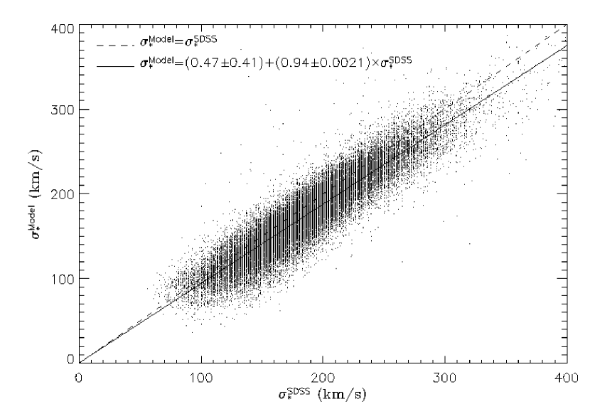
Figure 14: Left: Comparison with stellar velocity dispersion provided by the SDSS pipeline. The SDSS velocity dispersion $\sigma_{*}^{SDSS}$ and that obtained using the present method $\sigma_{*}^{Model}$ for 46229 spectra in SDSS DR1 are plotted (dots). The solid line is the fitted relation and the dashed is that of $\sigma_{*}^{Model}=\sigma_{*}^{SDSS}$. Right: Distribution of stellar velocity dispersion of DR1 galaxies measured by our method: dot: $\sim 4.6\times 10^{4}$ galaxies that have SDSS velocity dispersions (the corresponding SDSS velocity dispersions are plotted in dot-line); dashed: the other $\sim 8.8\times 10^{4}$ galaxies without SDSS velocity dispersion; solid: All the DR1 galaxies.

However, stellar velocity dispersions $\sigma_{*}$ are only measured for spheroidal systems by the SDSS spectroscopic pipeline. The main selection criteria is the PCA classification ”eClass” less than -0.02, typical of spectra of early-type galaxies. Adopting these criteria, $\sim 4.6\times 10^{4}$ spectra of galaxies in SDSS DR1 were chosen to measure $\sigma_{*}$ by the SDSS pipeline. The values determined by the SDSS pipeline are compared with our measurements in Fig. 14 (left panel). The two estimates are almost consistent with each other except that our measurements are systemically a bit smaller than those determined by the SDSS pipeline. This is understandable because our model is expected to fit the spectrum better, reducing the template mismatch problem. The iterative rejection of emission lines in our procedure can also improve the accuracy of the velocity measurement.

In Fig. 14 (right panel), the distribution of the velocity dispersion of this paper and that provided by the SDSS pipeline are presented. In addition to the $\sim 4.6\times 10^{4}$ galaxies, we also measure the rest $\sim 8.8\times 10^{4}$ galaxies whose $\sigma_{*}$ are not provided by the SDSS pipeline. It can be seen that the velocity dispersions of these objects are systematically smaller than that of the $\sim 4.6\times 10^{4}$ early type-galaxies. This is consistent with the general impression that the stellar velocity dispersion of spheroidal systems is generally larger than that of late-type ones. Using the method presented in this paper, the data set of $\sigma_{*}$ is enlarged $\sim 3$ times compared with that provided by the SDSS pipeline. As it is illustrated in Fig 6, by carefully masking the emission-line wavelength range, $\sigma_{*}$ can be reliably determined using our method for most of emission line galaxies.

5.3 Spectral Classification

Galaxy classification plays important role in the study of galaxy formation and evolution. Three methods are often used for this purpose: morphological segregation, rest-frame colors, and direct spectrum-based classifications, while each method has its own unique drawbacks and advantages (Madgwick et al. 2003).

As shown in Fig. 4, the position angle $\theta$ of the stars on the diagram of their relative contributions to the first two eigen-stars are well correlated with the spectral type, suggesting that $\theta$ is a good indicator of stellar types and thus useful for stellar classification. Similarly, most of the galaxies on the diagram of their relative contributions to the first two eigen-galaxies also distribute on the unit circle (see Fig. 8). The corresponding position angle of galaxies is therefore expected to be a good single-parameter classifier of galaxies. However, such a PCA-based classification of galactic spectra is only applicable to small samples, such as the galaxy sample presented in §4.1, because of the required computation expense of implementing PCA on large or very high-dimensional data sets. Nevertheless, we note that there is another similar parameter, namely the position angle $\theta^{\prime}$ of galaxies on the diagram of the contributions of the first two eigen-galaxies to the modeled spectra (the $p_{1}^{\prime}~{}vs~{}p_{2}^{\prime}$ plane; see Fig. 13), which is also a good classifier.

In fact, SDSS DR1 pipeline also provide a spectral classification of galaxies, by cross-correlating with eigen-templates constructed from early SDSS spectroscopic data using PCA method. 5 eigen-coefficients and a classification number are stored in parameters ”eCoeff1-5” and ”eClass”, respectively (Stoughton, et al. 2002). The parameter ”eClass”, based on the expansion coefficients ”eCoeff1”-”eCoeff5”, ranges from about -0.35 to 0.5 for early- to late-type galaxies. Since the sign of the second eigen-spectrum has been reversed with respect to that of the Early Data Release (EDR, see Stoughton et al. 2002), the expression $atan(-eCoeff2/eCoeff1)$ is recommended rather than ”eClass” as the single-parameter classifier . To compare our classifier $\theta^{\prime}$ with that provided by the SDSS pipeline, we randomly select 1000 galaxies from SDSS DR1 and fit their spectra to obtain the modeling coefficients of templates and subsequently the position angles $\theta^{\prime}$. As may be seen clearly in Fig. 15 (left panel), the position angle $\theta^{\prime}$ is actually a good single-parameter classifier, which is well correlated with the classifier $atan(-eCoeff2/eCoeff1)$ provided by the SDSS pipeline. This is understandable because both of the classifiers are obtained based on PCA. Moreover, our classifier $\theta^{\prime}$ is also well correlated with the mean velocity dispersion $<\sigma_{*}>$ of the 1000 galaxies (see the right panel in Fig. 15), with smaller $\theta^{\prime}$ corresponding to larger velocity dispersion, thus to earlier type galaxies.

Using the rest-frame colors, Strateva et al. (2001) studied the color distribution of a large uniform sample of galaxies detected in SDSS commissioning data and showed that the $g^{*}-r^{*}$ versus $u^{*}-g^{*}$ color-color diagram is strongly bimodal, with an optimal color separation of $u^{*}-r^{*}=2.22$ and the two peaks corresponding roughly to early- (E, S0, and Sa) and late-type (Sb, Sc, and Irr) galaxies. As can be seen clearly in Fig. 16, the early- and late-type galaxies separated by $u^{*}-r^{*}=2.22$ could be also well classified using our single-parameter classifier $\theta^{\prime}$, indicating that $\theta^{\prime}$ might be also compatible for galactic classification.

5.4 Near-infrared SED

Once a spectrum has been modeled using the 9 galactic eigen-spectra, the contributions of the 24 eigen-stars to the modeled spectrum can be conveniently obtained. Since the 24 stellar eigen-spectra contain the infrared information of the 204 original stars (§3), the infared fluxes at J,H and K_s bands could be re-constructed from a set of expansion coefficients

We test reliability of the stellar SED in the near infrared using this method on a set of ”average” spectra of normal galaxies along the Hubble diagram between E and Sc between 0.1 and 2.4 $\mu$m, presented by Mannucci et al. (2001) . The composited spectra were derived from 28 nearby galaxies, and overall precision of the calibrated spectra is about 2 per cent.

The five spectra are modeled using the 9 templates and the results are presented in Figure 17. As can be seen, the modeled infrared fluxes are systematically lower than the observed one by $\sim 10\%$ for E to Sb types, and 30% for Sc galaxies. The discrepancy is understandable as the observed infrared flux includes additional emission from hot dust, presumably caused by stochastic heating of small grains by UV photons, which is expected to increase both with the dust content and young stellar population along the Hubble sequence. Besides, if dust extinction is patched, the single E(B-V) correction will under-estimate the true extinction in the optical. Nevertheless, we argue that the result of our method could give reliable information of starlight at infrared band for a galaxy (especially for early types), by only using its optical spectrum.

5.5 Average Reddening

Our solution also yields an average stellar reddening $E(B-V)^{*}$ for each galaxy (see §4.2). The extinction is quite significant for 85.5% galaxies, with the $E(B-V)^{*}$ in the range of 0.01-0.5. On the other hand, the internal reddening can be also estimated using Balmer decrements of the emission lines from Hii region. To check the consistency of the two estimates, we select a sample of $\sim 10^{4}$ Hii galaxies from SDSS DR1 adopting the criteria of Kewley et al. (2001):

$$\log{\big{(}\frac{[\mbox{O {\sc iii}}]\lambda 5007}{\mbox{H}\beta}\big{)}}<\frac{0.61}{\log([\mbox{N {\sc ii}}]/\mbox{H}\alpha)}+1.19.$$ (11)

Using the effective extinction curve $\tau_{\lambda}=\tau_{V}(\lambda/5500$Å$)^{-0.7}$, which was introduced by Charlot & Fall (2000), the color excess arising from attenuation by dust in the selected galaxy $E(B-V)^{Balmer}$, can be written:

$$E(B-V)^{Balmer}=A_{V}/R_{V}=1.086\tau_{V}/R_{V},$$ (12)

$$\tau_{V}=-\frac{\ln[F(\mbox{H}\alpha)/F(\mbox{H}\beta)]-\ln[I(\mbox{H}\alpha)/I(\mbox{H}\beta)]}{(\lambda_{\mbox{H}\alpha}/5500)^{-0.7}-(\lambda_{\mbox{H}\beta}/5500)^{-0.7}},$$ (13)

where $I(\mbox{H}\alpha)/I(\mbox{H}\beta)$=2.87 is the intrinsic Blamer flux ratio , $F(\mbox{H}\alpha)/F(\mbox{H}\beta)$ the observed Balmer flux ratio , $\tau_{V}$ the effective V-band optical depth, $\lambda_{\mbox{H}\alpha}$=6563Å, $\lambda_{\mbox{H}\beta}$=4861Å, and $R_{V}$=3.1. For objects with the observed flux ratio $F(\mbox{H}\alpha)/F(\mbox{H}\beta)<$ 2.87, $\tau_{V}$ is set to zero. The resultant $E(B-V)^{Balmer}$ vs $E(B-V)^{*}$ is plotted in Fig. 18. Although the dispersion of $E(B-V)^{*}$ is large ($\sim$ 0^m.2), the tendency is apparent: the $E(B-V)^{*}$ increases with increasing $E(B-V)^{Balmer}$, and the former is systemically smaller than the latter, which is also consistent with previous works (e.g Calzetti, Kinney, & Storchi-Bergmann 1994).

6 Summary

We have developed an empirical method for modeling the stellar spectrum of galaxies. The absorption-line templates with zero velocity dispersion are constructed based on two successive applications of Principal Component Analysis (PCA), first to 204 stars in the stellar library STELIB, then to a uniform sample of galaxies selected from SDSS DR1. With 9 templates, we can fit quite well the stellar spectra of galaxies in the SDSS DR1. As byproducts, the stellar velocity dispersion, the near-infrared SED, the spectral type, and the average reddening are determined simultaneously. For a spectrum of S/N=20, typical for SDSS galaxies, the velocity dispersion can be determined to accuracy of $\sim$4-10% at larger value ($>$75 km s^-1), and $\sim$20% at low dispersion ($<$75  km s^-1). The average reddening of stellar light is correlated, and is systematically smaller than that derived from Balmer decrements of Hii region. After stellar light have been subtracted, emission line parameters are measured for all galaxies. An interesting result is that the measured equivalent width of H$\alpha$ is well correlated with the modeling coefficients of the templates, suggesting that these coefficients also contain information of current star formation rate.

The success of this approach could be understood from the following aspects. First, two applications of PCA highly concentrate the most prominent features from both the stellar library and the galaxy sample into the first few galactic eigen-spectra, and hence significantly reduce the number of the final templates. This makes the procedure of spectral modeling much quicker, and the results much more stable and reliable, in particular, when dealing with large datasets, in comparison with using direct stellar populations. Second, the templates derived from the large galaxy sample with full coverage of spectral type, ensure a close match to the true underlying stellar population of different type galaxies, including emission line galaxies that contain much young stellar component. As a result, the modeled spectra reflect the true information on the stellar population in galaxies, and provide useful clues for their spectral classifications. Third, the templates are not obtained directly from the observed galactic spectra, but from the modeled one with zero velocity dispersion, and therefore could match better the absorption line profile of galaxies. Finally, the extended wavelength coverage (from optical to near-infrared) in the templates enables us to study the stellar component at NIR band, using only the optical spectrum of galaxies.

It should be pointed out that there are still rooms for improvement of this method. First, lack of very late type stars limits our application of templates in modeling a small fraction of galaxies which show prominent, peculiar molecular absorption features. This can be improved by adding very late type stars to the stellar library. Second, implication of each PCs should be tackled, by setting a relation between fitting coefficients of templates and stellar population. This may be addressed by combining the stellar population synthesis with the PCA method, which is still under investigation.

Figure 2: Distribution of the spectral types of the STELIB library (cross) and that of the 204 stars used in this paper (squared). Note that, out of the total 255 stars in STELIB, Feige110 (dwarf A), LTT4364 (dwarf Carbon), and 6 WC- or WN-type stars are not plotted in this figure.

Figure 3: The first three eigen-spectra of the stellar library. The solid lines represent the spectra in visible range, while the cross points are the J, H, and K_s fluxes. Arbitrary constants are added to the scaled spectra for clarity.

Figure 4: Left: Relative contributions of the 204 stars to the first two eigen-stars. Right: The position angles $\theta$ of the 204 stars in the $p_{1}$ vs $p_{2}$ plane (left panel), as a function of their spectral types. $\theta$ is measured anticlockwise from the dashed horizontal line in the left panel.

Figure 5: An example of selecting galaxy sample on color-color diagrams. $m_{6}$, $m_{12}$, and $m_{18}$ are the magnitudes derived from the modeled spectrum of galaxies (see the text for details). dot: 7098 galaxies of low redshift and high spectral S/N ratio in SDSS DR1. cross: the galaxies selected on this diagram.

Figure 6: An example of masked regions of emission lines during the spectral modeling. The thine line is the observed spectrum of SDSS J1308+0020, and the thick is the best-fitting spectrum. The dashed lines denote the masked regions.

Figure 7: The spectra of the first three eigen-galaxies. The solid lines represent the spectra in visible range, while the cross points are the J, H, and K_s fluxes. Arbitrary constants are added to the scaled spectra for clarity.

Figure 8: Relative contributions of the 1016 galaxy templates to the first two eigen-galaxies.

Figure 9: F-test to choose the number of significant eigen-spectra of galaxies.

Figure 10: Distribution of reduced $\chi^{2}$ for spectral modeling of all galaxies in SDSS DR1. The vertical line marks the mean value of $\chi^{2}/dof$=1.04.

Figure 12: A comparison of the H$\alpha$ EW as derived by a Gaussian fit to the H$\alpha$ line in the starlight-subtracted spectrum and by synthesizing the modeling coefficients of templates.

Figure 15: Left: The position angles $\theta^{\prime}$ of the 1000 galaxies on the $p_{1}^{\prime}$ vs $p_{2}^{\prime}$ diagram (left panel in Fig. 13; $\theta^{\prime}$ is measured anticlockwise from the positive Y-axis) versus their atan(eCoeff2/eCoeff1) provided by the SDSS pipeline. Right: Mean velocity dispersion of 1000 galaxies as a function of their position angles on the $p_{1}^{\prime}$ vs $p_{2}^{\prime}$ diagram.

Figure 16: Left: Color-Color diagram for 1000 galaxies. cross: galaxies with position angle $\theta^{\prime}>120^{\circ}$; square: galaxies with $\theta^{\prime}<120^{\circ}$ (see Fig. 13). The solid line denotes $u^{*}-r^{*}=2.22$ . Right: $u^{*}-r^{*}$ vs $\theta^{\prime}$ (see Fig. 13) for the 1000 galaxies. The horizontal line denotes $u^{*}-r^{*}=2.22$.

Figure 17: Modeling the ”average” spectra of normal galaxies along the Hubble diagram between E and Sc. dashed lines: the ”average” spectra. solid lines: the modeled optical spectra. cross: the modeled J, H and K fluxes. Arbitrary constants were added to the scaled spectra for clarity.

Figure 18: Mean color excess $E(B-V)^{Balmer}$ estimated from the flux ratio of Balmer lines $f(H_{\alpha})/f(H_{\beta})$ vs the modeled $E(B-V)^{Model}$ obtained using the method presented in this paper, for $\sim 10^{4}$ Hii regions or starburst galaxies in SDSS DR1. The bin size of the color excess is so chosen as to have at least 30 galaxies in each bin. The horizontal line in the upper-left corner is the typical error of $E(B-V)^{Model}$.

References

- Abazajian et al. (2003) Abazajian, K., et al. 2003, AJ, 126, 2081
- Barth, Ho, & Sargent (2002) Barth, A. J., Ho, L. C., & Sargent, W. L. W. 2002, AJ, 124, 2607
- Bruzual & Charlot (2003) Bruzual, G. & Charlot, S. 2003, MNRAS, 344, 1000
- Calzetti et al. (2000) Calzetti, D. et al. 2000, ApJ, 533, 682
- Calzetti, Kinney, & Storchi-Bergmann (1994) Calzetti, D., Kinney, A. L., & Storchi-Bergmann, T. 1994, ApJ, 429, 582
- Charlot & Fall (2000) Charlot, S., & Fall, S. M. 2000, ApJ, 539, 718
- Charlot, Worthey, & Bressan (1996) Charlot, S., Worthey, G., & Bressan, A. 1996, ApJ, 457, 625
- Combes et al. (2002) Combes, F. et al. 2002, Galaxies and Cosmology-2nd edn, Heidelberg:Springer-Verlag
- Connolly et al. (1995) Connolly, A. J., Szalay, A. S., Bershady, M. A., Kinney, A. L., & Calzetti, D. 1995, AJ, 110, 1071
- Danks & Dennefeld (1994) Danks, A. C., & Dennefeld, M. 1994, PASP, 106, 382
- Dong et al. (2004) Dong, X. B., et al. submitted to ApJ.
- Faber (1972) Faber, S. M. 1972, A&A, 20, 361
- Gunn & Stryker (1983) Gunn, J. E., & Stryker, L. L. 1983, ApJS, 52, 121
- Hao, Strauss, & SDSS Collaboration (2002) Hao, L., Strauss, M., & SDSS Collaboration 2002, American Astronomical Society Meeting, 201,
- Heck et al. (1984) Heck, A. et al. 1984, A&AS, 57, 213
- Ho, Filippenko, & Sargent (1997) Ho, L. C., Filippenko, A. V., & Sargent, W. L. W. 1997, ApJS, 112, 315
- Jacoby, Hunter & Christian (1984) Jacoby, G. H., Hunter, D. A., & Christian, C. A. 1984, ApJS, 56, 257
- Kennicutt (1992) Kennicutt, R. C. 1992, ApJS, 79, 255
- Kewley et al. (2001) Kewley L. J. 2001, ApJ, 556, 121
- Kiehling (1987) Kiehling, R. 1987, A&A, 69, 465
- Kong, Charlot, Weiss, & Cheng (2003) Kong, X., Charlot, S., Weiss, A., & Cheng, F. Z. 2003, A&A, 403, 877
- Kurucz (1992) Kurucz, R. L. 1992, in IAU Symp., 149, 255
- Le Borgne et al. (2003) Le Borgne, J.-F. et al. 2003, A&A, 402, 433
- Lejeune, Cuisinier, & Buser (1997) Lejeune, T., Cuisinier, F., & Buser, R. 1997, A&AS, 125, 229
- Lejeune, Cuisinier, & Buser (1998) Lejeune, T., Cuisinier, F., & Buser, R. 1998, A&AS, 130, 65
- Madgwick et al. (2003) Madgwick, D. S., et al. 2003, ApJ, 599, 997
- Mannucci et al. (2001) Mannucci, F., Basile, F., Poggianti, B. M., Cimatti, A., Daddi, E., Pozzetti, L., & Vanzi, L. 2001, MNRAS, 326, 745
- Pickles (1985) Pickles, A. J. 1985, ApJ, 296, 340
- Pickles (1998) Pickles, A. J. 1998, PASP, 110, 863
- Robert et al. (1993) Robert, C., Leitherer, C., & Heckman, T. M. 1993, ApJ, 418, 749
- Serote, Boisson & Joly (1996) Serote, R. M., Boisson, C., & Joly, M. 1996, A&AS, 117, 93
- Skrutskie et al. (1997) Skrutskie, M. F. et al. 1997, ASSL Vol. 210: The Impact of Large Scale Near-IR Sky Surveys, 25
- Sodr & Cuevas (1997) Sodr, L. & Cuevas H. 1997, MNRAS, 287, 137
- Stoughton et al. (2002) Stoughton, C., et al. 2002, AJ, 123, 485
- Strateva et al. (2001) Strateva, I., et al. 2001, AJ, 122, 1861
- Tinsley (1967) Tinsley, B. M. H. 1967, Ph.D. Thesis
- Walborn et al. (1995) Walborn, N. R. et al. 1995, IUE Atlas of B-type Spectra From 1200 to 1900 Å, 1155
- Westera et al. (2002) Westera, P., Lejeune, T., Buser, R., Cuisinier, F., & Bruzual, G. 2002, A&A, 381, 524
- York et al. (2000) York, D. G. et al. 2000, AJ, 120, 1579