The Magellanic Clouds Photometric Survey: The Large Magellanic Cloud Stellar Catalog and Extinction Map

Abstract

We present our catalog of $U$, $B$, $V$, and $I$ stellar photometry of the central $64$ deg² area of the Large Magellanic Cloud. Internal and external astrometric and photometric tests using existing optical photometry ($U$, $B$, and $V$ from Massey’s bright star catalog and $I$ from the near-infrared sky survey DENIS) are used to confirm our observational uncertainty estimates. We fit stellar atmosphere models to the optical data to check the consistency of the photometry for individual stars across the passbands and to estimate the line-of-sight extinction. Finally, we use the estimated line-of-sight extinctions to produce an extinction map across the Large Magellanic Cloud, confirm the variation of extinction as a function of stellar population, and produce a simple geometrical model for the extinction as a function of stellar population.

1. Introduction

A galaxy’s star formation history is encoded within its stellar populations. Outside of our own galaxy, the Magellanic Clouds provide our most detailed view of galaxies that are still vigorously forming stars. We present the catalog of stellar photometric data from the Magellanic Clouds Photometric Survey (MCPS) for the entire Large Magellanic Cloud (LMC) survey region (roughly $8.5^{\circ}\times 7.5^{\circ}$, with the longer direction corresponding to the east-west axis). Our data are either deeper, cover a wider area, or include a larger number of filters (the inclusion of $U$ is particularly important for studies of dust and young stellar populations) than available optical catalogs.

In addition to describing and providing the catalog, we construct and analyze extinction maps of the LMC. As we demonstrated for a portion of the LMC (Zaritsky, 1999) and for the SMC (Zaritsky et al., 2002), the extinction properties in the Clouds vary both spatially and as a function of stellar population. Therefore, for many scientific purposes the catalog alone is insufficient, one must correct the observed magnitudes and colors for a complex extinction pattern. We describe the MCPS in §2, use the photometry to generate extinction maps of the LMC for two different stellar populations in §3, model the relative distributions of young stars, old stars, and dust in §4, and summarize in §5.

2. The Data

The data come from Magellanic Cloud Photometric Survey, originally described by Zaritsky et al. (1997). Using the Las Campanas Swope telescope (1m) and the Great Circle Camera (Zaritsky et al., 1996) with a 2K CCD, we obtained drift-scan images for both Magellanic Clouds in Johnson $U,B,V,$ and Gunn $i$. The effective exposure time is between 3.8 and 5.2 min for LMC scans and the pixel scale is 0.7 arcsec pixel^-1. Typical seeing is $\sim$1.5 arcsec and scans with seeing worse than $\sim$ 2.5 arcsec are not accepted. Magnitudes are placed on the Johnson-Kron-Cousins photometric system (Landolt, 1983, 1992). Scan images from observing runs from October 1995 to December 1999 are included in this catalog. Additional pointed observations were performed in December 2001 to fill in for unacceptable data from earlier observations. The data are reduced using a pipeline that utilizes DAOPHOT II (Stetson, 1987) and IRAF. Only stars with both $B$ and $V$ detections are included in the final catalog.

Details of the reduction procedure, construction of the catalog, and quality assurance are presented by Zaritsky et al. (2002). Because the SMC and LMC data were taken concurrently, the quality of the two datasets is identical. We present only a cursory description of the procedure here. The pipeline for reducing individual scans is a fairly standard application of DAOPHOT. Each of the 76 scans ($\times$ 4 for the four filters), which are 11000 pixels long and 2011 pixels wide, is divided into 11 by 2 subscans that are roughly 1100 by 1100 pixels, with overlap between the subscans that enables us to compare the results from the independent photometric reductions. The result of the reduction pipeline is a catalog of instrumental photometry for each detected star in each filter and its right ascension and declination. We derive the astrometric solution from a comparison to stars in the Magellanic Catalogue of Stars (MACS; Tucholke et al. (1996)), whose coordinates are on the FK5 system.

We match the instrumental magnitudes of stars in different filters using a positional match that associates the nearest star on the sky within an aperture that is 3 times either the positional rms of the astrometric standards in that subscan or 1.2 arcsec, whichever is larger. The $V$ frame is used as the reference and only stars that have a match in the $B$ frame are retained for the final catalog. In crowded areas it is possible that the “nearest” star in one filter is not the correct match to the $V$ reference because of the uncertainties in the astrometric solution. We see some evidence of this problem when comparing to other data and when fitting atmospheric models (we find stars with highly anomalous colors). Except near the faint limit of the catalog or in extremely crowded regions, this issue appears to be a minor problem. These errors can be estimated reliably using artificial star simulations.

One significant difference bewteen the photometric solution of the LMC and SMC data, is that for the LMC data we do not automate the adjustment of the scan-to-scan photometry. We find that the photometry among scans is generally consistent, and only a few manual adjustment of scan zeropoints were necessary. These were implemented to remove obvious discrepancies observed in a map of the density of red clump stars (for an example see Figure 1). The adjustment of specific individual scans avoids the potential for systematic drift present in an automated procedure.

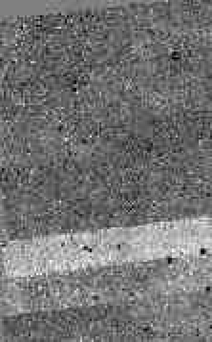
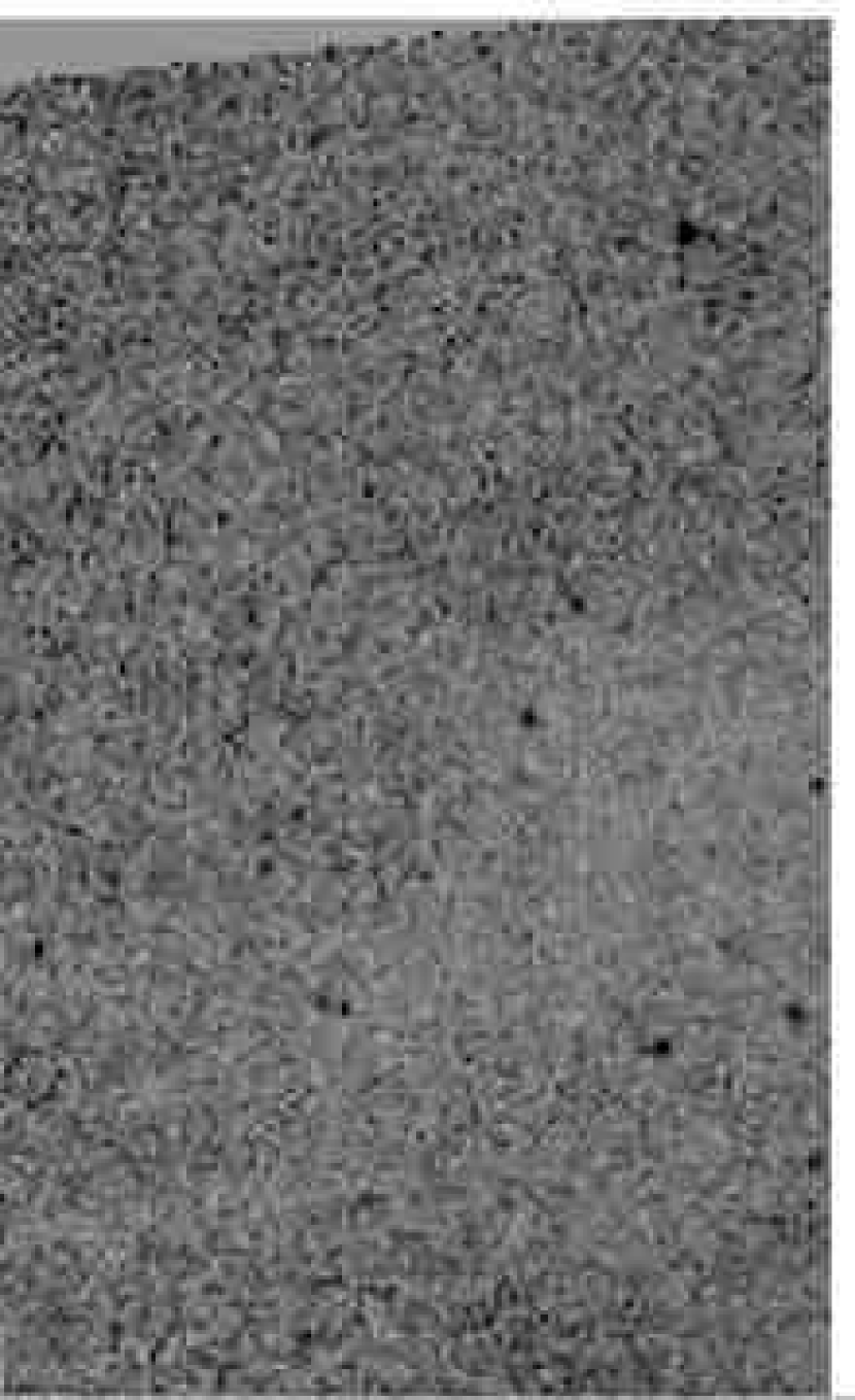
Figure 1.— A section of the red clump stellar density map for the LMC. The left panel contains the I-band photometry with no corrections, the right panel contains the photometry after correction.

We present the catalog of astrometry and photometry for 24,107,004 stars as an ASCII table (see Table 1 for a sample). Columns 1 and 2 contain the right ascension and declination (J2000.0) for each star. Columns 3-10 contain the pairings of magnitudes and uncertainties for $U$, $B$, $V$, and $I$ magnitudes. The last column is a quality flag that is described in Table 2, based on comparisons to Massey’s (2001) catalog and our fitting of the spectral energy distribution (§3). A $V$ band stellar density map of the LMC constructed from the catalog using stars with $16<V<20$ is shown in Figure 3. The digital catalogs allow one to make analogous images for a variety of populations (for an example of the distribution of young and old stars in the LMC, as done for the SMC by Zaritsky et al. (2000), see Figure 2).

Table 1The MCPS Catalog for the Large Magellanic Cloud

RA	Dec	$U$	$\sigma_{U}$	$B$	$\sigma_{B}$	$V$	$\sigma_{V}$	$I$	$\sigma_{I}$	Flag
4.490203	$-$72.22987	.000	.000	20.740	.060	19.746	.054	18.535	.063	0
4.490215	$-$72.19868	.000	.000	22.694	.271	22.788	.310	.000	.000	0
4.490216	$-$72.28524	.000	.000	21.646	.099	20.894	.071	.000	.000	0
4.490218	$-$72.37505	.000	.000	21.455	.107	21.050	.086	20.795	.167	0
4.490222	$-$72.29113	.000	.000	21.379	.076	21.298	.106	.000	.000	0
4.490228	$-$72.09232	.000	.000	21.668	.104	20.700	.067	20.114	.087	0
4.490231	$-$72.09853	21.724	.410	21.221	.078	20.740	.062	20.015	.099	0
4.490231	$-$72.17493	.000	.000	22.277	.202	22.220	.213	21.657	.271	0
4.490236	$-$72.18102	20.326	.168	20.013	.070	19.134	.078	18.055	.073	10
4.490241	$-$72.09316	21.588	.384	22.491	.231	22.009	.176	.000	.000	0
4.490252	$-$72.13191	.000	.000	23.283	.378	22.997	.356	.000	.000	0
4.490256	$-$72.13083	20.287	.140	20.379	.061	19.989	.055	.000	.000	0
4.490261	$-$72.20712	.000	.000	22.687	.318	23.412	.495	.000	.000	0
4.490273	$-$72.18983	.000	.000	22.368	.201	21.895	.135	21.320	.271	0
4.490280	$-$72.40957	.000	.000	21.811	.120	21.296	.113	.000	.000	0

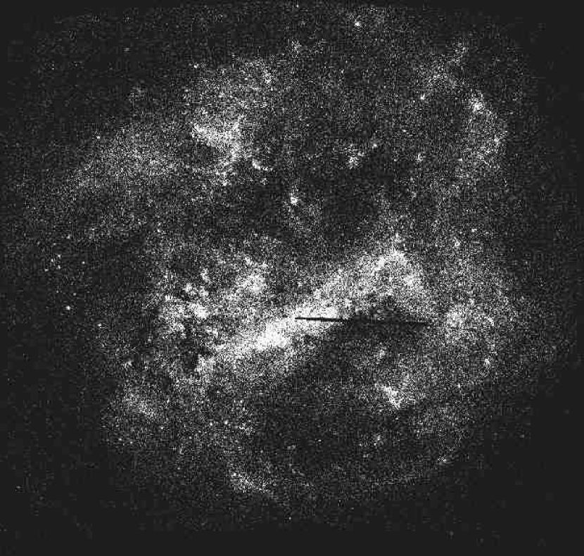
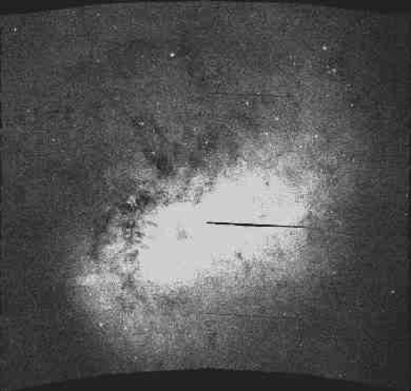
Figure 2.— The stellar density map of the LMC for the young population ($V<18.5$ and $-0.2<B-V<0.3$) in the left panel and an old population ($V<19.1$ and $0.7<B-V<1.5$) in the right panel. North is up and East is to the left. The image shows the entire $\sim 8.5^{\circ}\times 7.5^{\circ}$ survey region.

Table 2MCPS Catalog Flags

Description	Value
Replaced with Massey’s (2001) photometry & astrometry	1
Colors successfully fit with stellar atmosphere model	10
Colors poorly fit with stellar atmosphere model	20

The magnitude limit of the survey varies as a function of stellar crowding. We find little visible evidence for incompleteness at $V<20$ (Figure 3), but the scan edges and different scan sensitivities become visible when plotting the stellar surface density for stars with $20<V<21$ (Figure 4). The $U$ and $I$ data are incomplete at brighter magnitudes than the $B$ and $V$ data. The $U$ and $I$ photometry, even in sparse areas, is severely incomplete below $U=21.5$ and $I=22$ (comparable limits in the two other bands are $B=23.5$ and $V=23$). Any statistical analysis of this catalog fainter than $V<20$ requires artificial star tests to determine incompleteness, which is becoming significant at these magnitudes.

2.1. Photometric and Astrometric Accuracy

We presented extensive tests of the photometry and astrometry of the MCPS in Zaritsky et al. (2002). However, we revisit some of those here for completeness. One particularly useful internal test is based on a map of the red clump mean luminosity. We calculate the mean magnitude of the red clump in 50 $\times$ 50 arcsec boxes over the survey region. Although large-scale variations in the mean magnitude may truly exists (for example due to a tilt of the LMC relative to a constant-distance surface; see van der Marel & Cioni (2001) for a demonstration of an analogous effects with the red giant branch tip magnitude), any localized variation, in particular one that traces scan or subscan boundaries, reveals a problem region. In Figure 5 we show the maps of the deviations from the mean red clump magnitude, for each filter. There are various important features in these panels. First, all four panels show increased noise toward the edges because there are fewer clump stars at large radii from the LMC and contamination for foreground Galactic stars is proportionally greater. Second, the $U$ and $I$ band frames show more structure that follows scan and subscan edges. Although we interactively corrected the most egregious of these (§2), we did not correct subscans within the bar region nor did we apply correction in cases where the correction needed was ambiguous. Recall that the $U$ and $I$ images are not as deep as the $B$ and $V$ images, so that some of the differences could be due to senstivity and completeness variations among scans (the clump stars are near the $U$ magnitude limit). Third, there are large spatial scale variations that trace the bar, and repeat in the various colors. These are real variations in the mean magnitude of clump stars, presumably either due to physical effects (geometry, population differences, or variable extinction). We conclude that with the exception of some regions in the $U$ and $I$ band data, the photometry is self consistent among scans. The worst variations seen in the $U$ band correspond to $\sim$ 0.1 mag.

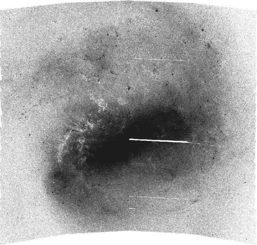
Figure 3.— The stellar density map of the LMC for stars with $16<V<20$. North is up and East is to the left. The image shows the entire $\sim 8.5^{\circ}\times 7.5^{\circ}$ survey region. The nearly-horizontal white lines are caused by slight gaps between scans, which occurred if either the $V$ or $B$ scan was slightly misaligned. The irregular patchiness is due to extinction that is confirmed in §3.

In Zaritsky et al. (2002) we compared our photometry to various existing catalogs. The quality of the photometry presented here is identical since the LMC and SMC data were taken concurrently. However there is one issue that requires further comment. Massey (2002) has produced a photometric catalog ($U,B,V$ and $R$) of bright stars in the LMC. In particular, because of his interest in the upper main sequence, he pays acute attention to obtaining accurate $U$-band photometry for young LMC stars, which is often difficult because of the lack of blue ($U-B<0.0$) standards. He found that the combination of filter, CCD passbands, and the gravity sensitivity of the Balmer jump produced rather complex color transformation between his $U$-band observations and the standard Johnson system. Specifically, he required a second order color-term to correct his magnitudes.

We had previously used his uncorrected photometry to correct our $U$-band photometry (a slightly linear color term was added to place our photometry on his system, which was more extensively calibrated than our $U$-band system; Zaritsky et al. (2002)). However, between that correction and his publication of the catalog, he identified the additional complication in the calibration of the $U$-band data mentioned above. Because the effect appears to arise from the application of a calibration based on dwarf stars to the supergiants at these magnitudes in the LMC, our expectation is that our published photometry is correct for dwarfs, but that the second order color term is required for supergiants. Because most of the stars in the catalog are not blue supergiants, our general results should be unaffected. This conclusion is supported indirectly by the results of our modeling of the SMC population, where we found good agreement with the overall photometry and models (Harris & Zaritsky, 2003). Nevertheless, detailed photometry of the upper main sequence is more uncertain than quoted in our original catalog (Zaritsky et al., 2002).

To examine this issue further, we match our photometry of LMC stars to that of Massey (2002). We match stars brighter than $V=15$ in Massey’s catalog to stars in the MCPS by finding the star in the MCPS within 7.5 arcsec that has the closest $V$ magnitude, as was done for the SMC data. The selection of the search radius is a compromise between assuring that the search finds the corresponding star while moderating the incidence of false matches. Because the bright star catalog has a relatively low density on the sky, we use a large search radius. As expected, we find that our uncorrected $U$ magnitudes have a strong color term relative to those of Massey (see Figure 6). We can correct our magnitudes by roughly fitting a second order $B-V$ color term, which produces the second panel in Figure 6. The correction to our $U$ photometry is $\Delta U=-0.5(B-V-0.7)^{2}+0.23$ if the $(B-V)<1$ and $\Delta U=0.05$ otherwise. The panels on the right hand side of the Figure demonstrate that the correction does indeed decrease the scatter between the two sets of measurements, but the systematic error is still as large as 0.1 mag at certain values of $B-V$. Given the uncertainty of which stars the correction should be applied to due to the gravity sensitivity, we have chosen to not apply the correction to our data as presented in the catalog. However, we will present results in the discussion of derived extinctions with and without the correction. We find that whether the correction is applied or not does not affect our results.

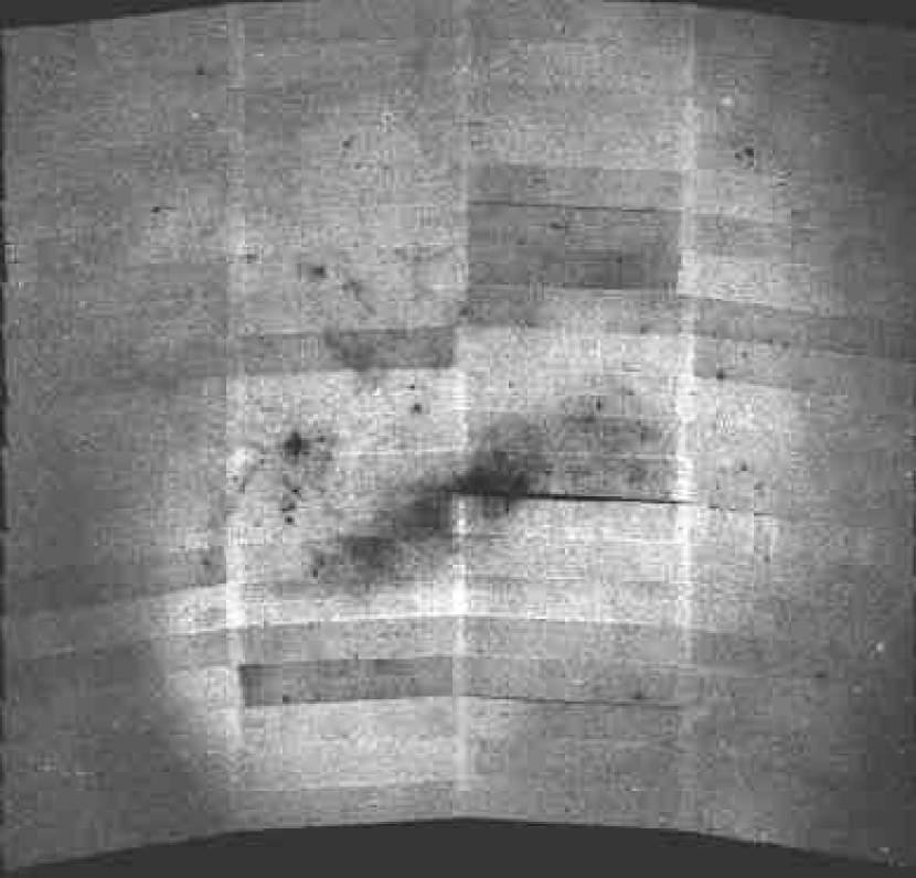
Figure 4.— Stellar density map of stars with $20<V<21$. Various signs of incompleteness and double detections that were unmatched are evident. The scan-to-scan variations reflect varying completeness limits due to seeing variations. Bright regions of overlap between frames show the incidence of false detections. The dark patches along the bar and the region of 30 Doradus show crowding compleness limits.

Stars in our catalog that are brighter than 13.5 in $B$ or $V$ are prone to substantial photometric uncertainty (Zaritsky et al., 2002). In the SMC catalog, we replaced the photometry and astrometry for stars brighter than this limit with those of Massey (2002). However, the Massey catalog for the LMC covers only about a quarter of the area that ours covers. Therefore, most of our stars brighter than 13.5 in $B$ or $V$ have suspect photometry and astrometry. We have, when possible, replaced our photometry with Massey’s, applying the mean photometric offsets found between the MCPS and Massey’s catalog, to Massey’s data. To indicate which stars do have corrected photometry the catalog includes a flag (see Table 2 for description of the quality flags). The photometry and astrometry of 10912 stars are corrected using Massey’s catalog.

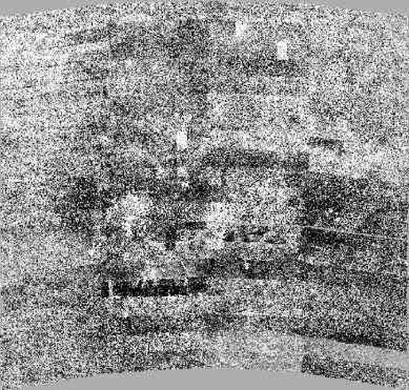
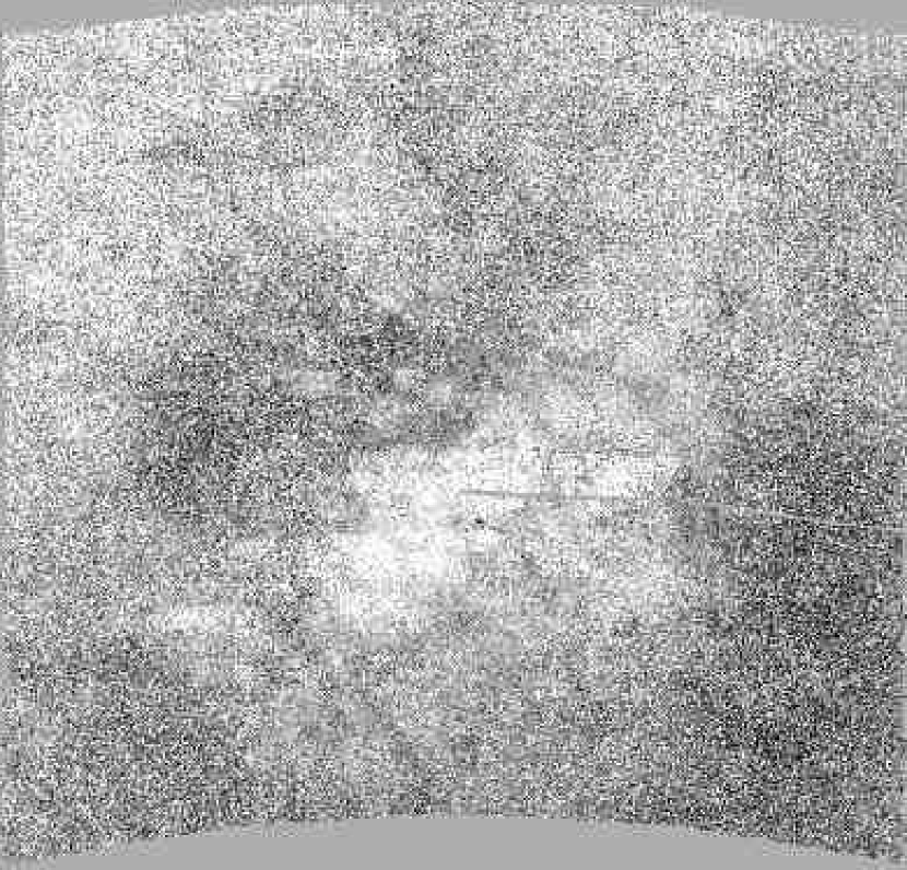
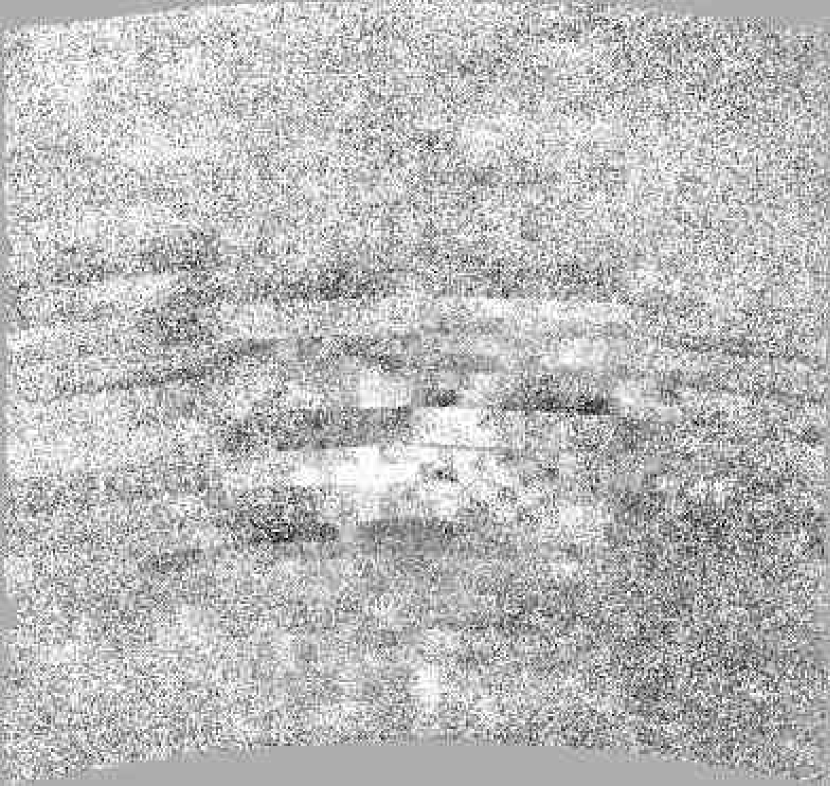
Figure 5.— Comparison of mean red clump magnitudes in U (top left), B (top right), V (bottom left), and I (bottom right). Greyscale ranges from $-$0.3 to 0.3 mag. The entire survey region is shown.

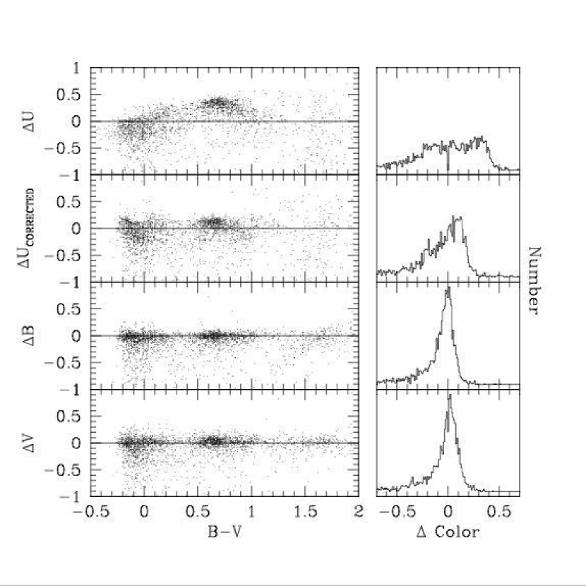
Figure 6.— The comparison of magnitudes as a function of stellar color between the Massey survey and the MCPS. The upper panel shows the results from the original $U$ band photometry, the second panel shows the corrected $U$ band photometry.

Figure 7.— The comparison of DENIS $I$ band catalog with our data. The panel in the left illustrates the astrometric differences for matched stars with $I$-band magnitudes. The panel in the right shows the distribution of differences in $I$ magnitudes between the two surveys.

Finally, we compare our $I$-band photometry to that in the DENIS catalog. Although the DENIS catalog is primarily an IR catalog, it contains an $I$ band channel and Cioni et al. (2000) present a point-source catalog in the regions of the Magellanic Clouds. We use a search aperture of 3.5 arcsec for matches (smaller than that for comparison to the bright star catalog because of the increased stellar density). The distribution of astrometric and photometric differences for matched stars are plotted in Figure 7. In agreement with our previous results, we find that the astrometric accuracy is subpixel for the majority of the matches. The mean difference is 0.45 arcsec. For matched stars whose magnitude agree to within 1 magnitude, the mean photometric difference between the two surveys is $0.01$ mag.

3. Extinction Properties

A comparison between stellar atmosphere models and observed colors can be used to infer the extinction toward individual stars (Grebel & Roberts, 1995; Zaritsky, 1999). We use the models of Lejeune et al (1997) and our $U,B,V$, and $I$ photometry to measure the effective temperature, $T_{E}$, of the star and the line-of-sight extinction, A_V, in the manner described by Zaritsky (1999). We adopt a standard Galactic extinction curve (Schild, 1977), which is acceptable for the LMC over the optical wavelength region (see Gordon et al. (2003)). The model fitting is least degenerate between $T_{E}$ and A_V for stars with derived temperatures in the ranges $5500{\ \rm K}\leq T_{E}\leq 6500{\ \ \rm K}$ and $12,000{\ \rm K}\leq T_{E}\leq 45000{\ \rm K}$. Therefore, we construct A_V maps of the LMC from the line-of-sight A_V measurements to the set of “cool” stars ($5500{\ \rm K}\leq T_{E}\leq 6500{\ \rm K}$) and the set of “hot” stars ($12000{\ \rm K}\leq T_{E}\leq 45000{\ \rm K}$) with good quality photometry in all four filters ($\sigma_{U}<0.4$, $\sigma_{B}<0.2$, $\sigma_{V}<0.2$, $\sigma_{I}<0.2$) and good model fits ($\chi_{\nu}^{2}<3$). In addition to these criteria, we imposed a reddening-independent magnitude cut ($V<19.0+3.2\times(B-V)$). We caution however, that although the magnitude cut is reddening-independent, there is a bias in the catalog against highly extincted stars simply because the catalog itself is magnitude limited. Stars which satisfy the photometric criteria and have an acceptable model fit ($\chi_{\nu}^{2}<3$) have a quality flag of $10$ and those that do not have an acceptable model have a quality flag of $20$ in our catalog (Table 2).

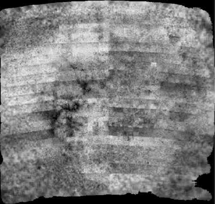
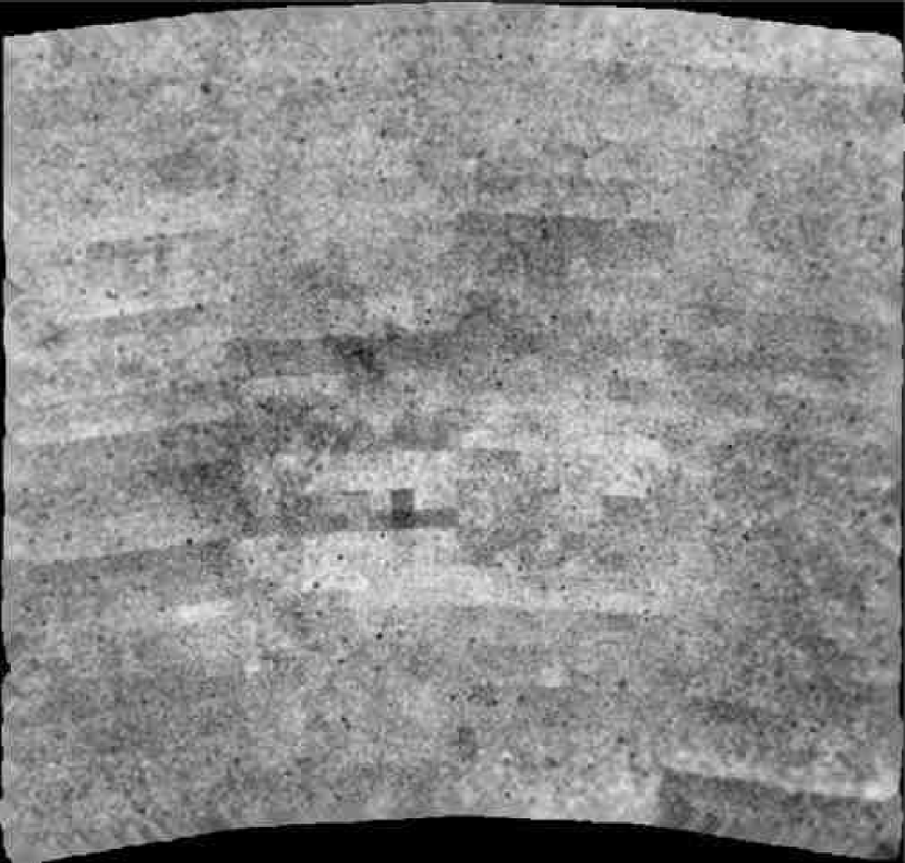
Figure 8.— The spatial map of extinction values as derived for both the cooler, older stars ($5500{\ \rm K}\leq T_{E}\leq 6500{\ \rm K}$ ; right panel) and the hotter, younger stars ($12000{\ \rm K}\leq T_{E}\leq 45000{\ \rm K}$; left panel) for the entire survey region. The small localized circular regions of apparent high extinction are globular clusters, which have some anomalous photometry because of their high stellar densities. Sharp spatial variations are due to scan-to-scan photometry differences of a few hundredths of a magnitude.

In Figure  8 we show the spatial distribution of line-of-sight extinction derived from both the hot and cold stellar populations. Because the recovery of A_V is quite sensitive to color, subtle differences in the scan photometry are highlighted in the extinction maps. For example, a set of small photometric differences (0.03 mag in opposite senses in $B$ and $I$, so that $B-I$ has changed by 0.06 mag) creates an extinction discontinuity of the magnitude observed at many scan edges in the hot population map of Figure  8.

The principal coherent extinction structure within the LMC is the increase in extinction in the hot star population along the north-east ridge of the LMC bar. This structure is also visible in the map from the colder stars. As expected, the increased extinction correlates with sites of star formation that can be seen in the stellar density images (Figure  2), in 100$\mu$m images (Wheelock et al., 1991), and in CO maps (Fukui et al., 1999).

The A_V histograms of the two populations are shown in Figure 9. As we found for a small region of the LMC (Zaritsky, 1999), the mean extinction is lower for the cooler populations (average A_V’s of 0.43 mag vs 0.55 mag for the cold vs. hot population, respectively). The bimodal distribution of extinction values among the cooler stars is characteristic of a geometry where the stars are distributed in front and behind a thinner mid-plane dust plane (see Figure 12 of Harris et al. (1997)). The lack of such bimodaility in the $A_{V}$ distribution of the hotter stars suggests that those are distributed within the dust layer. This geometric model is further supported by the correspondence between the $A_{V}$ values of the maximum in the hot star $A_{V}$ distribution and the local minimum in the cold star $A_{V}$ distribution.

3.1. A Simple Model

To explore the dependence of the $A_{V}$ distribution on the relative distributions of the dust and stars, we develop a simple geometrical model. We construct a galaxy using three components: a “cold” star component that matches the projected spatial distribution of such stars, a “hot” star component that matches the projected spatial distribution of such stars, and a dust layer that corresponds to the dust map developed from the “hot” stars plus additional components for a diffuse, homogeneous internal dust layer and Galactic foreground, which is estimated to be minimal ($A_{V}\sim 0.05$). The two dust components associated with the LMC, a clumped component seen in the extinction map and a possible smooth component that is not as easily detected, are defined to have the same vertical scale height. We then randomly place “cold” stars along the line of sight, but spatially constrain them to follow the observed distribution by placing them at the same $(\alpha,\delta)$ as each observed “cold” star. Each star is reddended according to the local value of $A_{V}$ (taken to reflect the midplane value of extinction as derived from the hot stars) and its position relative to the dust layer (for example, stars in front of the disk layer are extincted only by the Galactic foreground component, while stars behind the dust layer are extincted by twice the measured value of $A_{V}$ plus the hypothesized diffuse layer.

Figure 9.— The distribution of extinction values for the two stellar populations and a simple model. We show the distribution of $A_{V}$ for the hotter stellar population (upper panel) and for the colder stellar population (lower panel), where the solid and dotted line represent the unadjusted and adjusted $U$-band photometry. The dashed line in the lower panel represents the expected distribution of $A_{V}$ for an older stellar populations derived from the simple model detailed in the text. The sharp rise at zero extinction is due to observational uncertainties that scatter measurements to negative $A_{V}$, which we set to $A_{V}=0$. The model shows the same rise at $A_{V}=0$.

We explore a range of relative thicknesses of the star and dust layers, and of the optical depth of the diffuse layer. A model that reproduces the salient features of the distribution of $A_{V}$ for the cold population is shown in Figure 9. The particular model shown has a scaleheight for the cold stars that is ten times that of the dust, a Gaussian distributed error in the measured $A_{V}$ of 0.125 mag, an optical depth for the diffuse layer, $\tau_{f}$, of 0.28 (if the optical depth as estimated by the young stars in a region is $<$ 0.28, we set the value to 0.28), and a foreground extinction optical depth of 0.05, which sets the position of the peak of the low-$A_{V}$ population. The model excellently reproduces the $A_{V}$ distribution for $A_{V}<0.7$ and underestimates $A_{V}$ for larger values. It may therefore be the case that there are pockets of higher optical depth in the midplane than modeled or a radial dependence in the extinction of the diffuse component that perhaps increases toward the LMC center, but adding those in an ad hoc manner to the models introduces far too many free parameters. Because of this systematic issue, we do not provide “best-fit” values for the parameters of our model, but instead simply show one satisfactory example.

Figure 10.— A comparison of the distribution of extinction values for the older stellar population and models. The histogram shows the data, the solid curve shows the model shown in Figure 9, the short-dashed line represents the $\tau_{f}=0.4$ model, the long-dashed line represents the model with a stellar scaleheight that is 5 times that of the dust layer, the dot-dahsed line represents the exponentially declining $\tau_{f}$ model.

There is some degeneracy between the various parameters, but large deviations from the values quoted above produce qualitatively inferior fits. For example, modifying $\tau_{f}$ to correspond to $A_{V}=0.4$ produces a highly inferior fit (Figure 10) and decreasing the stellar scaleheight by a factor of two fills in the valley between the two peaks of extinction values. An interesting variant of the model is to presume that $\tau_{f}$ has a radial dependence. If $\tau_{f}$ decreases exponentially with increasing radius, we find that for small values of the scalelength (for example, a 1 kpc scalelength for the model shown in Figure 10), the second peak is diluted, due to the spread in midplane extinction values in such a model, but that we do better at reproducing the high end tail of the extinction distribution because we can drive the extinction at the center of disk high and not affect large numbers of stars. Of course there are other solutions to the high-end extinction distribution, so this agreement alone does not argue for the model with exponentially declining $\tau_{f}$. Models with large scalelengths approach the uniform $\tau_{f}$ model, while models with smaller scalelengths further dilute the second peak.

While the distribution of dust is undoubtedly more complicated than the description adopted in these models, the models are able to reproduce the peak at $A_{V}=0$, the peak at $A_{V}\sim 0.05$, the bimodal peak distribution, the position of the second peak, and the tail toward high $A_{V}$ values with fairly minimal model assumptions. This suggests that as a global average the model is qualitatively correct. Even so, it is a much more complicated description of the internal absorption in galaxies than generally adopted. Some studies that focus on internal extinction (Witt, Thronson, & Capuano, 1992; Misselt et al., 2001) explicitly deal with the distributions of stars and dust, but the general default correction is based on a foreground sheet assumption and an effective extinction curve. Because of the partial correlation of dust with star formation, this effective extinction curve is likely to be highly complex, dependent on geometry, and sensitive to the evolutionary state of the system.

4. Summary

We have conducted a broad-band photometric survey of the Magellanic Clouds. We present the data for over 24 million stars in the $8.5^{\circ}\times 7.5^{\circ}$ survey area centered on the Large Magellanic Cloud. The catalog contains positions (right ascension and declination in J2000 coordinates) and $U$, $B$, $V$, and $I$ magnitudes and uncertainties in the Johnson-Kron-Cousins photometric system measured from our drift scan images.

Using this catalog, we have constructed extinction maps for two stellar populations in the LMC. We find 1) that this dust is highly localized near the younger, hotter stars, and in particular toward regions immediately east and northeast of the center of the LMC, 2) that aside from these regions of higher extinction, there is no discernible global pattern, 3) that on average the extinction toward the younger, hotter stars is only about 0.1 mag larger, but that the distributions of extinctions are entirely different, 4) that the distribution of extinctions along lines-of-sight toward the older stars is bimodal, and 5) that the bimodial $A_{V}$ distribution is easily modeled as stars in front and behind a thinner dust layer. The two external galaxies for which we now have highly detailed maps of extinction as a function of stellar population both show significant differences in the extinction toward those populations. This difference, or at least the potential for this difference, should be considered when correcting the photometry of other galaxies for internal extinction.

ACKNOWLEDGMENTS: DZ acknowledges financial support from an NSF grants (AST-9619576 and AST-0307482), a NASA LTSA grant (NAG-5-3501), and fellowships from the David and Lucile Packard Foundation and the Alfred P. Sloan Foundation. EKG acknowledges support from NASA through grant HF-01108.01-98A from the Space Telescope Science Institute and from the Swiss National Science Foundation through grant 200021-101924/1.

References

- Cioni et al. (2000) Cioni, M-R., et al., 2000, A&AS, 144, 235
- Fukui et al. (1999) Fukui, Y. et al. 1999, PASJ, 51, 745
- Gordon et al. (2003) Gordon, K. D., Clayton, G. C., Misselt, K. A., Landolt, A.U., & Wolff, M. J. 2003, ApJ, 594, 279
- Grebel & Roberts (1995) Grebel, E.K., & Roberts, W. J. 1995, A&AS, 109, 293
- Harris & Zaritsky (2003) Harris, J. & Zaritsky, D., 2003 AJ, 127, 1531
- Harris et al. (1997) Harris, J., Zaritsky, D., & Thompson, I 1997 AJ, 114, 1933
- Landolt (1983) Landolt, A.U. 1983, AJ, 88, 439
- Landolt (1992) Landolt, A.U. 1992, AJ, 104, 340
- Lejeune et al (1997) Lejeune, Th., Cuisinier, F., & Buser, R. 1997, A&AS, 125, 229
- Massey (2002) Massey, P. 2002, ApJS, 141, 81
- Misselt et al. (2001) Misselt, K.A., Gordon, K. D., Clayton, G. C., and Wolff, M. J. 2001, ApJ, 551, 277
- Schild (1977) Schild, R. E. 1977, AJ, 82, 337
- Stetson (1987) Stetson, P. 1987, PASP, 99, 191
- Tucholke et al. (1996) Tucholke, H.-J., de Boer, K. S., & Seitter, W.C. 1996, A&A, 119, 91
- van der Marel & Cioni (2001) van der Marel, R.P., 2001, AJ, 122, 1807
- Wheelock et al. (1991) Wheelock, S. L. et al. 1991, IRAS Sky Survey Atlas Explanatory Supplement
- Witt, Thronson, & Capuano (1992) Witt, A. N., Thronson, H.A., Jr., & Capuano, J.M., Jr. 1992, ApJ, 393, 611
- Zaritsky (1999) Zaritsky, D., 1999, AJ, 195, 6801
- Zaritsky et al. (1997) Zaritsky, D., Harris, J., & Thompson, I. 1997, AJ, 114, 1002
- Zaritsky et al. (1996) Zaritsky, D., Shectman, S.A., & Bredthauer, G 1996, PASP, 108, 104
- Zaritsky et al. (2000) Zaritsky, D., Harris, J., Grebel, E.K., & Thompson, I. 2000, ApJ, 534, 53
- Zaritsky et al. (2002) Zaritsky, D., Harris, J., Thompson, I.B., Grebel, E.K., & Massey, P. 2002, AJ, 123, 855