Metal abundances in extremely distant Galactic old open clusters.
I. Berkeley 29 and Saurer 1¹

Abstract

We report on high resolution spectroscopy of four giant stars in the Galactic old open clusters Berkeley 29 and Saurer 1 obtained with HIRES at the Keck telescope. These two clusters possess the largest galactocentric distances insofar known for open star clusters, and therefore are crucial objects to probe the chemical pattern and evolution of the outskirts of the Galactic disk. We find that $[Fe/H]=-0.38\pm 0.14$ and $[Fe/H]=-0.44\pm 0.18$ for Saurer 1 and Berkeley 29, respectively. Based on these data, we first revise the fundamental parameters of the clusters, and then discuss them in the context of the Galactic disk radial abundance gradients. Both clusters seem to significantly deviate from the general trend, suggesting that the outer part of the Galactic disk underwent a completely different evolution compared to the inner disk. In particular Berkeley 29 is clearly associated with the Monoceros stream, while Saurer 1 exhibits very different properties. The abundance ratios suggest that the chemical evolution of the outer disk was dominated by the Galactic halo.

1 Introduction

The detailed knowledge of the present day Galactic disk abundance gradient and its evolution with time is one of the basic ingredients of any chemical evolution model which aims to predict the properties of the Galactic disk (Matteucci 2004 and references therein). Compared to other indicators (HII regions, B stars, planetary nebulae and Cepheids), old open clusters (OCs) present the advantage of both sampling almost the entire disk and covering basically all of the history of the disk from its infancy to now. In recent years, renewed efforts to probe the chemical abundances in old OCs have taken place, by means of high resolution spectroscopy of member stars (Friel et al., 2003; Bragaglia et al., 2001; Peterson & Green, 1998; Carretta et al., 2004). In fact, the Galactic disk radial abundance gradients (Friel & Janes, 1993; Carraro et al., 1998; Friel et al., 2002) mostly rely on medium resolution spectra, and the derived metallicities turned out to be quite different in several cases when high resolution spectra are available (see, e.g., Carretta et al. 2004).
An additional drawback stems from the fact that it is quite common to consider the radial abundance gradient observed in the solar vicinity as representative of the whole disk, due to the lack of metallicity estimates in very distant OCs. It is therefore highly desirable to obtain information on the chemical compositions of old OCs spanning the widest possible range in galactocentric distances, covering in particular the relatively unexplored outer disk of the Galaxy.

In this paper we present high resolution spectra of four giant stars in the old OCs Berkeley 29 and Saurer 1. According to Kaluzny (1994) and Carraro & Baume (2003) these two objects are the most distant OCs insofar detected in the Milky Way (beyond 19 kpcs from the Galactic center), although the precise distances are not yet very well known, due to uncertainties in the reddening and metallicity. In fact only photometric estimates of the metallicity are available for these clusters, which are based mainly on isochrone fitting or comparison with other oprn clusters. Kaluzny (1994) reports for Berkeley 29 an age of 4 Gyrs and and the very low metal content $[Fe/H]\approx-1.0$, while Carraro & Baume (2003) report for Saurer 1 an age of 5 Gyrs and a metal content $[Fe/H]\approx-0.5$ Thus, they represent very useful targets to probe the metal abundance of the Galactic disk outskirts, allowing us to significantly enlarge the distance baseline of the radial abundance gradient. Here we present new metallicity estimates for the two clusters and derive updated estimates of their age and distance, and discuss their role in shaping the radial abundance gradient.
The layout of the paper is as follows. Section 2 and 3 illustrate observations and reduction strategies, while Section 4 deals with radial velocity determinations. In Section 5 we derive the stellar abundances and in Section 6 we revise the cluster fundamental parameters. The results of this paper are then discussed in Section 7 and, finally, summarized in Section 8.

2 Observations

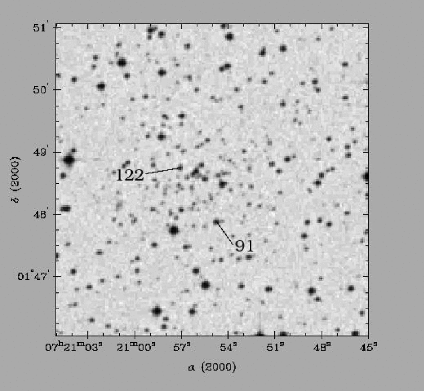
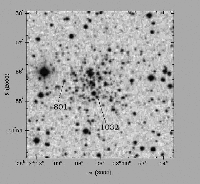
Figure 1: Digital Sky Survey (DSS) finding charts of the observed stars in Berkeley 29 (right panel) and Saurer 1 (left panel)

The observations were carried out on the night of January 14, 2004 at the W.M. Keck Observatory under photometric conditions and typical seeing of 1″. The HIRES spectrograph (Vogt et al., 1994) on the Keck I telescope was used with a 1.15 x 7 arcsec slit to provide a spectral resolution R = 34,000 in the wavelength range 5720$--$8160 Å in 19 different orders on the 2048$\times$2048 CCD detector. A blocking filter was used to remove second$-$order contamination from blue wavelengths. Three exposures of 2400 seconds were obtained for the two stars in Berkeley 29. For Saurer 1$-$91 and Saurer 1$-$122 we took two exposures of 3000 and 2700 seconds, respectively. For the wavelength calibration, spectra of a thorium$-$argon lamp were secured after the set of exposures for each star was completed. The radial velocity standard HD 26162 was observed at the beginning of the night, together with the spectrophotometric standard G191B2B.
In Fig. 1 we show a finding chart for the two clusters where the four observed stars are indicated, while in Fig. 2 we show the position of the stars in the Color$-$Magnitude Diagram (CMD).

3 Data Reduction

Images were reduced using IRAF, including bias subtraction, flat$-$field correction, extraction of spectral orders, wavelength and flux calibration, and continuum subtraction. The single orders were merged into a single spectrum and the spectra of each star were combined to remove cosmic rays. A spectral region containing a large number of telluric lines was instead used to correct the spectra for flexures of the instrument and off$-$center slit pointing; the error on this correction was about 0.05 km s^-1. An example of sprectrum, with a few line indicated, is shown in Fig. 3.

4 Radial Velocities

No radial velocity estimates are available for Berkeley 29 and Saurer 1. The radial velocities of the target stars were measured using the IRAF FXCOR task, which cross$-$correlates the object spectrum with the template (HD 26162); the peak of the cross$-$correlation was fitted with a gaussian curve after rejecting spectral regions contaminated by telluric lines ($\lambda>6850$ Å). In order to check our wavelength calibration we also measured the radial velocity of HD 26162 itself, using the Doppler shifts of various spectral lines. We obtained a radial velocity of 24.8$\pm$0.1 km s^-1, which perfectly matches the catalogue value (24.8 km/sec, Wielen et al. 1999). The final error in the radial velocities was typically about 0.1 km s^-1. The two stars we measured in each clusters have compatible radial velocities (see Table 1), and are considered, therefore, bona fide cluster members.

5 ABUNDANCE ANALYSIS

5.1 Atomic parameters and equivalent widths

We derived equivalent widths of spectral lines by using the interactive software SUPERSPECTRE (freely distributed by Chris Sneden, University of Texas, Austin). This software has the advantage of providing a graphical visualisation of the continuum and of the measured width. Repeated measurements show a typical error of about 4$-$5 mÅ, also for the weakest lines. We checked the equivalent widths derived from SUPERSPECTRE by measuring them also using standard IRAF routine SPLOT, and found a fair agreement, with maximum differences amounting to 5mÅ. The line list (FeI, FeII, Mg, Si, Ca, Al,, Na, Ni and Ti, see Table 3) was taken from Friel et al. (2003), who considered only lines with equivalent widths narrower than 150mÅ, in order to avoid non$-$linear effects in the LTE analysis of the spectral features. Oxygen lines were taken from Cavallo et al. (1997). We are aware that the use of high excitation O triplet lines is controversial. Most problems however arise in metal poor stars ($[Fe/H]\leq 1$) and for temperatures larger than 6200 ${}^{0}K$ (King & Boesgaard 1995). Our stars are metal richer than this value and cooler, a fact which makes us confident about the derivation of the O abundance .

5.2 Atmospheric parameters

Initial estimates of the atmospheric parameter $T_{eff}$ were obtained from photometric observations in the optical (BVI) and infrared (JHK) from 2MASS. VI data were available for Saurer 1 (Carraro & Baume, 2003) and BV for Berkeley 29 (Kaluzny, 1994). Reddening values are E(V$-$I)= 0.18 and E(B$-$V)= 0.21, respectively. First guess effective temperatures were derived from the (V$-$I)–$T_{eff}$ and (B$-$V)–$T_{eff}$ relations, the former from Alonso et al. (1999) an the latter from Gratton et al. (1996). We then adjusted the effective temperature by minimizing the slope of the abundances obtained from Fe I lines with respect to the excitation potential in the curve of growth analysis. While in the case of Saurer 1 the derived temperature yields a reddening consistent with the photometric one, in the case of Berkeley 29 the spectroscopic reddening turns out to be E(B$-$V)= 0.08, significantly smaller than the photometric one (see the discussion in Sect 6).
Initial guesses for the gravity $\log$(g) were derived from:

$$log(\frac{g}{g_{\odot}})=log(\frac{M}{M_{\odot}})+4\times log(\frac{T_{eff}}{T_{\odot}})-log(\frac{L}{L_{\odot}})$$ (1)

taken from Carretta & Gratton (1997). In this equation the mass $\frac{M}{M_{\odot}}$ was derived from the comparison between the position of the star in the Hertzsprung$-$Russell diagram and the Padova Isochrones (Girardi et al., 2000). The luminosity $\frac{L}{L_{\odot}}$ was derived from the the absolute magnitude $M_{V}$, assuming the literature distance moduli of 15.8 for Berkeley 29 (Kaluzny, 1994) and 16.0 for Saurer 1 (Carraro & Baume, 2003). The bolometric correction (BC) was derived from the relation BC–$T_{eff}$ from Alonso et al. (1999). The input $\log$(g) values were then adjusted in order to satisfy the ionization equilibrium of Fe I and Fe II during the abundance analysis. Finally, the micro$-$turbulence velocity is given by the following relation (Gratton et al., 1996):

$$v_{t}[kms^{-1}]=1.19\times 10^{-3}\times T_{eff}-0.90\times log(g)-2$$ (2)

The final adopted parameters are listed in Table 2.

5.3 Abundance determination

The LTE abundance program MOOG (freely distributed by Chris Sneden, University of Texas, Austin) was used to determine the metal abundances. Model atmospheres were interpolated from the grid of Kurucz models (1992) by using the values of $T_{eff}$ and $\log$(g) determined as explained in the previous section. During the abundance analysis $T_{eff}$, $\log$(g) and $v_{t}$ were adjusted to remove trends in excitation potential, ionization equilibrium and equivalent width for Fe I and Fe II lines. Table 3 contains the atomic parameters and equivalent widths for the lines used. The first column is the name of the element, the second the wavelength in Å, the third the excitation potential, the fourth the oscillator strength $\log$ (gf), and the remaining ones the equivalent widths of the lines for the observed stars.
The derived abundances are listed in Table 4, together with their uncertainties. The measured iron abundances are [Fe/H]=-0.38$\pm 0.14$ and [Fe/H]=-0.44$\pm 0.18$ for Saurer 1 and Berkeley 29, respectively. The reported errors are derived from the uncertainties on the single star abundance determination (see Table 4) Somewhat surprisingly, we do not find extremely low metal abundances, as one would expect from the large galactocentric distances and the known abundance gradient (Friel et al., 2002).

As a check for the entire procedure, we derived the abundances for the star Arcturus (Friel et al. 2003) following the same recipe as for the main targets, and obtaining abundance values well consistent with the values reported by Friel et al. 2003, who performed the same kind of analysis. The results have been listed in Tables 4 and 5.

Finally, following the method described in Villanova et al. (2004), we derived the stellar spectral classification, which we provide in Table 1.

6 REVISION OF CLUSTER PROPERTIES

Our study is the first to provide spectral abundance determinations of stars in Berkeley 29 and Saurer 1. Here we briefly discuss the revision of the properties of these two clusters which follow from our measured chemical abundances.

6.1 Saurer 1

Saurer 1 was recently studied by Carraro & Baume (2003), who, on the basis of deep VI photometry and a comparison with stellar models, derived and age of 5 Gyr, a distance of 19.2 kpc and a reddening E(V$-$I)=0.18. These authors suggest that the probable metal content of the cluster is around Z=0.008. Here we obtained [Fe/H]=$-$0.38$\pm$0.14, which corresponds to Z=0.007, thus confirming the photometric estimate. By using the new metallicity, then, the cluster properties are not modified in a significant way. We confirm both the photometric reddening and the Galactocentric distance derived by Carraro & Baume (2003).

6.2 Berkeley 29

Berkeley 29 was studied by Kaluzny (1994), who suggested a reddening E(B$-$V)=0.21 and a very low metallicity of about [Fe/H]=$-$1.0. By assuming these values, Kaluzny (1994) derived a Galactocentric distance of 18.7 kpc. The present study provides different results. In fact, the spectroscopic reddening turns out to be E(B$-$V)=0.08, significantly lower than the Kaluzny estimate, and the metallicity [Fe/H]=$-$0.44$\pm$0.18, significantly higher. These new values of reddening and metallicity yield new age and galactocentric distance estimates, 4.5 Gyr and 21.6 kpc, respectively. These estimates have been obtained by comparing the cluster CMD with the exact metallicity isochrones from (Girardi et al., 2000). Therefore Berkeley 29 is the most distant open cluster in the Milky Way currently known.

7 THE RADIAL ABUNDANCE GRADIENT

In Fig. 4 we plot the radial abundance gradient as derived from Friel et al. (2002), which is at present the most updated version of the gradient itself.
The clusters included in their work (open squares) define an overall slope of $-$0.06$\pm$0.01 dex kpc^-1 (solid line). For the sake of the simplicity, we assume for the moment that the two new clusters analyzed in the present work $-$Saurer 1 and Berkeley 29$-$ are two genuine Galactic disk old OCs. They (filled circles) clearly deviate from the general trend. However, if we take them into account, the slope of the gradient would be much flatter, i.e. $-$0.03$\pm$0.01 dex kpc^-1.
The same conclusion could be extended to the age$-$dependent radial abundance gradient. Friel et al. (2002) used 39 clusters to show that the radial abundance gradient becomes flatter with time (see their Fig. 3), although one has to note that different age gradients have different spatial baselines and therefore describe different zones of the disk. This result contrasts with the previous analysis by Carraro et al. (1998), where no trend was found with age in a sample of similar size (37 clusters), except for a slight steepening of the gradient at intermediate ages (see their Fig. 7). When adding the two new clusters, Berkeley 29 and Saurer 1, the radial gradient in the older bin becomes almost completely flat. In addition we note that if one adds the new [Fe/H] determinations for NGC 2506, IC 4651 and NGC 6134 by Carretta et al. (2004), the gradient disappears almost completely also in the younger age bin, thus confirming the overall trend proposed by Carraro et al. (1998).

8 ABUNDANCE RATIOS

Friel et al. (2003) discussed the trends of abundance ratios for old open clusters and concluded that all the old OCs for which abundance ratios are available show scaled solar abundance ratios, with no correlation with overall cluster [Fe/H] or with cluster age. The only deviation from this conclusion was found in Collinder 261, a 8 Gyr cluster, where Si and Na abundances are slightly enhanced. The same trend for these two elements is reported by Bragaglia et al. (2001) for NGC 6819, a 3 Gyr open cluster with higher than solar metal abundance. Apart from these two elements, however, old OCs show scaled solar abundances, in agreement with typical Galactic disk field stars.

In Table 5 we list the abundance ratios for the observed stars in Berkeley 29 and Saurer 1. Our program clusters have ages around 5 Gyrs and iron metal content [Fe/H] $\approx$ $-$0.4. They are therefore easily comparable with clusters having similar properties discussed earlier in the literature, such as NGC 2243 and Melotte 66 (see Friel et al. 2003, Tab. 7). It is interesting to note that while the latter two clusters have scaled solar abundances, our program clusters have generally enhanced values for all the abundance ratios.

At a similar [Fe/H], Berkeley 29 and NGC 2243 have different values for all the abundance ratios, with the exception of [Mg/Fe], although the average [$\alpha$/Fe] ratio is enhanced in Berkeley 29 and solar scaled in NGC 2243. Berkeley 29 also exhibits enhanced [O/Fe] with respect to NGC 2243.

The same conclusions can be drawn for Saurer 1, when compared with Melotte 66, an old open cluster of similar age and [Fe/H]. All the abundance ratios in Saurer 1 appear enhanced when compared with Melotte 66, except for [O/Fe], which is similar in the two clusters.

9 DISCUSSION

By looking at Fig. 4 one can argue that fitting with a straight line all the data points does not have any statistical meaning. Simply, the two new points (filled circles) deviate from the bulk of the other points.
These results seem instead to imply that the chemical properties of the outer galactic disk are different from the bulk of the disk itself. We propose here two possible explanations:

1) In a series of papers (Crane et al. 2003; Frinchaboy et al. 2003; Rocha-Pinto et al. 2003), it has been shown that a ring$-$like stellar structure, the Monoceros stream, exists in the direction of the Galactic anticenter, which could represent the debris of a disrupting dwarf galaxy in a noncircular, prograde orbit around the Milky Way. In particular, Frinchaboy et al. (2003) proposed that a number of globular and old OCs might be associated with the stream. With a radial velocity of 24.6$\pm$0.1 km s^-1 and a galactic longitude of 197$\fdg$98, Berkeley 29 seems to be well associated with the stream (see Fig. 2 in Frinchaboy et al. 2003). Moreover, its metallicity of [Fe/H]=$-$0.44$\pm$0.18 perfectly matches the global metal abundance of the stream ($-$0.4$\pm 0.3$).
We cannot, however, draw the same conclusion for Saurer 1. Although the metal abundance is the right one, the longitude 214$\fdg$31 and the radial velocity of 104.6$\pm$0.1 km s^-1 completely rule out the possibility that this cluster is associated with the stream. One should invoke another explanation to justify the particular location of this cluster in the Galactic disk radial abundance gradient.

2) Some Galactic chemical evolution models predict that the chemical evolution of the outer disk is dominated by the halo, and therefore it undergoes a completely different evolution from the bulk of the disk. We took the radial abundance gradient predicted by the C-model of Chiappini et al. (2001), which assumes that the Milky Way formed through two main collapse events, the first one generating the halo and the bulge, the second one smoothly building up the disk inside$-$out. In this model, a higher initial enrichment due to star formation in the halo is reached in the outer thin disk. This is due to the fact that, although halo and disk formed almost independently, the halo gas is predominating in the outermost disk regions and it creates a pre$-$enriched disk gas dominating the subsequently accreted primordial one. This gives origin to the rise in [Fe/H] at large galactocentric distances (see Fig. 4, dotted line). At smaller galactocentric distances, the amount of disk gas always predominates, thus diluting the enriched halo gas which falls onto it. We finally recall that the negative abundance gradient predicted for galactocentric distances smaller than 15$-$16 kpc is due, in this framework, to the assumption of an inside$-$out formation of the galactic thin disk. In Fig 4 we show the expected behaviour of the gradient in the outskirts of the disk, and an inversion of the slope is predicted to occur at 13$-$14 kpc from the Galactic center, roughly as observed. We stress that chemical evolution models simply rely on abundances and abundance ratios, and cannot take into account the kinematics of the stellar population. However, the agreement between model and observations is rather striking. Further support to this scenario comes from the analysis of the expected abundance ratios in the outskirts of the disk. Here the models by Chiappini et al. (2001) predict overabundances in O and $\alpha$ elements similar to what we actually observe, due to the fact that the model evolution is dominated by the old stellar population of the Galactic halo.

It is true that our results rely on four stars in two clusters, and that more data are needed to clarify the global issue of the evolution of the outer Galactic disk. However it is quite clear from the present analysis the the outer disk does not reflect the general trend seen in the inner disk, and that the outer disk is probably the outcome a series of mergers occured in the past, in the same fashion as the Galactic halo.

10 CONCLUSIONS

We have presented high resolution spectroscopy of four giant stars in the extremely distant old OCs Saurer 1 and Berkeley 29, and provided the first estimate of their metal abundances. We have found that these two clusters do not belong to the old open cluster family of the Milky Way, since they significantly deviate from the global radial abundance gradient and exhibit abundance ratios typical of the Galactic halo rather than the Galactic disk. Moreover they are located quite high onto the Galactic plane, a position which better fits into the thick disk of the Galaxy.
Berkeley 29 is presumably associated with the Monoceros stream, whereas Saurer 1 does not belong at all to the stream, and shows quite different kinematic features. Without taking the kinematics into account, the anomalous behaviour of these two clusters can be explained by assuming that the outer parts of the disk evolved in a different way with respect to the bulk of the disk itself, and that the chemical evolution driver at those distances was the Galactic halo (Chiappini et al., 2001). In fact the abundance ratios, in particular [O/Fe] and [$\alpha$/Fe], show the typical enhancements expected in an old stellar population like the Milky Way halo.

Figure 2: Position of the observed stars in the CMD of Saurer 1 (left panel, photometry from Carraro & Baume 2003) and Berkeley 29 (right panel, photometry from Kaluzny 1994).

Figure 3: An example of extracted spectrum for the star Be 29-801, with the main lines indicated

Figure 4: The Galactic disk chemical abundance radial gradient. Open quares are data from Friel et al. (2002), whereas filled circles are Berkeley 29 and Saurer 1 (this work). The solid line is the linear fit to the Friel et al. (2002) data, whereas the dashed line is a linear fit to all the data points. The dotted line is the radial gradient behavior expected from a chemical evolution model (Chiappini et al. 2001).

Table 1: OBSERVED STARS

ID	RA	DEC	V	(V$-$I)	$V_{rad}$ (km s-1)	$S/N$	Spectral Type	comments
Sau 1-91	07:20:54.75	+01:47:53.09	16.43	1.11	+104.4$\pm$0.1	80	G7III	Carraro & Baume (2003)
Sau 1-122	07:20:57.08	+01:48:44.97	16.92	1.17	+104.8$\pm$0.1	80	G9III	Carraro & Baume (2003)
Be 29-801	06:53:08.07	+16:55:40.53	16.58	1.06	+24.5$\pm$0.1	70	G6III	Kaluzny (1994)
Be 29-1032	06:53:03.50	+16:55:08.50	16.56	1.05	+24.8$\pm$0.1	70	G6III	Kaluzny (1994)

Table 2: ADOPTED ATMOSPHERIC PARAMETERS

ID	Teff(K)	log g (dex)	$v_{t}$ (km s-1)
Sau 1-91	5070$\pm$50	2.8$\pm$0.1	1.60
Sau 1-122	4900$\pm$50	2.6$\pm$0.1	1.50
Be 29-801	5090$\pm$50	2.6$\pm$0.1	1.70
Be 29-1032	5070$\pm$50	2.6$\pm$0.1	1.70

Table 3: EQUIVALENT WIDTHS

Element	$\lambda(\AA)$	$E.P.$	$log\;{\it gf}$	$Sa1-91$	$Sa1-122$	$Be29-801$	$Be29-1032$
Fe I	5753.120	4.240	-0.92	86.7	71.5	78.8	99.1
Fe I	5775.081	4.220	-1.31	68.5	66.8	62.4	67.5
Fe I	6024.058	4.548	+0.16	105.0	117.0	109.0	106.7
Fe I	6042.226	4.652	-0.89	60.9	$\cdots$	58.9	60.5
Fe I	6082.72	2.22	-3.65	56.9	64.7	66.1	-
Fe I	6151.620	2.180	-3.27	74.6	94.0	72.0	77.2
Fe I	6165.360	4.143	-1.58	53.0	63.5	51.7	43.2
Fe I	6173.340	2.220	-2.89	98.1	105.0	80.5	84.0
Fe I	6229.230	2.845	-3.04	45.2	74.7	55.5	54.2
Fe I	6246.320	3.590	-1.00	127.1	130.9	112.7	117.3
Fe I	6344.15	2.43	-2.97	86.9	109.4	90.2	95.7
Fe I	6481.880	2.280	-2.90	104.3	102.6	86.5	90.8
Fe I	6574.229	0.990	-5.00	44.1	79.9	71.8	74.3
Fe I	6609.120	2.560	-2.44	98.8	$\cdots$	94.1	93.7
Fe I	6703.570	2.758	-3.08	53.9	55.6	51.7	53.3
Fe I	6705.103	4.607	-1.17	55.9	66.0	45.3	44.1
Fe I	6820.372	4.638	-1.05	55.1	48.8	43.2	43.1
Fe I	6839.831	2.559	-3.48	$\cdots$	$\cdots$	51.3	57.9
Fe I	7461.520	2.560	-3.64	52.1	60.9	61.4	56.4
Fe I	7568.900	4.280	-0.93	102.7	94.4	75.2	80.4
Fe I	7723.200	2.280	-3.51	79.9	91.9	61.9	-
Fe I	7807.909	4.990	-0.66	$\cdots$	$\cdots$	51.0	57.9
Fe II	6084.100	3.20	-3.95	35.2	$\cdots$	33.0	27.9
Fe II	6149.250	3.89	-2.81	44.4	45.8	47.0	56.2
Fe II	6247.560	3.89	-2.65	55.2	56.9	56.8	65.8
Fe II	6369.463	2.89	-4.22	$\cdots$	$\cdots$	30.9	-
Fe II	6416.930	3.89	-2.67	58.0	53.2	51.1	36.0
Fe II	6456.390	3.90	-2.35	$\cdots$	66.4	71.5	79.0
Fe II	6516.080	2.89	-3.34	72.2	72.9	76.2	85.5
Al I	6696.03	3.14	-1.44	$\cdots$	$\cdots$	34.4	-
Al I	6698.67	3.13	-1.94	32.4	35.5	28.9	24.0
Ca I	6161.30	2.52	-1.07	83.0	92.1	72.3	75.3
Ca I	6166.44	2.52	-1.17	$\cdots$	97.4	80.9	70.9
Ca I	6455.60	2.52	-1.44	72.5	81.5	72.1	58.0
Ca I	6499.65	2.52	-0.93	107.3	119.9	101.2	103.2
Mg I	7387.70	5.75	-1.00	62.8	69.5	58.7	50.0
Na I	6154.23	2.10	-1.80	50.1	48.0	42.8	32.2
Na I	6160.75	2.10	-1.58	73.2	73.5	64.0	59.9
Ni I	6175.37	4.09	-0.68	57.6	74.9	60.2	48.0
Ni I	6176.81	4.09	-0.22	83.8	86.1	72.5	68.4
Ni I	6223.99	4.10	-1.11	$\cdots$	42.1	33.0	35.0
Si I	5793.08	4.93	-2.11	$\cdots$	48.1	48.2	37.5
Si I	6142.49	5.62	-1.86	37.6	$\cdots$	14.1	14.0
Si I	6145.02	5.61	-1.56	$\cdots$	45.4	34.7	39.7
Si I	6243.82	5.61	-1.48	54.5	50.6	54.3	43.3
Si I	7034.91	5.87	-0.95	$\cdots$	$\cdots$	49.8	59.4
Ti I	5978.54	1.87	-0.52	41.5	65.4	36.5	39.8
O I	7771.95	9.14	+0.28	61.0	55.0	38.0	45.3
O I	7774.18	9.14	+0.15	51.0	37.4	50.6	33.9
O I	7775.39	9.14	-0.14	40.3	20.1	30.3	32.1

Table 4: MEAN STELLAR ABUNDANCES

ID	[FeI/H]	[FeII/H]	[AlI/H]	[CaI/H]	[MgI/H]	[NaI/H]	[NiI/H]	[SiI/H]	[TiI/H]	[OI/H]
Sau 1-91	-0.38$\pm$0.14	-0.41$\pm$0.07	-0.03$\pm$0.15	-0.22$\pm$0.15	-0.37$\pm$0.10	+0.10$\pm$0.15	-0.23$\pm$0.10	+0.10$\pm$0.15	-0.37$\pm$0.15	+0.11$\pm$0.15
Sau 1-122	-0.38$\pm$0.15	-0.41$\pm$0.05	-0.07$\pm$0.15	-0.15$\pm$0.16	-0.33$\pm$0.10	-0.01$\pm$0.15	-0.14$\pm$0.11	-0.10$\pm$0.14	-0.14$\pm$0.15	-0.04$\pm$0.15
Be 29-801	-0.45$\pm$0.16	-0.53$\pm$0.10	-0.27$\pm$0.17	-0.29$\pm$0.16	-0.39$\pm$0.15	+0.01$\pm$0.07	-0.28$\pm$0.11	-0.21$\pm$0.18	-0.43$\pm$0.15	-0.25$\pm$0.15
Be 29-1032	-0.43$\pm$0.21	-0.48$\pm$0.25	-0.20$\pm$0.15	-0.38$\pm$0.15	-0.51$\pm$0.15	-0.12$\pm$0.16	-0.38$\pm$0.13	-0.24$\pm$0.13	-0.40$\pm$0.15	-0.27$\pm$0.15
Arcturus	-0.51$\pm$0.09	-0.49$\pm$0.06	-0.14$\pm$0.13	-0.19$\pm$0.09	-0.05$\pm$0.11	-0.27$\pm$0.12	-0.35$\pm$0.20	-0.16$\pm$0.14	-0.29$\pm$0.15	-0.12$\pm$0.15

Table 5: ABUNDANCE RATIOS

ID	[Fe/H]	[Ca/Fe]	[Mg/Fe]	[Si/Fe]	[Ti/Fe]	[O/Fe]	[Na/Fe]	[Al/Fe]	[Ni/Fe]
Sau 1-91	-0.38	+0.16	+0.01	+0.48	+0.01	+0.49	+0.48	+0.35	+0.15
Sau 1-122	-0.38	+0.23	+0.05	+0.28	+0.24	+0.34	+0.39	+0.31	+0.24
Be 29-801	-0.45	+0.16	+0.06	+0.24	+0.02	+0.20	+0.46	+0.18	+0.17
Be 29-1032	-0.43	+0.05	-0.08	+0.19	+0.03	+0.16	+0.31	+0.23	+0.05
Arcturus	-0.51	+0.32	+0.46	+0.25	+0.22	+0.39	+0.24	+0.27	+0.16

References

- Alonso et al. (1999) Alonso A., Arribas S., Martínez-Roger C. 1999, A&A 140, 261
- Anders & Grevesse (1989) Anders E., Grevesse N. 1999, GeCoA 53, 197
- Bragaglia et al. (2001) Bragaglia A., Carretta E., Gratton R.G., Tosi M., Bonanno G., Bruno P., Calì R., Claudi R., Cosentino R., Desidera S., Farisato G., Rebeschini M., Scuderi S. 2001 AJ 121, 327
- Carraro & Baume (2003) Carraro G., Baume G. 2003, MNRAS 346, 18
- Carraro et al. (1998) Carraro G., Ng Y.K., Portinari L. 1998, MNRAS 296, 1045
- Carretta & Gratton (1997) Carretta E., Gratton R.G. 1997, A&A121, 95
- Carretta et al. (2004) Carretta E., Bragaglia A., Gratton R.G., Tosi M., A&A 2004, in press
- Cavallo et al. (1997) Cavallo R.M., Pilachowski C.A., Rebolo R. 1997, PASP 109, 226
- Chiappini et al. (2001) Chiappini C., Matteucci F., Romano D. 2001, ApJ 554, 1044
- Crane et al. (2003) Crane J.D., Majewsky S.R., Rocha-Pinto H.J., Frinchaboy P.M., Skrutskie M.F., Law D.R. 2003, ApJ 594, L122
- Friel & Janes (1993) Friel E.D., Janes K.A. 1993, A&A 267, 75
- Friel et al. (2002) Friel E.D., Janes K.A., Tavarez M., Jennifer S., Katsanis R., Lotz J., Hong L., Miller N. 2002, AJ 124, 2693
- Friel et al. (2003) Friel E.D., Jacobson H.R., Barrett E., Fullton L., Balachandran A.C., Pilachowski C.A. 2003, AJ 126, 2372
- Frinchaboy et al. (2003) Frinchaboy P.M., Majewsky S.R., Crane J.D., Reid I.N., Rocha-Pinto H.J., Phelps R.L., Patterson R.J., Munoz R.R. 2003, ApJ 602, L21
- Fulbright (2000) Fulbright J.P. 2000, AJ 120, 1841
- Girardi et al. (2000) Girardi L., Bressan A., Bertelli G., Chiosi C. 2002, A&AS 141, 371
- Gratton et al. (1996) Gratton R.G., Carretta E., Castelli F. 1996, A&A 314, 191
- Kaluzny (1994) Kaluzny J. 1994, A&AS 108, 151
- King & Boesgaard (1995) King J.R., Boesgaard, A.M. 1995, AJ109, 383
- Kurucz (1992) Kurucz R.L. 1982, in IAU Symposium 149, The Stellar Populations of Galaxies, ed. B. Barbuy & A. Renzini (Dordrecht:Kluwer), 225xs
- Matteucci (2004) Matteucci, M. 2004, Milky Way Surveys: the Structure and Evolution of our Galaxy, 5th Boston University Astrophysics Conference, in press
- Peterson & Green (1998) Peterson R.C., Green E.M. 1998, ApJ 402, L39
- Rocha-Pinto et al. (2003) Rocha-Pinto H.J, Majewski S.R., Skrutskie M.F., Crane J.D. 2003, ApJ 594, L115
- Villanova et al. (2004) Villanova S., Baume G., Carraro G., Geminale A. 2004, A&A 418, 989
- Vogt et al. (1994) Vogt S.S. et al. 1994, SPIE 2198, 362
- Wielen et al. (1999) Wielen R., Schwan H., Dettbarn C., Lenhardt H., Jahreiss H., Jarling R., 1999, Sixth catalogue of fundamental stars (FK6). Part I. Basic fundamental stars with direct solutions, Veroeff. Astron. Rechen-Inst. Heidelberg 35, 1