Calibration of cameras of the H.E.S.S. detector

Abstract

H.E.S.S. – the High Energy Stereoscopic System– is a new system of large atmospheric Cherenkov telescopes for GeV/TeV astronomy. Each of the four telescopes of 107 $\mathrm{m^{2}}$ mirror area is equipped with a 960-pixel photomulitiplier-tube camera. This paper describes the methods used to convert the photomultiplier signals into the quantities needed for Cherenkov image analysis. Two independent calibration techniques have been applied in parallel to provide an estimation of uncertainties. Results on the long-term stability of the H.E.S.S. cameras are also presented.

1 Introduction

The Imaging Atmospheric Cherenkov Technique is the primary method for observations of very high energy ($>$100 GeV) $\gamma$-rays. In this technique $\gamma$-rays are detected indirectly via the Cherenkov light emitted by the charged particles of the induced air-shower. Images of the shower in one or several telescopes are analysed to provide background suppression and to reconstruct primary $\gamma$-ray parameters.

The H.E.S.S. (High Energy Stereoscopic System) detector [1] consists of four telescopes located in Namibia at 1800 meters altitude. Each telescope is composed of a 107 $\mathrm{m^{2}}$ mirror [2, 3] and a camera whose field of view is 5^∘ in diameter. The camera focal plane is covered by 960 photomultiplier tubes (PMTs) with 0.16^∘ angular extent. To decrease the camera read-out window and the level of noise, very compact electronics located just behind the PMTs is used (see [4] for a short description). The first H.E.S.S. telescope has been operating since July 2002 and the system was completed in December 2003.

It is essential for the extraction of parameters characterizing the air-shower images based on the raw PMT data to calibrate accurately the PMTs and the electronic response. The calibration scheme described below is based in part on techniques developed for the CAT detector [5], the Durham Mark 6 detector [6] and the HEGRA detector [7, 8].

The parameters used in the calibration of the H.E.S.S. cameras and the methods used to derive them are described below. Results on the stability of photomultiplier gain and overall telescope efficiency are also described.

2 The H.E.S.S. cameras

The electronics of the cameras of the H.E.S.S. system are divided into two parts: the front-end electronics in 16-pixel drawers and the back-end electronics in a crate at the rear of the camera. Each of the 60 drawers in a camera contains 16 PMTs and associated acquisition and local trigger electronic cards. The analogue signals are digitised in the drawers and then the digital signals are sent to the acquisition crate. Data are sent to the central data acquisition system via an optical fibre. The connection to the array trigger is via an additional optical fibre.

2.1 The acquisition channels

Each drawer ($16$ pixels, see Figure 1) is composed of two acquisition cards, each reading the data from $8$ PMTs, as shown in Figure 2. For each pixel, there are three channels, one trigger channel and two acquisition channels with different gains: the high-gain (HG) channel is used to detect signal charges up to $200$ photoelectrons (p.e.); the low-gain (LG) channel is used to cover the range from $15$ to $1600$ photoelectrons. Figure 3 illustrates the linear range used for analysis for both channels. The PMT signal is measured across a resistor $R\mathrm{{}_{PM}}$ and amplified into the two acquisition channels (HG and LG). The analogue signal is then sampled in an Analogue Ring Sampler (ARS) initially developed by the CEA for the ANTARES experiment [9]. The sampling is performed at a rate of $1$ GHz; the analogue voltage levels are stored in a ring buffer consisting of $128$ capacitor cells. Following a trigger signal, the sampling is stopped, the capacitor cells are addressed one by one, their analogue signals are impedance matched and a multiplexor distributes the signal from $4$ ARSs ($8$ PMTs) into one Analogue to Digital Converter (ADC) with a conversion factor $V\mathrm{{}_{ADC}}$ of $1.22$ mV/(ADC count).Only $N_{L}$ (for normal observations set to 16) cells are converted into charge equivalent ADC counts, in the range where the Cherenkov signal is expected on the basis of the trigger timing. The Section 3 describes how this timing is calibrated. The digitised signals are stored and processed in a field-programmable gate array (FPGA) on each acquisition card. In the normal read-out mode (charge mode), the $N_{L}$ samples are summed to give two ADC values per pixel (HG and LG). Data from the drawers are sent to 8 FIFO memories located in a cPCI (Compact Peripheral Component Interface) crate to be read back by the CPU.

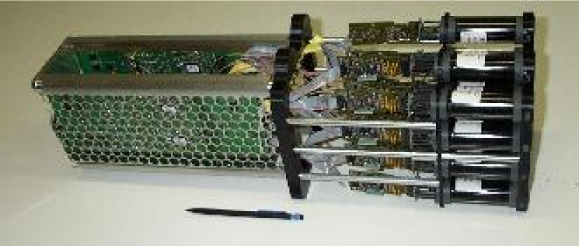
Figure 1: A camera drawer with its 16 PMTs, the individual HV supplies for each PMT, the two 8-channel acquisition cards and the control/interface card.

Figure 2: Schematic illustration of the electronics of one acquisition card ($8$ PMTs).

The high-gain channel is sensitive to single photoelectrons: the number of ADC counts between the pedestal and the signal from a single photoelectron is set to be $\approx 80$ ADC counts (for a PMT gain of $2\times 10^{5}$). This value is chosen such that the single photoelectron peak can be clearly distinguished at normal pixel operating high voltage (HV). The electronic noise of the system is such that the pedestal width is typically 20% of a photoelectron ($\approx 16$ ADC counts RMS). The low electronic noise and good sampling allow a precise gain calibration of every pixel.

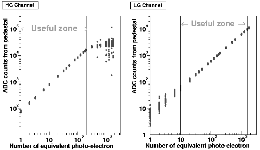
Figure 3: Linearity of the high gain channel (left-hand side) and low gain channel (right-hand side). Measured signal in ADC counts is shown against input signal in photoelectrons. The useful zones used for the analysis are shown.

2.2 PMT high voltage supply and slow control

In addition to the acquisition cards, a drawer contains a number of monitoring functions including three temperatures sensors, as well as individual high voltage supplies for each channel, which are controlled by the control/interface board. The high voltage supplies are DC-DC converters with active regulation for the cathode (on negative high voltage) and the four last dynodes. The high voltage is set via an analogue level supplied by the control board, and is adjusted to provide a uniform PMT gain across the camera. In order to minimise transit time differences between PMTs caused by the different high voltages applied, PMTs were sorted into drawers and cameras according to their gain. A high voltage divider and ADC allows the actual high voltage to be read back. In order to monitor pixel performance and to identify pixels receiving light from stars, both the total current provided by the high voltage supply to the PMT and the divider chain (“HVI”) as well as the DC anode current (“DCI”) are monitored. The “DCI” current depends on the PMT illumination and the electronic chain offset.

2.3 Calibration parameters

Standard Cherenkov analysis use as a starting point the signal amplitude of each pixel. The amplitude is the charge in p.e. induced by light on the PMT, this charge being corrected by the relative efficiency of this pixel compared to the mean value over the camera (“flat-fielding”, see Section 7). The calibration provides the required conversion coefficients from ADC counts to corrected photoelectrons.

For each event, ADC counts are measured in both channels, $ADC^{HG}$ for the high gain channel and $ADC^{LG}$ for the low gain channel. The calculation of the amplitude in photoelectrons received by every pixel is, for both channels:

$$\qquad\qquad A^{HG} = \frac{ADC^{HG}-P^{HG}}{\gamma_{e}^{ADC}}\times FF$$

$$\qquad\qquad A^{LG} = \frac{ADC^{LG}-P^{LG}}{\gamma_{e}^{ADC}}\times(HG/LG)\times FF$$ (1)

where,

• $P^{HG}$ and $P^{LG}$ are the ADC position of the base-line for both channels, which are the pedestal positions,

• $\gamma_{e}^{ADC}$ is the gain of the high gain channel in ADC counts per p.e.,

• $HG/LG$ is the amplification ratio of the high gain to the low gain,

• and $FF$ is the flat-field coefficient.

The flat-field coefficient corrects for different optical and quantum efficiencies between pixels within a camera.

For the image analysis, $A^{HG}$ and $A^{LG}$ are used to provide a single pixel amplitude. Provided that both gain channels function properly, the HG value alone is used up to $\approx 150$ p.e. (see Figure 3) and the LG value beyond $\approx 200$ p.e. For intermediate values, a weighted average of the HG and LG values is used and the amplitude is given by:

$$\qquad\qquad A=(1-\epsilon)\times ADC^{HG}+\epsilon\times ADC^{LG}$$ (2)

where $\epsilon\approx(ADC^{HG}-150)/(200-150)$.

To conclude, for both channels of every pixel, the calibration must provide the pedestal positions, the high gain $\gamma_{e}^{ADC}$, and the ratio of the high gain to the low gain. As the flat-fielding coefficients do not depend on the electronics, they are calculated per pixel and not per (HG or LG) channel as will be seen later (see Section 7). It is also essential that any non-operational channels or pixels are identified in the calibration process in order to avoid miscalculation of amplitudes.

3 Timing of the readout window

A time window containing only $N_{L}$ cells (from the 128 available) is read from the ARS (see Section 2.1). These cells are selected as follow. When the reading command is received, the ARS stops sampling and the first cell of the readout window is the $(128-N_{d})^{th}$ sample in the past from the latest filled sample in the circular buffer. $N_{d}$ is the time between the moment the signal is received by the pixel and the moment the trigger signal comes back to the drawer. The $N_{d}$ value has then to be calibrated in order that the Cherenkov signal integrated over the $N_{L}$ cells is maximised.

The position of the readout window (the $N_{d}$ value) is verified frequently using the sample mode facility of the ARSs. In this mode, the charge of the $N_{L}$ cells (each of 1 ns) is read and stored. The pulse shape can be then studied, as well as the readout timing. The position of the charge peak in the readout window is used to adjust the timing.

Figure 4 gives an example of data from a sample mode run made with air-shower events. The electronic noise in each cell, obtained using events which do not contain contributions due to Cherenkov light, is subtracted to extract the pulse shape. They are averaged over the HG channel for each telescope. From the ARS sample mode, the accuracy of timing of the readout window is about 1 ns.

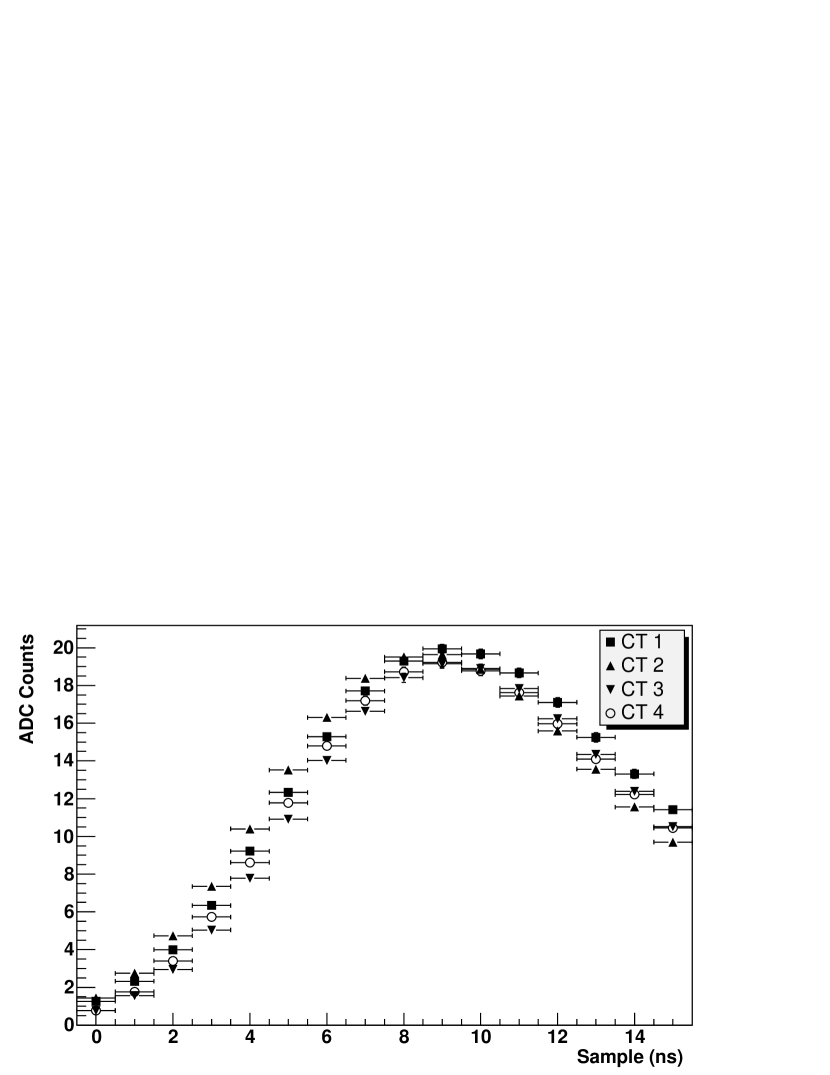
Figure 4: Mean signal samples over HG channels for the four cameras for air-shower events.

4 Estimation of pedestals

The pedestal position is defined as the mean ADC value recorded in the absence of any Cherenkov light.

In the dark, electronic noise creates a narrow Gaussian ADC distribution whose mean is the pedestal position. However, the pedestal position has some dependence on camera temperature, which varies between $20^{\circ}$C and $40^{\circ}$C depending on the season and the weather. The typical temperature variation during a run is of the order of $1^{\circ}$C. The pedestals must therefore be calculated for all channels during time-slices as short as possible to minimise the impact of pedestal drift due to temperature variations in the electronics.

During observations, the pixels are illuminated by night-sky background (NSB) photons, greatly increasing the pedestal width. There is over 1 p.e. of NSB per readout window in normal operation. Due to the capacitive coupling of the PMT signals to the ARS (see Figure 2) the pedestal position remains constant in the usual NSB range in Namibia. The mean pedestal position therefore corresponds to the position in ADC counts of zero photoelectrons of Cherenkov light.

4.1 Dark pedestal

To measure precisely the electronic noise in all channels, ADC distributions are taken in the absence of background light. The lids of all cameras are closed and the ADC distributions are randomly measured by software triggering of the cameras when the internal camera temperature is stable.

The resulting pedestal is determined by the base-line voltage of the electronic channels at the input of the ADC. These base-lines are approximately $-0.9$ V for both channels, corresponding to $\approx-730$ ADC counts. In charge mode, after the summation of the $16$ samples, the ADC counts are then $\approx-11500$ ADC counts: this is the typical electronic pedestal position. Measured pedestals lie in the range from -13000 to -11000 ADC counts. Random noise from PMTs and from electronic components is responsible for the pedestal width (see Figure 5). The noise at the input of the ADC is about $20\,\mathrm{mV}$ in the high-gain channel, which gives a pedestal RMS of $16$ ADC counts or about 0.2 p.e., and $7\,\mathrm{mV}$ in the low-gain channel, which gives a pedestal RMS of $6$ ADC counts or about 1 p.e.

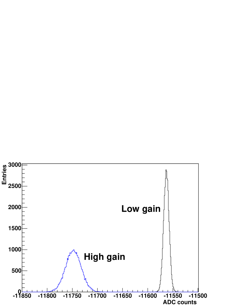
Figure 5: ADC distributions of dark pedestals for the high and low gain channels of a single pixel.

Runs taken with the camera lids closed can also be used to measure the drift of pedestal values with temperature using the temperature sensors mounted at three positions in every drawer. The dark pedestal position is correlated with temperature. The overall behaviour is a decreasing pedestal position for increasing temperature. As the shift can be as large as -50 ADC counts/degree, pedestal positions for observation runs must be calculated frequently (roughly every minute) to achieve the required precision ($\ll$1 p.e.).

4.2 Pedestal with night-sky background

During an observation run, the NSB modifies the ADC distributions of pedestals. As the coupling between PMT and ARS behaves like a RC circuit, the short photoelectron pulses (of positive polarity due to the inverting amplifiers) are followed by a slight negative undershoot over a few micro-seconds. For typical NSB rates, of order 100 MHz (in units of p.e. per second), the time between NSB photoelectrons is short compared to the time constant of the undershoot. The undershoots combine and average, causing a negative shift of the base-line, onto which NSB photoelectron signals are superimposed in a way that the overall average level remains at the dark-pedestal value.

When pedestals are measured during observation runs, the resulting distributions depend on the level of the NSB. For low NSB, it can happen that no NSB photoelectron arrives within the 16 ns integration window (see Section 2.1); in this case the measured pedestals have a similar narrow width to the dark pedestals, but exhibit a negative shift. Combining such events with events with one or more NSB photoelectrons which are fully or partly contained in the integration window, one finds a pedestal distribution with a sharp rise and peak at the location of the shifted dark pedestal, followed by a smeared single-photoelectron peak and a tail towards higher values (distribution for 50 MHz NSB in Figure 6).

At higher NSB levels, well above 100 MHz, there are usually several photoelectrons within the integration window and the pedestal distribution is essentially Gaussian, with a width given by the square root of the mean number of NSB photoelectrons (up to small corrections for the electronic noise, the width of the single-photoelectron amplitude distribution and the effect of photoelectron signals truncated by the integration window). The two other distributions shown in Figure 6 for 110 MHz and 140 MHz NSB rates represent intermediate cases, where the asymmetric shape of the Poisson distribution in the number of photoelectrons in the integration window is still visible.

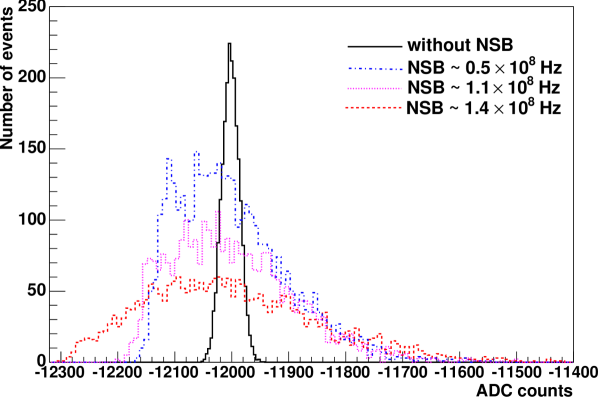
Figure 6: ADC distributions of pedestals at different night-sky background rates in real data.

Pedestals for observation runs are determined as often as possible in order to account for camera temperature variations. As a shower image contains typically only 20 pixels, real triggered events are used to measure pedestals. Pixels containing Cherenkov light are rejected. To identify such image pixels, amplitudes (in p.e.) are roughly calculated using the previously-calculated pedestal and using the nominal gain of channels (80 ADC counts per p.e. for the HG and 6 for the LG). For a given pixel, if neighbouring pixels have a signal amplitude above a threshold (around 1.5 to 3 p.e.) or if its own amplitude is above a threshold, this pixel is suspected to be contaminated by Cherenkov light. So this pixel’s value for this event does not contribute to this pixel pedestal histogram. This algorithm is applied for all pixels and all events until there are enough entries in pedestal histograms to determine accurately the pedestal positions from the mean of the histogram. The frequency of pedestal updates depends on the event rate of the observation run; pedestals are calculated approximately every minute.

5 Estimation of night-sky background

Knowledge of the actual NSB rate in each pixel – possibly influenced by a star in the field of view of the pixel – is important to judge if a pixel can be included in the image analysis. The NSB rate can be determined in two ways, from the pedestal width as illustrated in the previous section, and from the PMT currents.

5.1 NSB from pedestals width

One method to estimate the NSB brightness is to use the pixel pedestal widths. This technique is used as standard by the VERITAS collaboration [10]. During an observation, the pedestal width is dominated by NSB photon fluctuations. The typical pedestal RMS is about 100 ADC counts for the HG channel, corresponding to roughly 1.2 p.e. The NSB rate is estimated from the square of the pedestal width (subtracting the electronic noise and the charge dispersion of a single photoelectron in quadrature):

$$F_{NSB}=\sqrt{RMS_{P}^{2}-RMS_{0}^{2}-\sigma_{\gamma_{e}}^{2}}\,/\,(N_{L}\,\tau)\,\,\mathrm{Hz}$$ (3)

where $RMS_{P}$ is the pedestal RMS in p.e., $RMS_{0}$ is the electronic pedestal RMS in p.e., $\sigma_{\gamma_{e}}$ is the charge dispersion in p.e. of a single photoelectron and $N_{L}\times\tau\,=\,16\times 10^{-9}$ is the readout window in seconds. This expression should be accurate within 10-20% considering the corrections mentioned earlier.

5.2 NSB from PMTs currents

Because of its small temperature dependence and its larger range, the total current drawn by each PMT from the HV supply (HVI) is used to estimate the NSB, rather than the anode current (DCI). The HVI current is composed of the current drawn in the absence of illumination (mainly the divider current, proportional to the high voltage) and a component which increases linearly with the anode current. The shift of the HVI current from its dark value against DC p.e. flux ($F_{NSB}$) is shown in Figure 7. The relationship is described by Equation 4.

$$F_{NSB}=(3.235\pm 0.006)\times 10^{7}\times\Delta HVI_{\mu A}$$ (4)

To estimate the NSB with this method, one needs to know the values of the HVI in the dark. Values of the HVI base-lines, $\mathrm{HVI_{0}}$, are extracted regularly from runs taken with the camera lids closed. The ADC used to measure HVI has a very small temperature dependence (with slopes in the range -0.02 to +0.03 $\mathrm{\mu A/}$^∘C) compared to the current produced by normal values of NSB, $10^{2}$ MHz, which is of the order of 3.2$~{}\mathrm{\mu A}$. This temperature dependence can be neglected in the estimation of NSB.

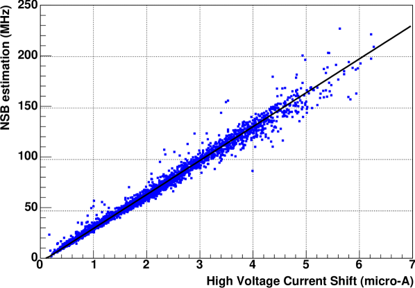
Figure 7: Offset-subtracted HVI current as a function of NSB brightness for all the pixels of one camera, measured in a test setup with controlled illumination.

The correlation between the two estimates of the NSB is given in Figure 8 for one camera for a single observation run, and are in reasonable agreement. A NSB rate of 250 MHz corresponds approximately to the presence of a star of magnitude $\sim 4$. Pixels with noise levels above this can be treated differently in the Cherenkov image analysis and are flagged as noisy.

Figure 8: Correlation of NSB estimates using HVI and pedestal width. The y-error bars are the RMS of the y-distribution. The line drawn corresponds to a perfect correlation.

6 Conversion factor between ADC counts and signal charge

The PMT signal, $V_{PM}$ (see Figure 2), is measured across a resistor and is amplified into two acquisition channels, one with low gain $G^{LG}$ and the other with high gain $G^{HG}$. The amplified signals are then converted into a digital signal with $\tau=1$ ns samples and summed over 16 ns. The conversion factor of the ADC is approximately $V_{ADC}$=1.22mV/Count. The number of (summed) ADC counts equivalent to one photoelectron is (for both readout channels $i$):

$$\qquad\qquad\qquad\gamma_{e,i}^{ADC}=\frac{G^{i}}{\tau\,V_{ADC}}\,\int V_{PM,s.p.e.}(t)~{}\mbox{d}t$$ (5)

Here $V_{PM,s.p.e.}$ is the single photoelectron pulse shape. We define the pixel gain as this conversion factor. This factor includes the PMT gain, the signal amplification in both readout channels and the integration in the ARS.

6.1 LED pulser for single-photoelectron illumination

Special runs are taken roughly every two days to determine the pixel gains. In these runs a LED pulser is used to illuminate the camera with an intensity of about 1 photoelectron/pixel. The LED and a diffuser are installed two meters in front of the cameras in their shelter. The light intensity homogeneity over the camera is $50$ %. The calibration LED is pulsed at 70 Hz and the same signal which pulses this LED is used to trigger the camera acquisition (after a suitable fixed delay) such that the signal arrives centered in the readout window (as explained in Section 3).

6.2 Determination of the gain of the HG channel

The pixel gain can be extracted from data taken under $\sim 1$ photoelectron illumination via a fit to the ADC count distribution of each pixel. The ADC distribution fit function is derived from the following assumptions: the number of photoelectrons follows a Poisson distribution, the electronic noise is much smaller than the width of the single p.e. distribution, and the 1 p.e. distribution is described by a Gaussian distribution. Then, the electronic pedestal is approximated by a Gaussian with a standard deviation $\sigma_{P}$ and with a mean position in ADC counts $P$. The light distribution for a given signal of $n$ p.e. ($n\in\mathbb{N}$) is approximated also by a Gaussian with a standard deviation $\sqrt{n}~{}\sigma_{\gamma_{e}}$ and with a mean position in ADC counts $P+n\,\gamma_{e}^{ADC}$, $\gamma_{e}^{ADC}$ being the conversion factor between ADC counts and photoelectrons and $\sigma_{\gamma_{e}}$ is the RMS of the charge induced by a single photoelectron. Under a mean light intensity $\mu$ the expected signal distribution is given by:

$$\mathcal{G}(x)=N\times \bigg{(} \frac{e^{-\mu}}{\sqrt{2\pi}\sigma_{P}}\,exp\bigg{[}-\frac{1}{2}\Big{(}\frac{x-P}{\sigma_{P}}\Big{)}^{2}\bigg{]}$$ (6)

$$+ \kappa\sum_{n=1}^{m\gg 1}\frac{e^{-\mu}}{\sqrt{2\pi}\,\sigma_{\gamma_{e}}}\frac{\mu^{n}}{n!}\,exp\bigg{[}-\frac{1}{2}\Big{(}\frac{x-(P+n\,\gamma_{e}^{ADC})}{\sqrt{n}\,\sigma_{\gamma_{e}}}\Big{)}^{2}\bigg{]}\bigg{)}$$

This function is used to fit the signal distribution of each pixel. All parameters are free except the overall normalisation $N$ which is fixed according to the number of events in the run. The normalisation $\kappa$ should be equal to one for a Poissonian statistics and can also be adjusted. A sample signal distribution and fit are shown in Figure 9.

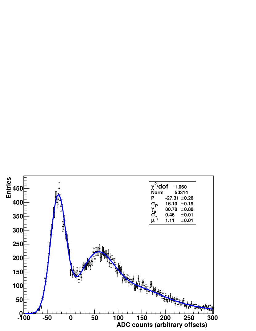
Figure 9: Example of an ADC count distribution for a single-photoelectron run.

The high-gain values of $\gamma_{e}^{ADC}$ for the four telescopes are given in Table 1. In January 2004 the mean gains are close to the nominal value of 80 ADC counts per p.e. and their RMS is around 2-3 ADC counts for all telescopes. The distributions of $\gamma_{e}^{ADC}$ over pixels are almost Gaussian and the pixel gains are randomly distributed within the cameras.

Telescope	$\gamma_{e}^{ADC}$		$HG/LG$		$FF$
	mean	RMS	mean	RMS	RMS
CT 1	79.8	1.8	12.98	0.44	0.10
CT 2	79.4	3.0	13.73	0.43	0.11
CT 3	76.8	3.5	13.32	0.47	0.13
CT 4	77.3	3.8	13.52	0.63	0.09

Table 1: Summary of mean values of calibration coefficients in January 2004, and of their variation across pixels in a camera. The high-gain $\gamma_{e}^{ADC}$ values are given in ADC counts. By definition, the mean flat-field coefficient is 1.

However, the fit may fail when the light intensity $\mu$ of the $\gamma_{e}^{ADC}$ measurement is too low or too high or when the corresponding ARS does not work properly (see Section 9). No gain estimate is then available for this pixel and a gain of 80 ADC counts/p.e. is assumed. In this case, the flat-field coefficient compensates for any deviation from the nominal gain (see Section 7).

Laboratory measurements show that the single photoelectron distribution of the Photonis XP2960 PMTs used by H.E.S.S. is significantly non-Gaussian. The fit to the signal distribution assuming a Gaussian shape leads to a bias of a few percent in the determined gain. This bias is included and accounted in our simulations (which use the measured single-p.e. distribution).

6.3 Determination of the gain of the LG channel

In the regime where both gain channels are linear (30 to 150 p.e. in order to be conservative - see Figure 3) the ratio of the signals provides a measurement of the amplification ratio in the two channels. With the previously calculated gain for the HG channel and with this amplification ratio, the gain of the LG channel can be calculated.

Cherenkov events from normal observations are used to measure these gain ratios. Using nominal gains, approximate pixel charges are determined and pixels with charges in the overlap regime are selected. The mean ratio of the pedestal-subtracted ADC counts in both channels for these selected events is used to estimate the amplification ratio for each pixel.

The gain ratios for all cameras are given in Table 1. The mean ratios are around $13.5$ (with RMS $\sim 0.5$). The slight differences are due to the gain dispersion of the amplifiers.

7 Flat-field coefficients

Different photocathode efficiencies and different Winston cone light collection efficiencies [2] produce some inhomogeneity in the camera. Thus, even after the calibration of the electronic chain, channels exhibit a slightly different response to a uniform illumination. Flat-field coefficients (FF) are used to correct for these differences.

The flat-field coefficients are determined from special flat-field runs (taken roughly every 2 days) which use LED flashers [11] mounted on the telescope dishes at 15 m from the cameras to provide uniform illumination. The flashers produce short pulses (FWHM of 5 ns) with uniform illumination out to 10^∘ (bigger than the angular size of the camera). The wavelength range of these pulses is 390 to 420 nm, around the wavelength of PMT peak quantum efficiency. The pulse intensity is stable within 5% RMS and can be adjusted by the use of 5 different neutral density filters, giving an operating range of 10 to 200 p.e. The camera is triggered in the same way as for Cherenkov showers but with an increased pixel multiplicity ($>$9 pixels) to reduce the background of air-showers.

Flat-field coefficients are extracted from flat-field run data using calibrated amplitudes without the FF correction. For each event the mean signal over each camera is calculated, excluding unusable pixels (determined as described in the Section 9). The ratio of each pixel signal to this mean signal is accumulated in a histogram. The mean of this ratio over the run gives the efficiency of each pixel relative to the camera mean. The inverse of this mean value, the flat-field coefficient (FF), is used to correct for pixel efficiency differences. By definition, the mean FF is equal to 1. The distribution of flat-field coefficients gives an estimate of the uniformity of each camera. As can be seen from Table 1, the typical RMS of the FF distribution is $\approx 10$%.

8 Stability of calibration parameters

8.1 Stability within a lunar cycle

It is expected that the calibration coefficients are stable over periods of weeks if the PMT high voltage is not changed. During each observation period (corresponding to a lunar cycle) several measurements of each calibration value are made for every pixel. The RMS variation of these measurements is used to characterise the stability of the calibration parameters. The values of the RMS variation of parameters, averaged over all channels of a camera, are summarised in Table 2 for the January 2004 period (during which no HV adjustments were made). As expected, all calibration parameters were stable at the few percent level during this period for all cameras.

Telescope	CT 1	CT 2	CT 3	CT 4
$\gamma_{e}^{ADC}$: average RMS variation	2.1%	3.4%	3.6%	3.4%
$HG/LG$: average RMS variation	1.4%	1.2%	1.2%	1.2%
$FF$: average RMS variation	0.8%	0.9%	0.8%	1.0%

Table 2: Summary of the stability of calibration parameters in the January moon cycle of 2004. Shown is the RMS variation in time of the different parameters; the RMS values are averaged over all channels of a camera.

The majority of calibration coefficients are affected by changes to the PMT HV. The PMT gains are proportional to $V^{\alpha}$, with $\alpha\approx 5.2$. The flat-field coefficients are also a function of HV via the collection efficiency of PMTs (collection efficiency of electrons between the photo-cathode and the first dynode). Only the gain ratio of the two electronics channels is independent of HV. A complete re-calibration is therefore required when HV adjustments are made (roughly every 3-6 months).

8.2 Merging of calibration parameters

Given the stability of calibration parameters on the time-scale of weeks it is reasonable to merge values taken during stable periods to improve the accuracy of the calibration parameters. The reasons for this merging are as follows. In a single calibration run there are typically a few pixels which are not well measured due to one of the problems described in Section 9. The merging also reduces the statistical error on the final coefficients measurements, and ensures that remaining systematic effects such as temperature dependencies are much reduced.

The first step of the merging process is to identify periods with constant HV settings during at most one lunar cycle. If the PMT HV has been adjusted during a lunar cycle (to compensate for the decreased gain caused by PMT aging), two calibration periods are created around the HV change. A summary of the merged parameter values within each camera is given in Table 1 for the January 2004 calibration period.

Several precautions are taken to ensure the reliability of the merged values. Pixels which experience problems within calibration runs are identified using the techniques described in Section 9. In addition calibration runs with a temperature drift of more than 0.5^∘ C are excluded from the merging to guard against biases introduced by ADC pedestal drifts.

8.3 Long term variations of calibration parameters

On time-scales longer than one month, the effects of PMT aging and possibly mirror degradation may become apparent. Figure 10 shows the evolution of PMT gain over 1 year. The mean gain of each camera is shown for each dark moon period. The general trend is for gains to decrease with time until a HV adjustment is made. The high voltages were increased for CT2 in October and December 2003, for CT4 in November and for CT3 in December.

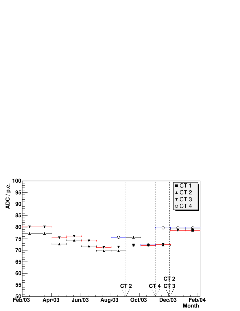
Figure 10: Evolution of the mean $\gamma_{e}^{ADC}$ per camera in 2003/04. The large arrows correspond to an HV increase for the labelled telescope. Telescopes were installed in the following order: CT3, CT2, CT4 and CT1.

The HG/LG ratios do not depend on PMT HV and are expected to be stable. The time evolution of the mean ratio in each camera is given in Figure 11.

After December 2003, all drawers were swapped between cameras to further improve the HV homogeneity within each camera. As a consequence, the HG channel gains and gain ratios of January 2004 are not directly comparable with earlier periods.

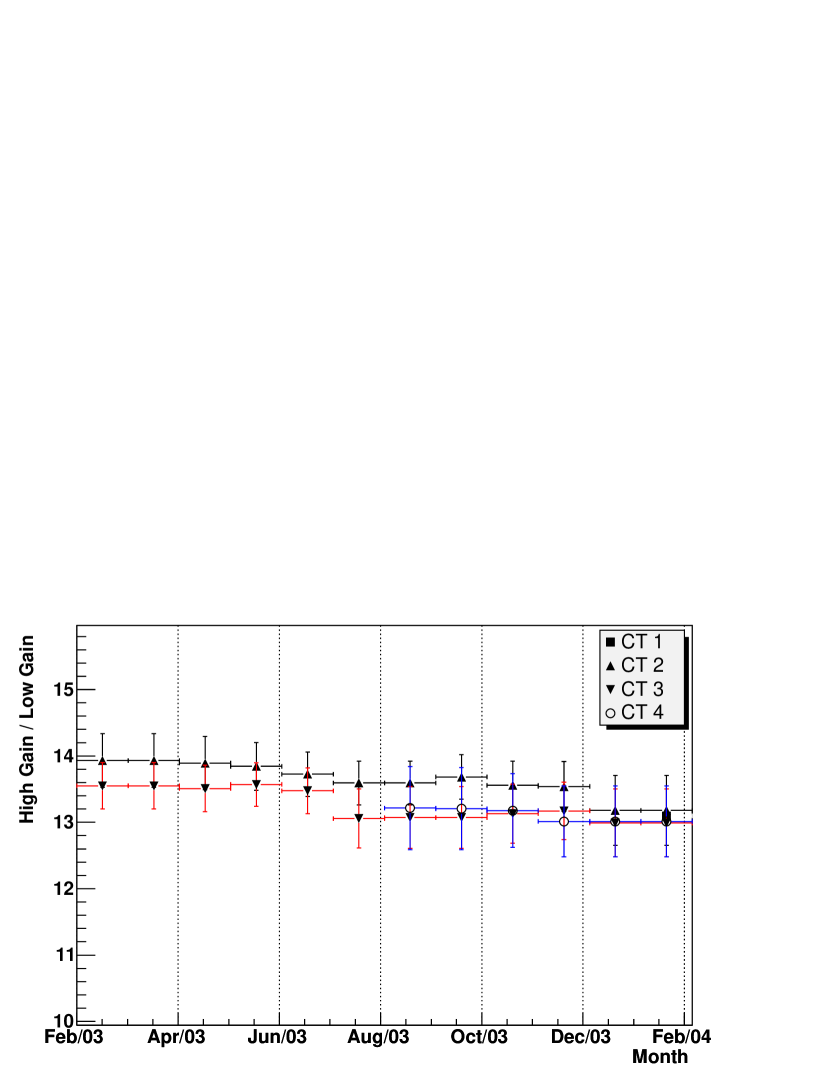
Figure 11: Evolution of the mean HG/LG ratio per camera in 2003/04.

9 Identification of unusable channels

In any given run, there are typically a few pixels with characteristics that make them unsuitable for use in Cherenkov image analysis. In such cases it may be possible to use the other gain channel to calculate the signal amplitude (depending on its value).

9.1 Missing calibration coefficients

As described in section 8, pixel calibration coefficients are merged (averaged) for periods in which the pixel gains are considered stable. Even after this merging process a small number of pixels do not have useful calibration coefficients. The most common reason for this is that the pixel is broken or seriously damaged at the hardware level. The affected gain channels of such pixels are excluded from the analysis.

9.2 Failure to synchronise the analogue memory

When an ARS works properly, the signals of the four associated channels are centred in the readout window of 16 ns. The integrated signal of such channels is at maximum. When an ARS is unlocked, the readout window is misplaced because of timing problems in the window positioning and the integrated signal is low and unpredictable. As a consequence, the four channels served by this ARS are not usable.

This problem appears randomly on the ARSs every time the power is switched on. For a given camera and gain channel the number of unlocked ARSs ranges from 1-5. Since the high-gain and low-gain channels of a pixel are read out by different ARSs (see Figure 2), it is, however, rare for both the HG and LG channels of a single pixel to be unlocked. An estimate of signal amplitude is therefore usually still available for these channels.

The distribution of the charge ratio between channels used in the determination of the amplification ratio is also used to identify unlocked ARSs. If one of the gain channels of a pixel is unlocked, the mean signal of the corresponding channel is less than expected and the signal ratio distribution is modified. The RMS of the signal ratio is increased and the mean value differs from the merged gain ratio of this period (see Section 10). The RMS and the distribution shape are used to flag the probably unlocked channels. An ARS is flagged as unlocked if at least two pixels from four have such amplitude ratio behaviour. Sample amplitude-ratio histograms are presented in Figure 12 for pixels with locked and unlocked ARSs.

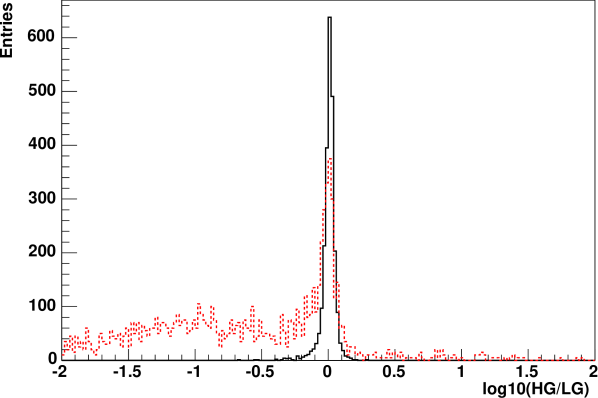
Figure 12: Example of pixels on CT2 with a locked (continuous line, RMS=0.06) and an unlocked ARS in the high gain channel (dashed line, RMS=1.0). The distribution is the logarithm of the ratio of the charges calculated from the high and low gain channels in the range 15-150 p.e. The nominal value of this parameter is 0.

9.3 Other pixel problems

The pixel high voltage monitoring information is taken at a rate of $\sim 2$ Hz. Pixels with any deviation during a run of greater than 10 V are excluded from the analysis.

Pixels with a very low frequency of large signals ($>30$ p.e.) are also excluded. Such pixels may have a broken PMT base or a damaged photo-cathode. Pixels with a very high frequency of signals above the same threshold are also excluded, bit errors in the digital cards of drawers are suspected in this case.

In addition to pixels with hardware problems there are typically a few pixels in every field-of-view that are affected by bright stars. One of the techniques described in Section 5 is used to identify these pixels.

These additional hardware problems occur at the $<1$% level.

9.4 Summary of channel problems

Table 3 summarises the mean number of channels that are considered unusable out of the 1920 electronics channels of each camera in January 2004. This table illustrates that only a small fraction of pixels are unusable during observations: less than 2% of the LG and HG channels have an unlocked ARS and less than 0.1% of the channels have other hardware problems. The lack of calibration coefficients affects less than 2% of the channels. The fraction of unused channels per run is then of the order of 3% to 4%. The mean fraction of images where a pixel is completely missing due to hardware problems is 1-2%.

Telescope	CT 1	CT 2	CT 3	CT 4
Lack of coefficients	11	13	23	22
Unlocked HG ARS	6.2	10.6	8.2	13.5
Unlocked LG ARS	15.6	13.1	13.6	18.0
Hardware problem	0.4	0.9	2.3	0.4
Noisy pixels (Electronics)	4.4	0.8	1.1	3.0

Table 3: Summary of identified pixels problem. These number are the average number of channels with problems (HG or LG) in January 2004. There are 1920 channels in total in each camera.

9.5 Choice of the channel

The pixel amplitude used in the analysis may be based on the high gain ADC value or the low gain value or a combination of both, as discussed in Section 2.3. The choice of the channel to be used for a pixel depends on the amplitude of each channel and the existence of any identified problems with one of the gain channels. Normally, the HG channel is always preferred for intensities below 150 p.e. and the LG channel above 200 p.e. However, in the case of an unusable HG channel the LG channel is used down to 15 p.e. In the case of an unusable LG channel, the HG channel is used up to 200 p.e.

If a pixel has no usable channel, or has a signal amplitude outside of the linear range of its only available channel, its signal is set to 0 p.e. As mentioned in Section 6.2, if no high gain ($\gamma_{e}^{ADC}$) is avaible, flat-fielding coefficient compensate for any deviation from the nominal gain and then the pixel is usable. But, if no high gain ($\gamma_{e}^{ADC}$) and no flat-fielding coefficient are available, the pixel is completely excluded. If no gain ratio is available, only the high gain channel is used.

10 Accuracy of calibration parameters

10.1 Pedestal position

As described in Section 4, the ADC pedestal positions depend on temperature. They must therefore be calculated as frequently as possible to avoid base-line drifts. To verify that the calculation frequency is high enough, a method has been developed to measure the accuracy of the pedestal positions.

A typical Cherenkov image involves only $\sim$20 camera pixels. The remaining 98% of the camera measures only NSB around the pedestal position. Pixels which are not found in a cluster after tail cuts (see [12, 10] for a description of tail cuts technique), are considered to be unaffected by Cherenkov light. The mean amplitude of pixels selected in this way gives an estimate of the pedestal position. The precision of the pedestal position can be estimated by comparing this value with the previously estimated position.

This method has been applied to an observation run with a large temperature variation (amplitude of the order of 1^∘C). The average residual amplitude over the camera is calculated for each new pedestal. This average is constant in time and is around 0.05 p.e. The residual RMS across the camera is around 0.03 p.e. We can conclude that measurements of the high gain pedestal position are frequent enough and are accurate at the level of 0.05 p.e.

Two independent methods have been developed to compute the pedestal positions and calibration parameters. Concerning the pedestal evaluation, the differences consist mainly of different techniques for rejection of Cherenkov events. A comparison of these two methods provides a second estimate of the pedestal position accuracy. Table 4 gives the means and RMS of the differences of the pedestal positions for both channels of each pixel during one run in January 2004. The differences are given in photoelectrons. The two methods agree within 0.1 p.e. in the high gain channel and 0.5 p.e. in the low gain channel.

Telescope	CT 1	CT 2	CT 3	CT 4
HG: mean	-0.02	-0.03	-0.01	-0.01
RMS	0.08	0.03	0.06	0.13
LG: mean	-0.03	-0.15	-0.02	-0.06
RMS	0.38	0.17	0.49	0.36

Table 4: Summary of the differences between two methods to estimate channel pedestal. Shown are the mean and RMS of the difference over all channels of a camera, in units of photoelectrons.

10.2 Comparison of merged coefficients between independent calibrations

As was done for the pedestals, two independent approaches have been developed to derive the other calibration coefficients. The implementation details of the two calibration schemes differ, but the methods described in this paper are used in both. The differences are the adjustment or not of the normalisation parameter for the determination of $\gamma_{e}^{ADC}$ and a different event selection based on their amplitudes for the determination of $FF$ and $HG/LG$ coefficients. Table 5 gives the mean and RMS of the differences pixel to pixel of the calibration coefficients for a period in January 2004. The results are given as a percentage and show good agreement between the different schemes.

The most crucial calibration factor is the conversion factor from pedestal-subtracted high gain ADC counts to effective photoelectrons: $\gamma_{e}^{ADC}/FF$. The RMS differences between the independent schemes for this quantity are $<4$%. For the ratio of the two gain channels $HG/LG$ the different schemes agree at a similar level.

Telescope	CT 1	CT 2	CT 3	CT 4
$\gamma_{e}^{ADC}$: mean	1.1%	-2.0%	-0.5%	-1.8%
RMS	2.7%	3.0%	2.5%	2.8%
Flat-field: mean	0.3%	0.4%	-0.2%	0.0%
RMS	3.0%	4.0%	5.4%	2.9%
$\gamma_{e}^{ADC}/FF$: mean	0.8%	-2.4%	-0.8%	-1.9%
RMS	2.4%	1.1%	3.2%	1.1%
$HG/LG$: mean	0.1%	-1.9%	-1.5%	-2.2%
RMS	2.0%	0.8%	2.6%	1.2%

Table 5: Summary of the differences between two calibration schemes, for the calibration coefficients of every pixel. Shown are the mean and RMS of the difference distribution over pixels in a camera, given in percentage.

10.3 Verification of the flat-field coefficient calculation

To check the calculation and merging of flat-field coefficients, these coefficients are recalculated after application of the merged coefficients to the charge calculation. The newly calculated coefficients should be close to 1.0 and provide an estimate of the coefficient uncertainty.

For an example run taken in January the recalculated flat-field coefficients distributions are Gaussian and their RMS are $(0.006,0.006,0.01,0.008)$, respectively, for CT1, CT2, CT3 and CT4, implying an accuracy of $<1$%.

A completely independent estimate of flat-field coefficients can be made using muon ring images. As the Cherenkov emission of single muons is very well understood, it is possible to accurately predict the charge distribution and shape of the muon rings observed. For each muon ring, the particular geometrical parameters (impact distance, arrival angle, …) are fit to the image. The ratio of the actual and expected charges gives an estimate of the efficiency of every pixel on the ring. This method is described in detail in [13] and produces $FF$ coefficients that agree with the standard calculation at the few percent level. This level of agreement is encouraging given the completely different systematic errors associated with this independent method.

10.4 Comparison of unusable channels

Comparisons of unusable channels have also been made between the two calibration techniques. Except for one or two channels per camera, the identified unlocked ARSs are identical. Concerning the other types of problems, the agreement is generally good, in spite of different methods for unusable channel identification.

11 Summary

Elaborate calibration procedures have been developed and implemented for the four cameras of the H.E.S.S. detector. The calibration algorithms and the monitoring of calibration coefficients monitoring are automated and their results are used in the standard data analysis. Two independent calibration schemes are available and are in good agreement. The flat-field coefficients have been evaluated by a different method using muon rings [13] and they are in agreement with the standard coefficients. In conclusion, the calibration of cameras appears to be robust and accurate.

Pixel amplitudes in units of effective (flat-fielded) photoelectrons should be accurate, for the usual amplitudes, within a pedestal error of less than 0.1 p.e. and a linear error of less than 5%, including systematic uncertainties introduced by the required assumptions about the exact shape of the amplitude distributions of single photoelectrons, relevant for the gain calibration. The statistical uncertainties are negligible compared to the systematic ones because of the high number of calibration runs and the high number of events.

The camera calibration does not provide the final absolute calibration of the H.E.S.S. detector, which includes the reflectivity of the mirrors and Winston cones and the absolute quantum efficiency of the PMTs. The absolute calibration can either be based on laboratory measurements of these quantities or on the use of muon rings; the latter approach will be presented in a separate paper. Moreover, the behaviour of the camera trigger has to be understood correctly in order to estimate the gamma ray detection rates. This is achieved using detailed simulations of air showers in atmosphere and of the detector, which will be described elsewhere in detail. The overall quality of the current understanding of the full calibration of the H.E.S.S. instrument is illustrated in Figure 13, where the flux determined for the Crab Nebula is compared with earlier measurements and where excellent agreement is found.

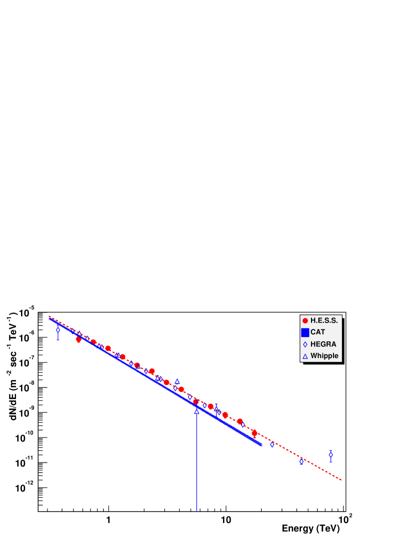
Figure 13: Spectrum of gamma rays from the Crab Nebula, reconstructed on the basis of the calibration techniques described in this paper, together with results from CAT [14], HEGRA [15] and Whipple [16]. The dashed line is the fitted spectrum of the H.E.S.S. data. See [17] for details.

References

- [1] Hofmann, W., Proc. 28th ICRC, Tsukuba (2003), Univ. Academy Press, Tokyo, p. 2811-2814
- [2] Bernlöhr, K., et al., Astropart. Phys. 20, 111-128 (2003)
- [3] Cornils, R., et al., Astropart. Phys. 20, 129-143 (2003)
- [4] Vincent, P., et al., Proc. 28th ICRC, Tsukuba (2003), Univ. Academy Press, Tokyo, p. 2887-2890
- [5] Barrau, A., et al., NIM A416, 278-292 (1998)
- [6] Armstrong, P., et al., Exp. Astronomy 9, 51-80 (1998)
- [7] Daum, A., et al., Astropart. Phys. 8, 1-11 (1997)
- [8] Pühlhofer, G., et al., Astropart. Phys. 20, 267-291 (2003)
- [9] Haller, G.M., Wooley, B.A., SLAC-PUB-6402 (1993)
- [10] Bond, I.H., Hillas, A. M., Bradbury, S. M., Astropart. Phys. 20, 311-321 (2003)
- [11] Noutsos, A., et al., Proc. 28th ICRC, Tsukuba (2003), Univ. Academy Press, Tokyo, p. 2975-2978
- [12] Reynolds, P.T. , et al., ApJ 404, 206-218 (1993)
- [13] Leroy, N., et al., Proc. 28th ICRC, Tsukuba (2003), Univ. Academy Press, Tokyo, p. 2895-2898
- [14] Masterson, C., et al., Proc. High Energy Gamma-Ray Astronomy 2000, AIP 558, 753-756 (2001)
- [15] Horns, D., et al., Proc. 28th ICRC, Tsukuba (2003), Univ. Academy Press, Tokyo, p. 2373-2376
- [16] Mohanty, G., et al., Astropart. Phys. 9, 15-43 (1998)
- [17] Aharonian, F.A., et al., to be published