Electron Temperatures in W51 Complex from High Resolution, Low Frequency Radio Observations

Abstract

W51 is a giant radio complex lying along the tangent to the Sagitarius arm at a distance of about 7kpc from Sun, with an extension of about 1^∘ in the sky. It is divided into three components A,B,C where W51A and W51B consist of many compact HII regions while W51C is a supernova remnant. We have made continuum radio observations of these HII regions of the W51 complex at 240,610,1060,1400 MHz using GMRT with lower resolution ($20^{\prime\prime}$ $\times$ $15^{\prime\prime}$) at the lowest frequency. The observed spectra of the prominent thermal subcomponents of W51 have been fitted to a free-free emission spectrum and their physical properties like electron temperatures and emission measures have been estimated. The electron temperatures from continuum spectra are found to be lower than the temperatures reported from radio recombination line (RRL) studies of these HII regions indicating the need for a filling factor even at this resolution. Also, the observed brightness at 240MHz is found to be higher than expected from the best fits suggesting the need for a multicomponent model for the region.

Keywords: ISM,HII regions,radio continuum,individual(W51)

1 Introduction

W51 is a giant radio emitting complex, lying along the tangent to the Sagitarius arm at a distance of about 7kpc and having an angular size of about 1^∘. The complex consists of many HII regions of varying morphologies and compactness, embedded in an extended and diffuse emission. According to convention adopted by Kundu & Velusamy(1967) the source is divided into 3 components, W51 A and B being a collection of compact HII regions while W51C is a nonthermal source that is identified with a supernova remnant (Copetti & Schmidt 1991). The entire complex is optically obscured but has been extensively observed at radio frequencies and the early observations have been reviewed by Bieging(1975). The brightest HII regions are found in W51A, which itself consists of two subcomponents G49.5-0.4 and G49.4-0.3.  G49.5-0.4 is the most luminous star forming region in the entire complex and has been studied in detail. High resolution radio continuum observations (Martin 1972; Mehringer 1994; Subrahmanyan & Goss 1995) have identified atleast 8 prominent compact sources in G49.5-0.4 which are referred to as G49.5-0.4 a,b,…,h in order of increasing right ascension. Similarly, G49.4-0.3 consists of atleast 3 compact sources G49.4-0.3 a,b,c (Martin 1972).

Radio recombination line (RRL) studies of G49.5-0.4 have been used to study the kinematics and local thermodynamic equilibrium(LTE) electron temperature($T_{e}$) of this region. H109$\alpha$ RRL observations by Wilson et al(1970) with a resolution of $4^{\prime}$ and by Pankonin et al (1979) with a resolution of $2.6^{\prime}$ show that $T_{e}\sim$6000K in G49.5-0.4. Lower frequency observations for H137$\beta$ and H166$\alpha$ lines show higher temperatures of 8500K and 7100K respectively (Pankonin et al 1979). Since lower frequency lines are expected to arise from outer low density parts of the HII regions, this results suggest that there is a temperature gradient that increases radially outwards (Churchwell et al 1978). From observations of H92$\alpha$ lines Mehringer(1994) concludes that $T_{e}$ varies from 4700 to 11000K for the different components with an average of 7800 $\pm$ 1200K. All the RRL results quoted above have been derived under the LTE approximation.

The electron temperature is one of the most important parameters in understanding the physical properties of thermal HII regions. Low frequency continuum observations in the optically thick regime offer a direct estimate of the electron temperatures. Meter-wavelength observations at 410MHz by Shaver(1969) and at 151MHz by Copetti & Schmidt(1991) show that $T_{e}$ in G49.5-0.4 is 3500$\pm$700K and 4650$\pm$500K respectively. Since low frequency continuum observations also arise from the outer parts of HII region, these low temperatures suggest a radial decrease in temperature from the core, which is opposite to the trend seen in RRL studies. However, Subrahmanyan & Goss(1995), from 330MHz continuum observation with $\sim$$1^{\prime}$ resolution, infer a value of at least 7500K towards G49.5-0.4e, the brightest source in G49.5-0.4. It is possible that the low temperatures obtained by Shaver(1969) and Copetti & Schmidt(1991) is due to the poor resolution ($>3^{\prime}$) of their images.

In order to resolve this discrepancy and make an improved determination of the electron temperatures and other physical parameters in the component W51A, we have made high resolution continuum images of the HII regions in W51A using Giant Meterwave Radio Telescope (GMRT) at 240,610,1060, and 1400MHz. This is the first time that W51 has been observed at meter-wavelengths with arcsec resolutions.

Table 1: Observational Parameters

Central	Date	Bandwidth	Best	Primary
Frequency(MHz)		(MHz)	Resolution	Beam
240	9Mar2001	6.25	$19^{\prime\prime}\times 14^{\prime\prime}$ @50 ∘	$114^{\prime}$
616	30Aug2001	12.625	$6^{\prime\prime}\times 6^{\prime\prime}$	$43^{\prime}$
1057	5Jun2001	12.625	$3.7^{\prime\prime}\times 3.2^{\prime\prime}$ @82∘	$32^{\prime}$
1407	4Jun2001	13.25	$3^{\prime\prime}\times 3.5^{\prime\prime}$ @ -79∘	$24^{\prime}$

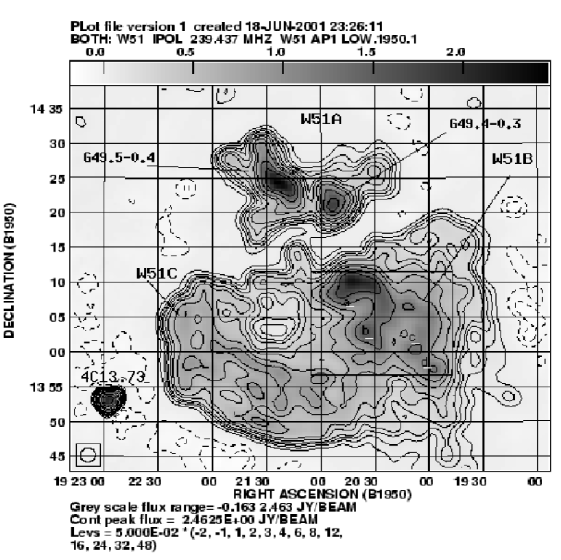
Figure 1: Map of full W51 complex at 240MHz with resolution of $2^{\prime}$. The rms noise is 21mJy.

2 GMRT Observations

2.1 Observations and Data Reduction

Full synthesis observations of the W51 complex were made with the GMRT during the year 2001. Details of the observational parameters are given in Table 1. All the observations were centred on W51A. While at the higher frequency the fields of view were restricted to only W51A, the 240MHz data had a field of view large enough to cover the entire W51 complex. The observations were made in the standard spectral line mode of GMRT (128 channels, each of 128KHz width) for nearly 8 hours at each frequency. A band pass calibrator, which was also the flux density calibrator (either 3C48 or 3C286 or both), was observed for 15-20 minutes at the beginning or at the end of the observation. The rest of the observation was devoted to W51, with a secondary calibrator observed every half an hour or so.

In the offline analysis, which was done using standard AIPS, the data were edited, the antenna bandpass estimated and the spectral channels collapsed to a continuum channel. For the 240MHz data, where bandwidth smearing is an issue, the spectral data was averaged to 5 channels of 1.25MHz each. The channel averaged data were calibrated using the secondary calibrator. At all observing frequencies, uniformly weighted maps were made with the full resolution of the GMRT, cleaned, and self-calibrated (two rounds of phase and one of amplitude) to make the final map. For images at 240MHz, wide field corrections were incorporated using the multiple facet imaging option in IMAGR. Since the resolution of GMRT varies with frequency, in order to compare the maps at the different frequencies, additional maps were made at the higher frequencies with lower resolution ($20^{\prime\prime}$ $\times$ $15^{\prime\prime}$) comparable with the resolution of the GMRT at 240MHz and the 5 and 1.4GHz maps presented by Mehringer(1994). It must be noted that the u-v coverages are different in the different maps which could lead to uncertainties in comparing the maps at different frequencies. A low resolution map $2^{\prime}$ of the full W51 complex was also made at 240MHz to compare with the existing images.

During the period of these observations, real time measurement of the system temperature was not available at the GMRT. The change in the system temperature between the primary calibrator and W51 was measured later and the flux densities in the final maps were corrected for this (correction factor ranged from 1.2 to 1.6). All the images were corrected for the primary beam of the GMRT antennas.

2.2 240MHz Image of the W51 Complex

Figure 1 shows full field map of W51 at 240MHz made with a resolution of $2^{\prime}$ . The overall features agree very well with the VLA map at 330MHz with similar resolution (Subrahmanyan & Goss 1995). The thermal sources W51A in the north and W51B in the centre, and the nonthermal source W51C are marked in the figure. The extended nonthermal emission from the supernova remnant W51C is clearly seen. The overall angular extent of the source is about $45^{\prime}$ and since the shortest spacing in our observations is 50 wavelengths at 240MHz, we believe that our 240MHz images are not seriously affected by the absence of measurements at short spacings. We have tried to alleviate this effect by using the ‘zero spacing’flux option in IMAGR and have carefully compared our integrated flux densities of the various components with those estimated by others ( Copetti & Schmidt 1991, Subrahmanyan & Goss 1995) to convince ourselves that our flux density estimates are correct. Inspite of this there is some evidence in Figure 1 for a negative bowl around the complex at about 50 mJy/beam and this has been included in the error estimate. While this could cause us to underestimate the flux density in the extended emission, its effect on the high resolution maps is negligible since the beam areas are smaller. Due to various systematic uncertainities, including the correction for $T_{sys}$, we believe that our flux density estimates are accurate to about $10\%$. This was further verified using the source 4C13.73 at the south-east boundary of W51. The source which is resolved into a double in the high resolution 240MHz images, has a flux density of 4.2$\pm$0.4 Jy at 240MHz which agrees within errors with estimates based on previous measurements at 151 and 330MHz (Copetti & Schmidt 1991, Subrahmanyan(private communication)).

The flux density observed for the W51 complex at 240MHz (Figure 1) is 305$\pm$ 30 Jy, out of which 46$\pm$ 4Jy lies in W51A. The integrated flux densities in the two subcomponents of W51A, G49.5-0.4 and G49.4-0.3, are 29$\pm$3 and 17$\pm$2Jy respectively. These flux densities are consistent with 330MHz measurements of Subrahmanyan & Goss (1995) with the proviso that these are thermal sources that become optically thick below 1GHz. The separation of the rest of W51 into W51B and W51C is slightly subjective and if done the way as shown in Figure 1, the total flux densities in W51B and W51C are 110$\pm$15 and 150$\pm$ 20 Jy respectively. The regions (marked a,b,c,d) in W51B corresponding to the sources G49.2-0.4, G49.1-0.4 and G48.9-0.3 (c,d) respectively, along with the connecting bridge of emission seen at higher frequencies (Subrahmanyan & Goss 1995, Altenhoff et al 1978), are visible in our map too, though all the condensations are fainter than in the 330MHz map of Subrahmanyan & Goss, confirming that they are thermal sources.

Our estimate of the integrated flux density of W51C is higher than that of Subrahmanyan & Goss(1995) but this could be due to different regions being included in W51C. A more useful quantity is the average surface brightness over W51C at 240MHz which, in the units used by Subrahmanyan & Goss (1995), we estimate to be 0.22 Jy/beam of $1^{\prime}$ FWHM, if we include the entire extent of the source including the fainter extensions to the south west. If we exclude this region, since this may be more appropriate for comparing with the lower dynamic range single dish maps and the 151MHz maps of Copetti and Schmidt(1991), we find that average surface brightness is 0.29 Jy/beam of $1^{\prime}$ FWHM. These values lie between estimated values at 151 MHz (Copetti & Schmidt 1991) and 330 MHz (Subrahmanyan & Goss 1995) supporting their hypothesis that the brightness temperature of W51C starts to fall below 410 MHz, probably due to internal or foreground free-free absorption.

2.3 Matched Resolution Images at Other Frequencies

Using the GMRT data at 240MHz, the highest resolution that could be achieved on W51 was $20^{\prime\prime}$ $\times$ $15^{\prime\prime}$ ($0.66pc\times 0.5pc$ at a distance of 7kpc) at position angle 45^∘. A number of compact sources in and around W51 are seen in the high resolution map and 4C13.73 is clearly resolved as a double source. While much of the extended emission of W51B and C is resolved out, W51A, being more compact, is seen clearly and can be used for quantitative analysis (Figure 2d). While the higher frequency GMRT data can support higher angular resolution, maps with resolution comparable to the maximum resolution of 240MHz maps were made from the 610,1060 and 1400 MHz data and are shown in Figure 2. The features seen in our 1400 and 1060 MHz maps agree well with the 1400MHz VLA map of comparable resolution (Mehringer 1994). The regions G49.5-0.4a-h identified by Mehringer are also seen in our maps and all of them are thermal sources. Comparing the flux densities of individual sources, the GMRT flux densities at 1400 MHz seem to be about $20\%$ lower than estimated by Mehringer. It is not clear if this is due to the different u-v coverages, slight difference in centre frequencies, or the different regions being integrated to get the flux densities, but we have absorbed this in the error estimates. All the individual components are also seen in the 610MHz map but they appear fainter, clearly showing self absorption. In the 240MHz map, detectable emission is present at the location of many of these HII regions though it is not obvious that the emission is from the same physical region as that at higher frequencies. The 240MHz map shows diffuse extended emission not seen in the other maps which is probably due to nonthermal galactic emission which is detected due to the relatively better short spacing coverage at 240MHz.

We have used the $20^{\prime\prime}$$\times$$15^{\prime\prime}$ images for quantitative analysis. The peak surface brightness (in units of mJy/beam) and the integrated flux density of the HII regions at all the frequencies of observation are estimated and presented in Table 2. The integrated flux of the components was estimated by integrating the flux per beam in the maps over the extent of the component defined by appropriate boxes. The definition of boxes defining the region of a component is a bit subjective when it is in a complex region, but we have ensured that all the maps were integrated over identical regions. In Table 2 we have also given the peak surface brighness of the components of G49.5-0.4 at 4680 MHz using VLA maps of Mehringer(1994) of comparable resolution (courtesy archives of the Astronomical Data Image Library, maintained by the NCSA).

At 240MHz, where the surface brightness of many of the components is small and the background is high, we have estimated the peak of the sources by taking slices across the regions in different directions and estimating the height of the source above the surrounding region. While this was simple for isolated sources, separating the background and the source was often difficult for the sources in complex regions like G49.5-0.4 c,d,e. Such a background correction is appropriate when the surrounding flux density comes from regions around or in front of the source. A full justification for or against this procedure requires a detailed understanding of the relative location of all the emitting and absorbing regions, which we do not have. However, we feel that this subtraction is justified since there is likely to be foreground emission for the components in complex regions and we were concerned about possible biases in the 240MHz map due to its better short spacing coverage. Making maps at 240MHz with the short spacings removed did not help since the extended emission caused a negative bowl around the extended emission which still needed to be corrected. The estimation of the background and its subtraction produces uncertainties that are reflected in the error bars put on the estimated peak surface brightness (Figures 4,5). A feature of the 240MHz map is the diffused emission to the east and the south- east of the W51A complex. This emission is seen in the VLA 330MHz maps, but is not so prominent at the higher frequency maps of both the VLA and the GMRT.

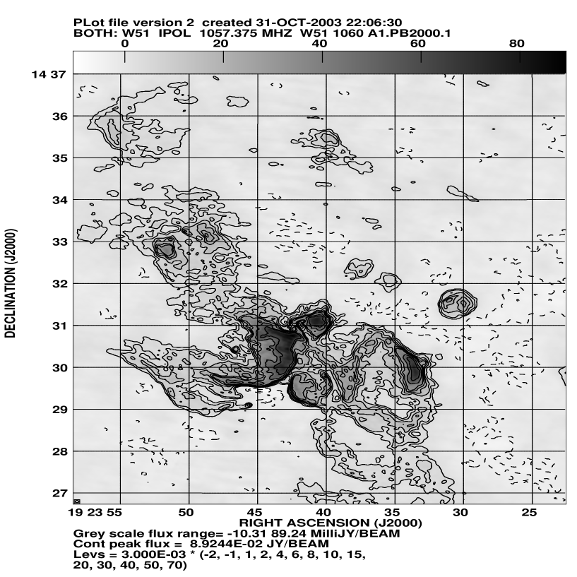
Figure 3: High resolution ($3.7^{\prime\prime}$$\times$$3.2^{\prime\prime}$ @ $82^{\circ}$) map of G49.5-0.4 at 1057MHz

While the full resolution images at 610, 1060 and 1420MHz and their analysis will be presented elsewhere, we present in Fig.3, a high resolution $3.7^{\prime\prime}$$\times$$3.2^{\prime\prime}$ image of W51A at 1060MHz. The complex nature of the region with the compact sources, shells and diffuse emission, seen in the high resolution images at 5 and 8GHz (Mehringer, 1994), are also seen in our map though with lower brightness, with the compact regions showing evidence for self absorption.

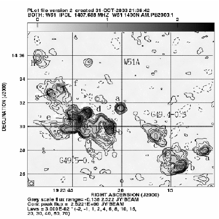
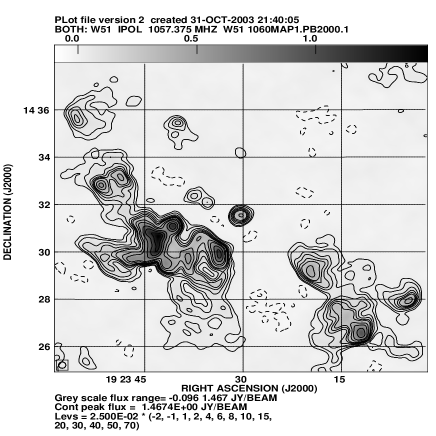
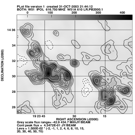
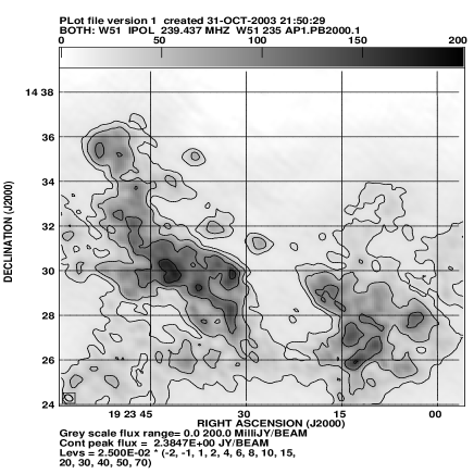
Figure 2: Maps of W51A at 1400,1060,610,240MHz made at appoximately same resolution of $20^{\prime\prime}\times 15^{\prime\prime}$. The rms noise in above maps is 12,10,6,10mJy respectively

Table 2: Observed Peak Flux Density(mJy)/beam ($I(\nu)$) for Beam of $20^{\prime\prime}$$\times$$15^{\prime\prime}$ and Integrated Flux(Jy) for HII components in W51A

Frequency	240MHz		610MHz		1060MHz		1400MHz		4860MHz*
Source	$I(\nu)$	Flux	$I(\nu)$	Flux	$I(\nu)$	Flux	$I(\nu)$	Flux	$I(\nu)$
G49.5-0.4a	66	0.27	160	0.46	440	0.93	590	1.29	530
b	120	0.79	330	1.20	1310	3.62	2060	5.11	3040
c	120	0.62	260	0.71	790	2.04	990	1.97	1130
d	36	0.42	340	0.82	1430	2.81	2210	3.24	9030
e	90	1.28	430	2.37	1750	7.97	3040	12.3	10700
f	60	0.52	180	0.62	440	1.18	480	1.26	620
g	50	0.49	200	0.55	640	1.50	740	1.42	1000
h	110	0.56	120	0.41	250	0.66	240	0.66	270
G49.4-0.3a	80		230		490		630
b	80		310		1110		1630
c	80		240		500		540

3 Measured Parameters and Physical Conditions of W51A Components

Both the components of W51A, G49.5-0.4 and G49.4-0.3, consists of several compact HII sources surrounded by diffused ionised gas (Goss & Shaver 1970, Mehringer 1994). The emission from the entire W51A region is thermal and the sources are seen to be optically thin at frequencies greater than 5GHz (Martin1972,Mehringer1994).The flux density due to continuum free-free emission from a homogeneous and isothermal spherical clouds is given by (Hjellming et al 1969)

$$S=3.07\times 10^{-2}T_{e}\ \nu^{2}\Omega(1-e^{-\tau})$$ (1)

where $S$ is integrated flux density in Jy, $T_{e}$ is electron temperature in Kelvin, $\nu$ is frequency in MHz, $\Omega$ is solid angle subtended by the source in steradians and $\tau$ is optical depth along the line of sight. At radio wavelengths, optical depth $\tau$ can be approximated as (Mezger & Henderson 1967)

$$\tau\sim 1.643\times 10^{5}\nu^{-2.1}EM\ T_{e}^{-1.35}$$ (2)

where $EM$ is emission measure in cm^-6pc and the frequency is in MHz. For resolved sources with more complex structure, the brightness as measured by the flux density per beam is the more appropriate quantity and following the procedure adopted by Wood & Churchwell (1989), we consider the value of brightness at the position of maximum intensity as the best representative of $S$/$\Omega$. In Table 2 we have listed the observed peak flux density for a gaussian beam of FWHM of $20^{\prime\prime}$$\times$$15^{\prime\prime}$.

The observed peak brightness temperature is equal to the true brightness temperature only if the source is well resolved and does not have fine structure smaller than the beam. If the source is unresolved or has fine structure, the observed peak brightness temperature is less than the true brightness temperature by an unknown factor that is determined by the ratio of the effective solid angle of the source to the solid angle of the observing beam. The main aim of high resolution observations of these sources at low frequencies is to resolve the source and get a direct estimate of the temperature of the emitting region without the uncertainty of the filling factor. The VLA observations of Mehringer (1994) and our own high resolution observations at 1400MHz suggest that many of the components are resolved with a $20^{\prime\prime}\times 15^{\prime\prime}$ beam and so could be candidates for a direct determination of the brightness temperature.

For a beam of $20^{\prime\prime}\times 15^{\prime\prime}$, the observed peak flux density per beam $S_{p}$/$\Omega_{20^{\prime\prime}\times 15^{\prime\prime}}$, estimated from the images, written as $I_{\nu}$, can be got from Eqs 1 and 2 as

$$I_{\nu}=S_{p}/\Omega_{20^{\prime\prime}\times 15^{\prime\prime}}=a\nu^{2}(1-e^{-b\nu^{-2.1}})$$ (3)

where $a=2.45\times 10^{-4}T_{e}$ , and $b=1.643\times 10^{5}EM\ T_{e}^{-1.35}$

The electron temperature $T_{e}$ and emission measure $EM$ were estimated by least-square fitting of the observed data (Table 2) into Eq.3 and the estimated $T_{e}$ and $EM$ are presented in Table 3. The plots of $S_{p}$/$\Omega_{20^{\prime\prime}\times 15^{\prime\prime}}$ against frequency for all the sources in G49.5-0.4 and G49.4-0.3 are shown in Figures 4 and 5. As is clear from the figures, in most of the sources the data agrees well with the assumption of a thermal source that is optically thick at metre wavelengths and the data is good enough to get reliable estimates of both the electron temperature and the emission measure. Some of the sources show excess emission at 240MHz. The main exception is the source G49.5-0.4h (Fig 4) which does not show an unambiguous low frequency turn over and suggests that this source is optically thin at most of the GMRT frequencies or has greatly enhanced brightness at 240MHz.

3.1 Electron Temperature

The electron temperatures for all the HII regions, as obtained from above least-square fitting, range between 2100-5600K. These temperatures are lower than expected from standard models of HII regions and from RRL studies but seem to be consistent with the literature where low frequency radio observations tend to give lower temperatures than other techniques (Shaver 1969, Kassim et al 1989 and Coppetti et al 1991). The low frequency continuum observations at 410MHz (Shaver1969) and at 151MHz (Copetti & Schmidt 1991) estimated temperatures of about 4650K and 3500K respectively for the entire W51A complex and it has been argued that these low temperatures are perhaps due to the low resolution ($>3^{\prime}$) of their observations. Subrahmanyan & Goss(1995) from their 330MHz continuum observation with $1^{\prime}$ resolution inferred that $T_{e}\sim 7800K$ for G49.5-0.4d,e components. Our estimate of $5600\pm 400$ for the temperature of G49.5-0.4e, is consistent with their direct estimate of $6200K$, based on its brightness at 330 MHz and assuming it is optically thick.

High resolution interferometric RRL studies of various HII regions in W51A have shown higher electron temperatures. H109$\alpha$ studies by van Gorkom et al(1980) found $T_{e}$ for G49.5-0.4 b,d,e sources to be 8500,6800,7400K respectively; H76$\alpha$ studies by Garay et al(1985) found 6600K and 6400K for sources d,e respectively; H96$\alpha$ observations by Mehringer(1994) found average values of $T_{e}$ around brightest components d,e in the range of 7500K and 6500K respectively. Similar values of electron temperatures have been reported from other HII regions by RRL studies; e.g. W3A: 7500 $\pm$ 750K( Roelfsema & Goss,1991), SgrA West: 7000 $\pm$500K (Roberts & Goss,1993).

The discrepancy in the temperature estimates from the RRL and the low frequency flux measurements could be explained in different ways. If the HII region has fine structure or temperature gradients, the RRL and the radio continuum emission could arise from parts of the source with different properties. The low frequency continuum emission could be probing the outer parts of the HII region which could be cooler. If there is fine structure in the source, we can invoke the filling factor $f_{w}$ ranging from 1 to 3, to explain away the discrepancy. In Table 3, we have given the filling factor $f_{w}$ required to reconcile the temperatures obtained by two techniques. However, such structure should leave some observational footprint. We have examined the high resolution maps to see if we could find some correlation between the required filling factors and other properties of the source. The sources, G49.5-0.4b,d,e, that are strongest at 5 GHz, and are the ones with the highest emission measure, are also the ones requiring the smallest filling factor corrections. The source G49.5-0.4h for which we have a lower limit on the temperature is also the largest and most relaxed component where our measured brightness temperature is most likely to reflect the true brightness. Of the components with large filling factors, G49.5-0.4a shows fine structure, having a shell like structure. The component G49.5-0.4c is not very strong and is in a complex region and so could be a blend of different components. The components G49.5-0.4(f,g) are fairly relaxed and are comparable to our beam and there is no strong reason for the high filling factor, except that they are embedded in weaker diffuse emission.

Our estimated values of the emission measure given in Table 3, are lower than those estimated from the RRL measurements. The fitting procedure gives a good estimate of the optical depth, but to convert it to emission measure one needs to know the temperature of the region. The low temperatures obtained by us using the raw fitting procedure leads to low values for the emission measure. We have recomputed the emission measures for the lowest temperature in the range given by the RRL measurements and presented these in column 5 ($EM^{\prime}$) of Table 3. These are in general agreement with the RRL emission measures.

Table 3: Derived Parameters ($T_{e},EM$) from Least-Square Fitting, RRL Temperature, Filling Factor, and Revised EM ($EM^{\prime}$)

Source	$T_{e}$(K)	$EM$	RRL $T_{e}$*(K)	$f_{w}$	$EM^{\prime}$
		(106 cm-6pc)			(106 cm-6pc)
G49.5-0.4a	2300$\pm$650	0.5$\pm$0.4	5500-7500	$>2.4$	$1.6$
b	4300$\pm$600	3.8$\pm$1.8	5000-6500	$>1.2$	$4.8$
c	3200$\pm$550	1.2$\pm$0.6	6000-7500	$>1.9$	$2.8$
d	4300$\pm$350	12.3$\pm$4.5	4500-7000	$>1.1$	$14.0$
e	5600$\pm$450	15.6$\pm$4.8	6000-8000	$>1.1$	$17.7$
f	2100$\pm$200	0.5$\pm$0.1		$>2.8$	$2.0$
g	2400$\pm$200	0.9$\pm$0.2		$>2.8$	$3.6$
h	$\geq$4900	$\geq$0.2		$>1.2$	$0.3$
G49.4-0.3a	2750$\pm$500	0.5$\pm$0.3		$>2.2$	$1.4$
b	3700$\pm$350	3.4$\pm$3.2		$>1.6$	$6.4$
c	3000$\pm$550	0.4$\pm$0.25		$>2.0$	$1.0$

Figure 4: Observed and fitted thermal spectra of HII regions in G49.5-0.4. Source h seems to be optically thin in the entire range

Figure 5: Observed and fitted thermal spectra of HII regions in G49.4-0.3.

3.2 Excess Flux at 240 MHz and a Two Components Model

In many of the components like G49.5-0.4a,b,c,f,g and all the components of G49.4-0.3, the brightness is higher at 240MHz than expected from the model fits. The possibility of flux calibration errors at 240MHz was ruled out by the general agreement of our flux density estimates of the components of W51 and 4C13.73 with the expected values based on other observations and the fact that the excess is not seen in some of the components like G49.5-0.4d,e. The physical location of the GMRT antennas being the same for all the frequencies, the 240MHz observations have better short spacing coverage than at other frequencies and so will more faithfully reproduce the extended emission. To avoid bias due to the extended emission, we have not directly used the observed peak brightness at 240MHz for the sources but have made 1-dimensional cuts in different position angles and estimated the excess of the peak brightness over the local background. While this is a bit subjective, we believe that this should reduce the possibility of systematically overestimating the brightness because of the the better short spacing coverage.

For the components with this excess flux, if we consider only the 240MHz observations, the measured brightness temperature is comparable to the RRL temperatures. However, we do not think that this a resolution of the problem of the discrepancy between the RRL and the radio continuum temperatures since this does not take into account the observations at the higher frequencies. For complex structures, it is reasonable to expect the filling factor to depend on frequency, since different parts of the source get optically thick at different frequencies. One possible explanation is to consider a spherically symmetric model with a temperature gradient, but that would require the outer regions to be hotter than the inner which may not be reasonable, since the energy source is at the centre. Another possibility is a raisin pudding model, with dense regions embedded in hot plasma. While this may not be unreasonable, the non detection of such fine structure in the high frequency, high resolution maps (Mehringer 1994) is a concern.

Rather than associating the excess flux at 240 MHz to the compact sources, one could attribute it to foreground emission that becomes strong at low frequencies. Synchrotron emission, either from the galactic foreground or from relativistic particles in the vicinity, has the property of being stronger at lower frequencies; but any smooth large scale emission of this type will not be seen by interferometric observations. If interferometric observations picks up fine structure in this emission, then a chance positional coincidence with the foreground enhancement would be required to explain the observed 240 MHz excess.

A more likely explanation is that the excess emission is due to an envelope of hot low density thermal plasma associated with the HII complex, in which all the components are embedded. This component is optically thin at all the frequencies, including 240MHz and has a flat spectrum characteristic of optically thin thermal emission. This emission adds brightness to all frequencies, but at 240MHz the emission of the optically thick inner components have fallen to low enough values for this foreground emission to be significant. For this explanation to work, the surrounding gas has to have a higher temperature than the compact components and should have structure on sufficiently small scale so that it is seen by the synthesis observations and and is not eliminated by our procedure of determining the peak brightness by taking its excess over the local mean. In the optically thin regime, we are not in a position to make independent estimates of the temperature and density of this component.

4 Summary

We have presented high resolution radio continuum images of the W51 complex made with the GMRT at 240, 610,1060 and 1400 MHz. While the 240MHz observations cover the whole complex, the higher frequency observations have focussed on the thermal component known as W51A. All the subcomponents of W51A are resolved in the $20^{\prime\prime}\times 15^{\prime\prime}$ images made at all the above frequencies. Combined with VLA observations at 5GHz with comparable resolution, the peak brightness of all the components show a well defined thermal spectrum which is optically thick at frequencies less than 1 GHz. The emission measures and the electron temperatures have been estimated by fitting the observed spectra to standard equation (Eq.3) of radiative transfer in HII regions. While the estimated values for some of the components are in reasonable agreement with the estimates from RRL observation, in many of the components, the continuum temperatures are lower than the RRL values. This suggests that even with this resolution, there are unresolved features in these components and we have estimated the filling factors required to reconcile the two measurements. The observed brightness of some of the components at 240MHz is higher than expected from the temperature predicted by the fit. This could be due to a high temperature, low emission measure envelope around the components which could be associated with the W51A complex. The discrepancies between the temperatures estimated from the continuum and the RRL observations and between continuum observations themselves suggest the need for more complex models for the HII regions including the 3-dimensional distribution of matter in the complex.

5 Acknowledgements

PKS acknowledges the support given by IUCAA under its Visiting Associate programme and by NCRA in providing its facilities.PKS also acknowledges the support given by University Grants Commission, India under Project F.8.4(74)/1999–2000/MRP.

References

- [1] Altenhoff W.J., Downes D., Pauls T., Schraml J., 1978, A&AS, 35, 23
- [2] Bieging J., 1975, in Wilson T.L., Downes D.H., eds, HII Regions and Related Topics.Springer-Verlag, Berlin, p.443
- [3] Churchwell E., Smith L.F., Mathis J., Mezger P.G., Huchtmeier W., 1978, A&A, 70, 719
- [4] Copetti M.V.F., Schmidt A.A., 1991, MNRAS, 250, 127
- [5] Garay G., Reid M.J., Moran J.M., 1985, ApJ, 289, 681
- [6] Goss W.M., Shaver P.A., 1970, Australian J. Phys, Astrophys. Suppl., 14, 1
- [7] Hjellming R.M., Andrews M.H., Sejnowski T.J., 1969, ApJ, 157, 573
- [8] Kassim N.E., Weiler K.W., Erickson W.C., Wilson T.L., 1989, Ap.J, 338, 152
- [9] Kundu M.R., Velusamy T., 1967, Ann.Astrophys., 30, 59
- [10] Martin A.H.M., 1972, MNRAS, 157, 31
- [11] Mehringer D.M., 1994, Ap.JS, 91, 713
- [12] Mezger P.G., Henderson A.P., 1967, ApJ, 147, 471
- [13] Pankonin V., Payne H.E., Terzian Y., 1979, A&A, 75, 365
- [14] Roberts D.A, Goss W.M., 1993, ApJS, 86, 133
- [15] Roelfsema P.R., Goss W.M., 1991, A&AS, 87, 177
- [16] Shaver P.A., 1969, MNRAS, 142, 273
- [17] Subrahmanyan R., Goss W.M., 1995, MNRAS, 275, 755
- [18] van Gorkom J.H., Goss W.M., Shaver P.A., Schwarz U.J., Harten R.H., 1980, A&A, 89, 150
- [19] Wilson T.L., Bieging J., Wilson W.E., 1979, A&A, 71, 205
- [20] Wilson T.L., Mezger P.G., Gardner F.F., Milne D.K., 1970, A&A, 5, 99
- [21] Wood D.O.S., Churchwell E., 1989, ApJS, 69, 831