Observational signatures of the weak lensing magnification of supernovae

Abstract

Due to the deflection of light by density fluctuations along the line of sight, weak lensing is an unavoidable systematic uncertainty in the use of type Ia supernovae (SNe Ia) as cosmological distance indicators. We derive the expected weak lensing signatures of SNe Ia by convolving the intrinsic distribution in SN Ia peak luminosity with magnification distributions of point sources. We analyze current SN Ia data, and find marginal evidence for weak lensing effects. The statistics is poor because of the small number of observed SNe Ia. Future observational data will allow unambiguous detection of the weak lensing effect of SNe Ia. The observational signatures of weak lensing of SNe Ia that we have derived provide useful templates with which future data can be compared.

I Introduction

The use of type Ia supernovae (SNe Ia) as cosmological distance indicators has become fundamental in observational cosmology (Garnavich et al., 1998; Riess et al., 1998; Perlmutter et al., 1999; Knop et al., 2003; Tonry et al., 2003; Riess et al., 2004). Although SNe Ia can be calibrated to be good standard candles (Phillips, 1993; Riess, Press, & Kirshner, 1995), they can be affected by systematic uncertainties. These include possible evolution in the intrinsic SN Ia peak brightness with time (Drell, Loredo, & Wasserman, 2000), weak lensing of SNe Ia (Kantowski, Vaughan, & Branch, 1995; Frieman, 1997; Wambsganss et al., 1997; Holz, 1998; Metcalf & Silk, 1999; Wang, 1999; Valageas, 2000; Munshi & Jain, 2000; Barber et al., 2000; Premadi et al., 2001), and possible extinction by gray dust (Aguirre, 1999).

Weak lensing effect is an unavoidable systematic uncertainty of SNe Ia as cosmological standard candles, simply because there are fluctuations in the matter distribution in our universe, and they deflect the light from SNe Ia (causing either demagnification or magnification).

In Sec.2, we derive the expected weak lensing signatures of SNe Ia by convolving the intrinsic distribution in SN Ia peak luminosity with magnification distributions of point sources. In Sec.3, we use current SN Ia data to show that weak lensing effect may have already begun to set in. Sec.4 contains a brief summary and discussions.

II Signatures of weak lensing

The observed flux from a SN Ia is

$$f=\mu L_{int},$$ (1)

where $L_{int}$ is the intrinsic brightness of the SN Ia, and $\mu$ is the magnification due to intervening matter. Note that $\mu$ and $L_{int}$ are statistically independent. The probability density distribution (pdf) of the product of two statistically independent variables can be found given the pdf of each variable (for example, see Lupton (1993)).

We find that the pdf of the observed flux $f$ is given by

$$p(f)=\int_{0}^{L_{int}^{max}}\frac{dL_{int}}{L_{int}}\,g\left(L_{int}\right)\,p\left(\frac{f}{L_{int}}\right),$$ (2)

where $g(L_{int})$ is the pdf of the intrinsic peak brightness of SNe Ia, $p(\mu)$ is the pdf of the magnification of SNe Ia. The upper limit of the integration, $L_{int}^{max}=f/\mu_{min}$, results from $\mu=f/L_{int}\geq\mu_{min}$.

A definitive measurement of $g(L_{int})$ will require a much greater number of well measured SNe Ia at low $z$ than is available at present. Since $g(L_{int})$ is not sufficiently well determined at present, we present our results for two different $g(L_{int})$’s: Gaussian in flux and Gaussian in magnitude.

The $p(\mu)$’s can be computed numerically using cosmological volume N-body simulations (see for example, Wambsganss et al. (1997); Barber et al. (2000); Premadi et al. (2001); Vale & White (2003)). We can derive the $p(\mu)$ for an arbitrary cosmological model by using the universal probability distribution function (UPDF) of weak lensing amplification Wang (1999); Wang, Holz, & Munshi (2002), with the corrected definition of the minimum convergence (Wang,Tenbarge, & Fleshman, 2004),

$$\tilde{\kappa}_{min}(z)=-\frac{3}{2}\,\frac{\Omega_{m}(1+z)}{cH_{0}^{-1}}\int_{0}^{z}dz^{\prime}\,\frac{(1+z^{\prime})^{2}}{E(z^{\prime})}\,\frac{r(z^{\prime})}{r(z)}\,[\lambda(z)-\lambda(z^{\prime})],$$ (3)

where $r(z)$ is the comoving distance in a smooth universe,

$$E(z)\equiv\sqrt{\Omega_{m}(1+z)^{3}+\Omega_{X}\rho_{X}(z)/\rho_{X}(0)+\Omega_{k}(1+z)^{2}},$$

with $\rho_{X}(z)$ denoting the dark energy density. The affine parameter

$$\lambda(z)=cH_{0}^{-1}\,\int_{0}^{z}\frac{dz^{\prime}}{(1+z^{\prime})^{2}\,E(z^{\prime})}.$$ (4)

Note that $\mu_{min}=1/(1-\tilde{\kappa}_{min})^{2}$. We have used a modified UPDF (Wang et al., 2004), with the corrected minimum convergence and extended to high magnifications. The numerical simulation data of $p(\mu)$ is converted to the modified UPDF, pdf of the reduced convergence $\eta$,

$$P(\eta)=\frac{1}{1+\eta^{2}}\,\exp\left[-\left(\frac{\eta-\eta_{peak}}{w\eta^{q}}\right)^{2}\right],$$ (5)

where $\eta=1+(\mu-1)/|\mu_{min}-1|$. The parameters of the UPDF, $\eta_{peak}$, $w$, and $q$ are only functions of the variance of $\eta$, $\xi_{\eta}$, which absorbs all the cosmological model dependence. The functions $\eta_{peak}(\xi_{\eta})$, $w(\xi_{\eta})$, and $q(\xi_{\eta})$ are extracted from the numerical simulation data. For an arbitrary cosmological model, one can readily compute $\xi_{\eta}$ Wang, Holz, & Munshi (2002), and then the UPDF (and hence $p(\mu)$) can be computed.

Fig.1 shows the prediction of the observed flux distributions of SNe Ia, with magnification distribution $p(\mu)$ given by a $\Lambda$CDM model ($\Omega_{m}$=0.3, $\Omega_{\Lambda}=0.7$) at $z=1.4$ (top panel) and $z=2$ (bottom panel) respectively. We have assumed that the intrinsic peak brightness distribution, $g(L_{int})$, is Gaussian with a rms variance of 0.193 (in units of the mean flux, and chosen to be the same as the $0.02\leq z\leq 0.1$ subset of the Riess 2004 sample).

Figure 1: Prediction of the observed flux distributions of SNe Ia for magnification distribution $p(\mu)$ given by a $\Lambda$CDM model ($\Omega_{m}$=0.3, $\Omega_{\Lambda}=0.7$) at $z=1.4$ (top panel) and $z=2$ (bottom panel) respectively. We have assumed that the intrinsic peak brightness distribution, $g(L_{int})$, is Gaussian with a rms variance of 0.193 (in units of the mean flux).

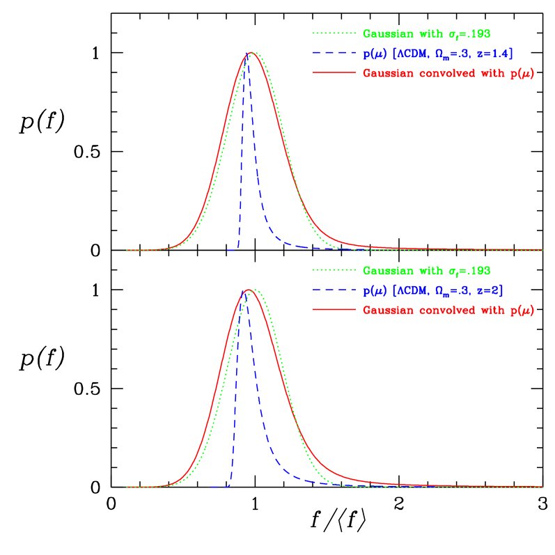
Fig.2 is the same as Fig.1, except here we have assumed that $g(L_{int})$ is Gaussian in magnitude, with a rms variance of 0.213 mag (chosen to be the same as the $0.02\leq z\leq 0.1$ subset of the Riess 2004 sample).

Figure 2: Same as Fig.1, except here we have assumed that the intrinsic peak brightness distribution, $g(L_{int})$, is Gaussian in magnitude, with a rms variance of 0.213 mag.

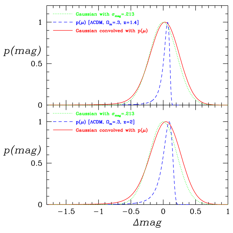
Clearly, there are two signatures of the weak lensing of SNe Ia in the observed brightness distribution of SNe Ia. The first signature is the presence of a non-Gaussian tail at the bright end, which is due to the high magnification tail of the magnification distribution. The second signature is the slight shift of the peak toward the faint end (compared to the pdf of the intrinsic SN Ia peak brightness), which is due to $p(\mu)$ peaking at $\mu<1$ (demagnification) because the universe is mostly empty. As the redshift of the observed SNe Ia increases, the non-Gaussian tail at the bright end will grow larger, while the peak will shift further toward the faint end (see Figs.1-2).

If the distribution of the intrinsic SN Ia peak brightness is Gaussian in flux, the dominant signature of weak lensing is the presence of the high magnification tail in flux. If the distribution of the intrinsic SN Ia peak brightness is Gaussian in magnitude, the dominant signature of weak lensing is the shift of the peak of observed magnitude distribution toward the faint end due to demagnification. This is as expected, since the magnitude scale stretches out the distribution at small flux, and compresses the distribution at large flux.

III Evidence of weak lensing in current supernova data

We use the Riess sample (Riess et al., 2004) to explore possible weak lensing in current SN Ia data, as this sample contains the largest number of SNe Ia at $z>1$ that are publicly available.

Our high $z$ subset consists of 63 SNe Ia from the Riess sample with with $0.5\leq z\leq 1.4$. Our low $z$ subset consists of 47 SNe Ia from the Riess sample with $0.02\leq z\leq 0.1$. Table 1 shows the redshift distribution of the 63 SNe Ia in the high $z$ subset. To enable meaningful comparison of the high $z$ and low $z$ samples, the bestfit cosmological model has been subtracted from the brightnesses of all the SNe Ia in both samples. The bestfit cosmological model (found by allowing the dark energy density to be a free function given by 4 parameters) has been obtained via flux-averaging of the gold set of 157 SNe Ia of the Riess sample, combined with CMB and galaxy survey data Wang & Tegmark (2004), hence it should have very weak dependence on the mean brightnesses of the low $z$ and high $z$ SN Ia samples.

Table 1

Redshift distribution of SNe Ia in the high $z$ subset

$z$	[.5, .7]	[.7, .9]	[.9, 1.4]
number	27	21	15

Fig.3 shows the flux distributions of 63 SNe Ia with $0.5\leq z\leq 1.4$ (top panel) and 47 SNe Ia with $0.02\leq z\leq 0.1$ (bottom panel). The bestfit cosmological model obtained by Wang & Tegmark (2004) using flux-averaging (which minimizes weak lensing effect, see Wang (2000b); Wang & Mukherjee (2004)) has been subtracted.

Figure 3: The flux distributions of 63 SNe Ia with $0.5\leq z\leq 1.4$ (top panel) and 47 SNe Ia with $0.02\leq z\leq 0.1$ (bottom panel). The bestfit model obtained by Wang & Tegmark (2004) using flux-averaging (which minimizes weak lensing effect) has been subtracted. Clearly, the distribution of the low $z$ SNe Ia is consistent with Gaussian, while the high $z$ SNe Ia seem to show both signatures of weak lensing (high magnification tail and demagnification shift of the peak to smaller flux). The error bars indicate the Poisson noise of the weak lensing prediction (solid curve).

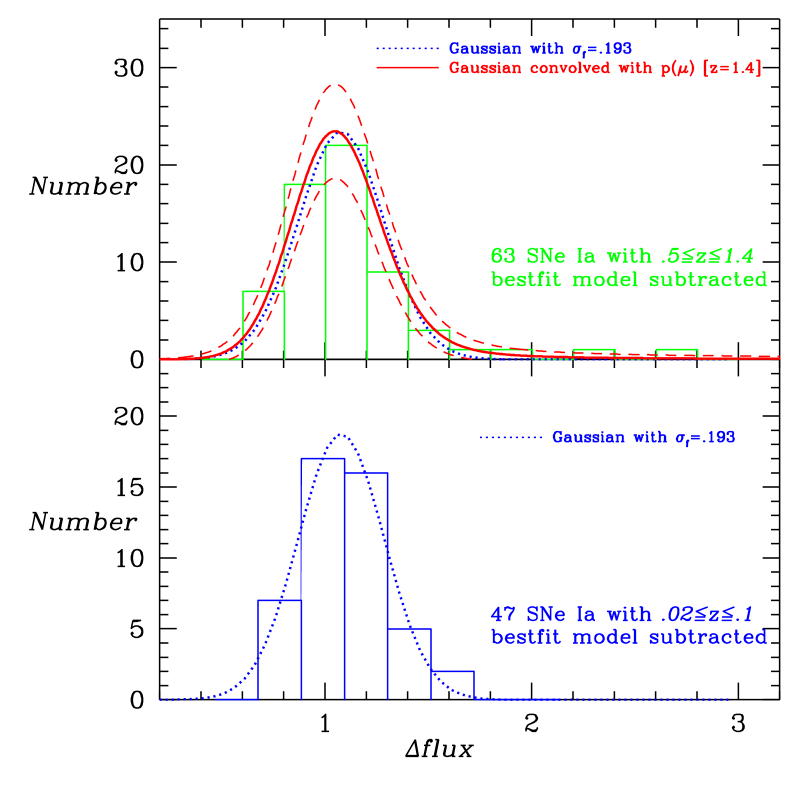
Fig.4 is the same as Fig.3, except here we have fitted the distribution of the low $z$ SNe Ia to a Gaussian in magnitude, and have binned the high $z$ SNe Ia in magnitude as well for comparison.

Figure 4: Same as Fig.3, except here we have fitted the distribution of the low $z$ SNe Ia to a Gaussian in magnitude, and have binned the high $z$ SNe Ia in magnitude as well for comparison.

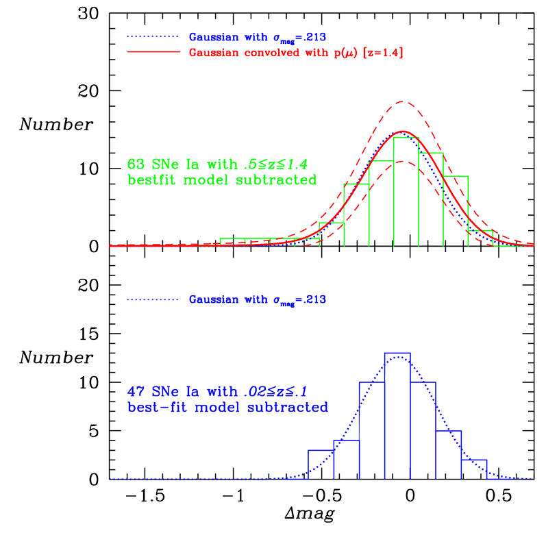
The top panels of Figs.3 and 4 show the predicted distributions of SN Ia peak brightness, obtained by convolving the bestfit Gaussian distribution at low $z$ (dotted line) with $p(\mu)$ for the bestfit cosmological model with $z=1.4$ (solid line), and the Poisson noise expected from the finite number of SNe Ia in each bin (dashed lines).

Clearly, the distribution of the low $z$ SNe Ia is consistent with Gaussian in both flux and magnitude, while the high $z$ SNe Ia seem to show both signatures of weak lensing: the high magnification tail at bright end and the demagnification shift of the peak toward the faint end. Within the uncertainties of the Poisson noise, the flux and magnitude distributions of the high $z$ SNe Ia are roughly consistent with the upper bound set by the maximal expected amount of weak lensing in the best fit model.

Both the presence of the bright end tail and the shift of the peak toward the faint end are more pronounced than the predictions based on standard lensing magnifications (see Figs.3-4). However, since the number of SNe Ia at high $z$ is still small, the difference may have resulted from statistical fluctuations (Poisson noise).

Table 2 compares the high $z$ and low $z$ SNe Ia plotted in Figs.3 and 4. The mean brightness and skewness of the distributions have been calculated for both flux and magnitude distributions. The rms variance of the skewness $S_{3}$ for a Gaussian distribution is $\sigma_{S_{3}}^{G}\simeq\sqrt{6/N}$ (Press et al., 1994), where $N$ is the number of SNe Ia in the subset.

Table 2

Comparison of high $z$ and low $z$ SNe Ia

$z$ of SNe	$\langle f\rangle^{a}$	$S_{3}\pm\sigma_{S_{3}}^{G}$(flux)	$\langle mag\rangle^{b}$	$S_{3}\pm\sigma_{S_{3}}^{G}$(mag)
$.5\leq z\leq 1.4$	1.115	$2.12\pm 0.31$	$-.0763$	$-1.06\pm 0.31$
$.5\leq z\leq 1.4^{c}$	1.055	$0.66\pm 0.32$	$-.0352$	$-0.25\pm 0.32$
$.02\leq z\leq.1$	1.096	$0.60\pm 0.36$	$-.0805$	$-0.19\pm 0.36$

^a in units of the flux in the bestfit cosmological model obtained via flux-averaging in Wang & Tegmark (2004).
^b defined to be $-2.5\log(flux)$, where $flux$ is the dimensionless flux defined above.
^c excluding the three brightest SNe listed in Table 3.

The high $z$ and low $z$ SNe Ia differ little in mean brightness; this is as expected since the bestfit cosmological model obtained using the gold set of 157 SNe Ia of the Riess sample (together with CMB and galaxy clustering data) has been subtracted. In the absence of weak lensing, one would expect that the low $z$ and high $z$ SN Ia samples have similar distributions, hence similar values of the skewness $S_{3}$. If the intrinsic distribution of SN Ia brightnesses were Gaussian in flux (magnitude), one would expect $S_{3}=0\pm\sigma_{S_{3}}^{G}$ for the data in flux (magnitude). Table 2 shows that: (1) The high $z$ SN Ia sample has a significantly larger skewness $S_{3}$ (for both flux and magnitude distributions) than the low $z$ sample; (2) The large skewness of the high $z$ sample is primarily due to the three brightest SNe Ia. Both these points are consistent with the signatures of weak lensing discussed in Sec.2.

Table 3 lists the three brightest SNe Ia in the bright end tails of Figs.3 and 4. All three SNe Ia are in the “gold” sample of Riess et al. (2004). The last column in Table 3 lists the possible range of magnification $\mu$ for each SN Ia, [$(f-df)/\langle f\rangle$, $(f+df)/\langle f\rangle$], with $df/f=\sinh\left(\sigma_{\mu_{0}}\ln 10/2.5\right)$, and $\langle f\rangle$ given by the low $z$ subset. Note that the possible magnification of SN1998I has a very large uncertainty, because its distance modulus has a very large uncertainty in the Riess sample: $\mu_{0}=42.91\pm 0.81$, which correspond to a flux uncertainty of about 80%.

Table 3

Three brightest SNe Ia

SN	$z$	$\mu_{0}$	$\sigma_{\mu_{0}}$	possible $\mu$
SN1997as	0.508	41.64	0.35	[1.42, 2.78]
SN2000eg	0.540	41.96	0.41	[1.10, 2.50]
SN1998I	0.886	42.91	0.81	[0.44, 4.40]

Note that the bestfit cosmological model Wang & Tegmark (2004) was obtained using the gold set of 157 SNe Ia of the Riess sample Riess et al. (2004), flux-averaged and combined with CMB and galaxy clustering data. The mean brightnesses of the low $z$ and high $z$ samples considered in this paper were not used in deriving the bestfit cosmological model (which is given by 6 parameters). The fact that the low $z$ and high $z$ samples have about the same mean brightnesses shows the validity of the bestfit cosmological model, since weak lensing does not change the mean brightness of teh high $z$ sample due to flux conservation.

The second row in Table 2 shows that if we exclude the three brightest SNe listed in Table 3, the skewness of the high $z$ sample drops to about the same as that of the low $z$ sample. However, the mean brightness of the high $z$ sample drops below that of the low $z$ sample, such that the high $z$ sample is about 4% fainter in flux than the low $z$ sample. This suggests that the three brightest SNe in the high z sample are probably not outlyers, but may belong to the high magnification tail of $p(\mu)$.

Finally, we do a Kolmogorov-Smirnov test to assess whether the low $z$ and high $z$ SNe Ia could be from the same brightness distribution (i.e., no weak lensing of the high $z$ sample). Table 4 shows the Kolmogorov-Smirnov test of the low $z$ versus high $z$ SN Ia sample, and the high $z$ SN Ia sample compared to a Gaussian in magnitude (with $\sigma_{mag}=0.213$) convolved with $p(\mu)$ at $z=1.4$ (as plotted in Fig.4a). We have chosen the later distribution for comparison with the high $z$ sample, because the low $z$ sample appears slightly more Gaussian in magnitude (with smaller $S_{3}$, see Table 2).

Table 4

Kolmogorov-Smirnov test

subtracted cosmological model	bestfit model		($\Omega_{m}=0.27$, $\Omega_{\Lambda}=0.73$)
	D	prob.	D	prob.
low $z$ and high $z$ sample	0.153	0.522	0.184	0.291
high $z$ sample and $p(mag)^{a}$	0.096	0.585	0.104	0.482

^a a Gaussian in magnitude (with $\sigma_{mag}=0.213$) convolved with $p(\mu)$ at $z=1.4$, see Eq.(2).

The Kolmogorov-Smirnov test gives $D$, the maximum value of the absolute difference between two cumulative distribution functions, and $prob$, the probability that $D>observed$. Small values of $prob$ show that the two distributions are significantly different. Table 4 shows that current data do not yield results of high statistical significance, however, the high $z$ SN Ia sample is more consistent with a lensed distribution than with the low $z$ SN Ia sample. Changing the subtracted cosmological model from the bestfit model to a popular model with $\Omega_{m}=0.27$, $\Omega_{\Lambda}=0.73$ does not change our results qualitatively.

IV Summary and Discussion

We have derived the expected weak lensing signatures of SNe Ia in the distribution of observed SN Ia peak brightness, the presence of a high magnification tail at the bright end of the distribution, and the demagnification shift of the peak of the distribution toward the faint end (see Figs.1-2).

Our method is complementary to that of Metcalf (2001); Williams & Song (2004); they use the correlation between foreground galaxies and supernova brightnesses to detect weak lensing, while our method only uses the statistics of supernova brightnesses and does not depend on the observation of foreground galaxies.

We have compared 63 high $z$ SNe Ia ($0.5\leq z\leq 1.4$) with 47 low $z$ SNe Ia ($0.02\leq z\leq 0.1$) from the Riess sample (Riess et al., 2004). We find that the observed flux and magnitude distributions of the high $z$ sample are roughly consisitent with the maximal expected amount of weak lensing magnification (see Figs.3-4), within the Poisson noise due to the small number of SNe Ia in each bin.

We have identified the three brightest SNe Ia in the high $z$ subset ($0.5\leq z\leq 1.4$) of the Riess sample, and estimated a possible range of magnification for each SN Ia (Table 3). Observational follow-up of the regions near these SNe Ia may show whether these SNe Ia have indeed been magnified. Note that selection effects should not be important here, since the three brightest SNe are at intermediate redshifts (where the fainter SNe are not close to the detection limits of the surveys).

Our results are consistent with those of Williams & Song (2004); Bassett & Kunz (2004). Williams & Song (2004) found that brighter SNe Ia are preferentially found behind regions which are overdense in foreground galaxies, as expected in weak lensing. Bassett & Kunz (2004) found tentative evidence for a deviation from the reciprocity relation between the angular diameter distance and the luminosity distance, which could be due to the brightening of SNe Ia due to lensing.

Although the observed flux/magnitude distribution of the high $z$ SN Ia sample deviates from a Gaussian in ways that are qualitatively consisitent with the weak lensing effects (allowing for Poisson noise), it is possible that these deviations could be due to other unidentified systematic effects. However, it is important to note that if we remove the three brightest SNe Ia in the high $z$ sample, the distributions become more Gaussian, but the mean becomes biased (see Table 2). Therefore, these three SNe Ia might not be outliers, and should be included in the data analysis.

Fortunately, the non-Gaussianity of the high $z$ SN Ia flux/magnitude distribution (regardless of its origin – weak lensing or some other systematic effect) does not seem to alter the mean of the distribution (compared to the low $z$ sample). This means that we can, and should, use flux averaging in order to obtain unbiased estimates of cosmological parameters (Wang, 2000b; Wang & Mukherjee, 2004).

Our results explain the difference between the cosmological constraints found by Riess et al. (2004) and Wang & Tegmark (2004) for the same model assumptions (see Fig.10 of Riess et al. (2004) and Fig.2(a) of Wang & Tegmark (2004)). Wang & Tegmark (2004) used flux-averaging in their likelihood analysis; Riess et al. (2004) did not.

As more SNe Ia are discovered at high $z$, it becomes increasingly important to minimize the effect of weak lensing (or other non-Gaussian systematic effects that conserve flux) by flux-averaging (Wang, 2000b; Wang & Mukherjee, 2004) in using SNe Ia to probe cosmology.

It seems that weak lensing effects, or some other systematic effect that mimics weak lensing qualitatively, may have begun to set in (see Figs.3-4 and Tables 2 & 4). However, the statistics is poor because of the small number of observed SNe Ia. Future observational data from current and planned SN Ia surveys will allow unambiguous detection of the weak lensing effect of SNe Ia. The observational signatures of weak lensing of SNe Ia that we have derived (see Figs.1-2) provide useful templates with which future data can be compared.

Public software: A Fortran code that uses flux-averaging statistics to compute the likelihood of an arbitrary dark energy model (given the SN Ia data from Riess et al. (2004)) can be found at $http://www.nhn.ou.edu/\sim wang/SNcode/$.