Data reduction methods for single-mode optical interferometry

The interferometric data processing methods that we describe in this paper use a number of innovative techniques. In particular, the implementation of the wavelet transform allows us to obtain a good immunity of the fringe processing to false detections and large amplitude perturbations by the atmospheric piston effect, through a careful, automated selection of the interferograms. To demonstrate the data reduction procedure, we describe the processing and calibration of a sample of stellar data from the VINCI beam combiner. Starting from the raw data, we derive the angular diameter of the dwarf star $\alpha$ Cen A. Although these methods have been developed specifically for VINCI, they are easily applicable to other single-mode beam combiners, and to spectrally dispersed fringes.

1 Introduction

Although interferometric techniques are now used routinely around the world, the processing of interferometric data is still the subject of active research. In particular, the corruption of the interferometric fringes by the turbulent atmosphere is currently the most critical limitation to the precision of the ground-based interferometric measurements.

Installed at the Very Large Telescope Interferometer (VLTI), the VINCI instrument coherently combines the infrared light coming from two telescopes in the infrared $H$ and $K$ bands. The first fringes were obtained in March 2001 with the VLTI Test Siderostats, and in October 2001 with the 8m Unit Telescopes (UTs). To reduce the large quantity of data produced by this instrument, we have developed innovative interferometric data analysis methods, using in particular the wavelet transform. We have appplied them successfully to a broad range of interferometric observations obtained with very different configurations of the VLTI (0.35 m siderostats, 8 m Unit Telescopes, 16 m to 140 m baselines, $K$ and $H$ band observations).

Since the first fringes of VINCI, more than 800 nights of observations have been conducted with this instrument. This allowed us to record a large number of individual star observations, under extremely different atmospheric and instrumental conditions. The data processing methods that are described in the present paper were successfully applied to all these configurations, and consistently provided reliable and precise results. This gives us good confidence that they are efficient and robust, and can be generalized to other interferometric instruments.

Our goal in this paper is to give a step by step description of the processing of the VINCI data, from the raw data to the calibrated visibility. To illustrate this processing, we selected from the commissioning data a series of observations of a bright star and its calibrator, $\alpha$ Cen A and $\theta$ Cen respectively (Sect. 3). A complete overview of the data analysis work flow is presented in Fig. 1. It can be used as a reference to follow the logical progression of this paper. The photometric calibration of the interferograms is described in Sect. 4 and 5. The criteria for the selection of the interferograms are detailed in Sect. 6, and the computation of the visibility values and associated errors is given in Sect. 7. A number of quality controls is applied to the reduced data; they are described in Sect. 8. The calibration of the visibility is illustrated in Sect. 9. We demonstrate in particular the computation of the statistical and systematic errors on the visibility values.

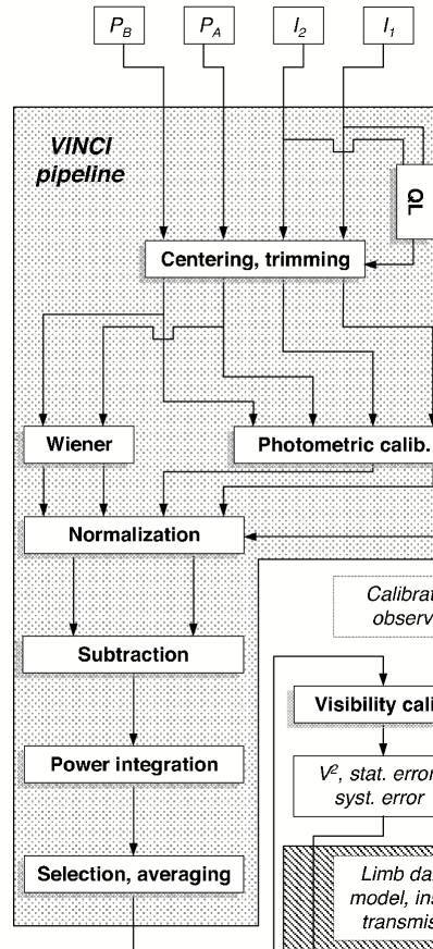
Figure 1: Overview of the VINCI data analysis work flow. The shaded area delimits the processing executed automatically by the instrument data pipeline. The hatched area (lower right) covers the astrophysical interpretation of the measured visibility, not adressed in the present paper.

2 Instrument description

2.1 The VLT Interferometer and VINCI

The Very Large Telescope Interferometer (VLTI, Glindemann et al. glindemann (2000); Glindemann et al. 2003a ; Glindemann et al. 2003b ; Schöller et al. schoeller03 (2003)) has been operated by the European Southern Observatory on top of the Cerro Paranal, in Northern Chile since March 2001. In its current state of completion, the light coming from two telescopes can be combined coherently in VINCI, the VLT Interferometer Commissioning Instrument (Fig. 2), or in the MIDI instrument (Leinert et al. leinert00 (2000)). In December 2002, MIDI obtained its first fringes at $\lambda=8.7\,\mu$m between the two 8m Unit Telescopes Antu (UT1) and Melipal (UT3). Another instrument, AMBER (Petrov et al. petrov00 (2000)) will soon allow the simultaneous recombination of three telescope beams (its first observations are scheduled for 2004).

Figure 2: View of the VINCI instrument installed in the VLTI interferometric laboratory. The MONA beam combiner is the visible above the center of the image (white box), with its optical fiber inputs and outputs. The beams coming from the VLTI Delay Lines enter the optical table from the bottom of the picture. Figure not available on the astro-ph version.

Figure 3: Principle of the VINCI instrument. Figure not available on the astro-ph version.

A detailed description of the VINCI instrument, including its hardware and software design, can be found in Kervella et al. (kervella00 (2000)). Fig. 3 shows the setup of VINCI. The two beams enter the instrument from the bottom of the figure, after having been delayed by two optical delay lines (Derie derie00 (2000)). Once the stellar light from the two telescopes has been injected into the optical fibers (injections A and B), it is recombined in the MONA triple coupler. VINCI is based on the same principle as the FLUOR instrument (Coudé du Foresto et al. coude98 (1998)), and recombines the light through single-mode fluoride glass optical fibers that are optimized for $K$ band operation ($\lambda=2.0-2.4\ \mu$m). It uses in general a regular $K$ band filter, but can also observe in the $H$ band ($\lambda=1.4-1.8\ \mu$m) using an integrated optics beam combiner (Berger et al. berger01 (2001)). The first observations with this new generation coupler installed at the VLTI focus have given promising results (Kervella et al. 2003a ; Kern et al. kern03 (2003)).

2.2 Beam combination

The central element of VINCI is its optical correlator (MONA), based on single-mode fluoride glass fibers and couplers. It was designed and built specifically for VINCI by the company Le Verre Fluoré (France). The waveguides are used to filter out the spatial modes of the atmospheric turbulence. In the couplers, the fiber cores are brought very close to each other (a few $\mu$m) and the two electric fields interfere directly with each other by evanescent coupling of the electromagnetic waves. Motorized polarization controllers allow the matching of the beam polarizations, in order to obtain the best possible interferometric transfer function.

The general principle of the MONA box is shown in Fig. 4. MONA contains three couplers: two side couplers (that provide two photometric outputs $P_{A}$ and $P_{B}$ to monitor the efficiency of the stellar light injection in the optical fibers) and a central coupler that is used for the beam combination. The latter provides two complementary interferometric outputs $I_{1}$ and $I_{2}$. The four output fibers are eventually arranged on a 125 $\mu$m square and imaged onto an infrared camera (LISA), built around a HAWAII detector. Only four small windows, of one pixel each, are read from the detector to increase the frame frequency and reduce the readout noise.

The Optical Path Difference (OPD) between the two beams is modulated by a mirror mounted on a piezo translator. This modulation allows one to sweep through the interference fringes (at zero OPD), that appear as temporal modulations of the $I_{1}$ and $I_{2}$ intensities on the detector. While the OPD is scanned, the four output signals are sampled at a few kHz. The four resulting time sequence signals (two photometric and two interferometric) are then available for processing. The interferogram acquisition rate can be set between 0.1 Hz (faint objects) and 20 Hz (bright targets).

Figure 4: Principle of the MONA beam combiner. Figure not available on the astro-ph version.

2.3 Coherencing

During the observations, a simple fringe packet centroiding algorithm is applied in near real-time to the raw data. The fringe packet center is localized with a precision of about one fringe (2 $\mu$m) after each scan and the resulting error is fed back to the VLTI delay lines as an OPD offset. This capability, called fringe coherencing, ensures that the residual OPD is less than a coherence length despite possible instrumental drifts. Still, the correction rate (once per scan, i.e. a few Hz) is too slow to remove the differential piston mode of the turbulence. A fringe tracking unit is anticipated for the VLTI (FINITO, Gai et al. gai03 (2003)) that will remove the differential piston and stabilize the interference pattern at the sub-fringe level (fringe cophasing), thus enabling longer integration times for the scientific instrument.

3 The selected sample data sets

3.1 Targets

To illustrate the processing of the VINCI data on representative files, we have chosen two series of interferograms obtained respectively on a calibrator star, $\theta$ Cen, and a target of scientific interest, $\alpha$ Cen A, on the intermediate length E0-G1 baseline (66 m ground length). $\theta$ Cen was chosen from the Cohen et al. (cohen99 (1999)) catalogue. These authors compiled a grid of calibrator stars whose angular diameter is typically known with a relative precision better than 1%. Bordé et al. (borde02 (2002)) recently revised this catalogue specifically for its application to long baseline interferometry.

The observations of $\alpha$ Cen A and $\theta$ Cen discussed here were carried out with the two 0.35 m test siderostats of the VLTI. Both stars are bright, but $\theta$ Cen is significantly smaller than $\alpha$ Cen A, therefore its visibility is higher. The relevant properties of $\theta$ Cen and $\alpha$ Cen are reported in Table 1. The angular diameter of $\alpha$ Cen A was measured for the first time by Kervella et al. (2003b ), based on a series of observations that include the two data sets discussed here.

The file names and characteristics of the two selected data sets are given in Table 2, to allow the interested reader to retrieve them from the ESO Archive (http://archive.eso.org/).

Table 1: Relevant parameters of $\theta$ Cen and $\alpha$ Cen A.

	$\theta$ Cen	$\alpha$ Cen A
	HD 123139	HD 128620
$m_{\mathrm{V}}$	2.1	-0.0
$m_{\mathrm{K}}$	-0.1	-1.5
Spectral Type	K0IIIb	G2V
$\rm T_{\mathrm{eff}}$ (K)a	4980	5790
$\log g^{\mathrm{a}}$	2.75	4.32
$[{\rm Fe}/{\rm H}]^{\mathrm{a}}$	0.03	0.20
$\theta_{\rm{UD}}$ (mas)b	5.305 $\pm$ 0.020	8.314 $\pm$ 0.016

• $\rm T_{\mathrm{eff}}$, $\log g$ and $[{\rm Fe}/{\rm H}]$ from Cayrel de Strobel et al. (cayrel01 (2001)) and Morel et al. (morel00 (2000)), respectively for $\theta$ Cen and $\alpha$ Cen A.

• Measured diameters from Kervella et al. (2003b ).

3.2 Acquisition parameters and data structure

Following the standard procedure used with VINCI, a series of 500 interferograms was obtained on each object. The two data sets were taken on July 15, 2002, starting at UT times 01:32:32 for $\theta$ Cen, and 02:33:09 for $\alpha$ Cen A. The piezo mirror scanning speed was set to 650 $\mu$m/s, giving a fringe frequency of 297 Hz. This intermediate speed is used commonly for the operation of VINCI with the VLTI Test Siderostats. The LISA camera frequency was set to 1.5 kHz in order to obtain a sampling of 5 points per fringe. The choice of the scanning speed (hence the sampling rate of the camera) is the result of a compromise between the photometric SNR and the phase perturbations of the atmosphere (dominant at low scanning speed). The VINCI instrument allows one to scan up to a fringe frequency of 680 Hz (camera frequency of 3.4 kHz). This extreme speed is useful in the case of observations with the 8 m Unit Telescopes to reduce the influence of the photometric fluctuations on the interference fringes (multi-speckle regime). Fig. 5 shows the raw signals of one interferogram obtained on $\theta$ Cen. This is the second scan in the series of 500, and it is of average quality in terms of injected flux stability. The photometric fluctuations are clearly visible in all four channels, while the interference fringes are located close to the center of the scan. The fringes are naturally in phase opposition between the two channels $I_{1}$ and $I_{2}$.

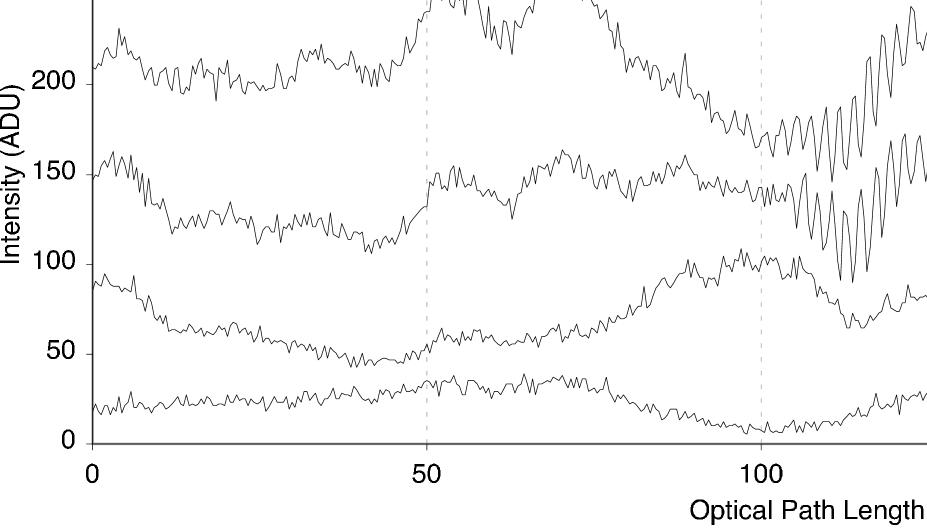
Figure 5: The raw signals $I_{1}$, $I_{2}$, $P_{A}$ and $P_{B}$, for one interferogram obtained on $\theta$ Cen. The original signals have been translated vertically respectively by +90, +40, +40 and 0 ADUs for clarity.

Each star observation consists of four files (batches), that each contain a series of acquisitions (scans) of the four signals coming out of MONA, with four different configurations of the instrument. The first three batches are used for the calibration of the camera background and instrument transmission, and usually contain 100 scans. The fourth batch contains the fringes. They are recorded in the following sequence:

1. Off-source: the two injection parabolas of VINCI are displaced in order to remove the star image from the single-mode fiber head.

2. Beam A: the A injection parabola is brought back to the position where the star light is injected in the optical fiber, while B is still off.

3. Beam B: symmetrically, only the beam B is injected in the MONA beam combiner, while A is off. The Beam A and Beam B sequences are used in the computation of the $\kappa$ matrix (Sect. 4.1).

4. On-source: both beams are injected into MONA, and interference can occur. This last series usually contains 500 scans and is used to compute the squared coherence factor $\mu^{2}$ (the interferometric observable, defined in Sect. 6.2).

Table 2: Sample data sets. $N$ is the number of scans.

File name	Target	Type	$N$
VINCI.2002-07-15T01:30:12.042	$\theta$ Cen	Off	100
VINCI.2002-07-15T01:30:53.273	$\theta$ Cen	A	100
VINCI.2002-07-15T01:31:36.505	$\theta$ Cen	B	100
VINCI.2002-07-15T01:32:31.645	$\theta$ Cen	On	500
VINCI.2002-07-15T02:30:49.318	$\alpha$ Cen A	Off	100
VINCI.2002-07-15T02:31:30.046	$\alpha$ Cen A	A	100
VINCI.2002-07-15T02:32:10.840	$\alpha$ Cen A	B	100
VINCI.2002-07-15T02:33:08.661	$\alpha$ Cen A	On	500

4 Preliminary steps

4.1 Computation of the $\kappa$ matrix

To properly calibrate the photometric fluctuations of the interferometric signals I₁ and I₂ using the two photometric outputs P_A and P_B, it is necessary to know precisely the coefficients linking the intensities of these four outputs. The relationships between the four channels can be approximated, within a very good precision (Coudé du Foresto et al. cdf97 (1997)), by the following expressions:

$${I}_{1}=\kappa_{1,A}\ {P}_{A}+\kappa_{1,B}\ {P}_{B}$$ (1)

$${I}_{2}=\kappa_{2,A}\ {P}_{A}+\kappa_{2,B}\ {P}_{B}$$ (2)

The $\kappa$ coefficients correspond to the differential gains between the four channels of VINCI. They include the coupling ratios of the MONA box, the coupling efficiency of each fiber to the physical pixels of the infrared camera, and the differential quantum efficiency between these pixels. Due to the chromatic transmission of the couplers, the color of the observed object plays a role in the $\kappa$ coefficients, and they also tend to evolve due to the slow motion of the fiber spots on the LISA detector. It is therefore necessary to measure these coefficients (the $\kappa$ matrix) immediately before each star observation. Each pair of $\kappa$ coefficients is computed simultaneously using a classical $\chi^{2}$ minimization algorithm with two variable parameters. The errors on the estimation of the $\kappa$ coefficients are derived from the residual dispersion of the measurement points around the linear model.

Table 3 gives the $\kappa$ coefficients derived for the $\theta$ Cen and $\alpha$ Cen observations. The small differences between the $\kappa$ values for the two stars may come from the slightly different colors of these objects, or from a small variation of the alignment of the output spots on the LISA infrared camera pixels between the two observations (they are separated in time by $\Delta t\simeq 1$ h).

Ideally, the $\kappa$ coefficients should be balanced between the four outputs in order to maximize the efficiency of the interference, and simultaneously to give high SNR photometric signals for the calibration of the interferograms. The observed inbalance (that can reach up to a factor 5 in the selected sample batches) is due to the fact that the unexpectedly fast aging of the three optical couplers in the MONA box has increased significantly their sensitivity to temperature. This effect cannot be corrected on the coupler itself, and causes a slow (timescale of months) but large amplitude evolution of the $\kappa$ matrix. Due to the very different time scales of these variations (months) and of the scientific observations (hours), this sensitivity is expected to have no significant impact on the observations other than a uniform and moderate reduction of the quality of the LISA signals.

Table 3: $\kappa$ coefficients measured for $\theta$ Cen and $\alpha$ Cen A.

	$\theta$ Cen	$\alpha$ Cen A
$\kappa_{1A}$	$0.7569\pm 0.0061$	$0.7576\pm 0.0037$
$\kappa_{1B}$	$4.1231\pm 0.0160$	$4.1877\pm 0.0120$
$\kappa_{2A}$	$1.3089\pm 0.0054$	$1.2790\pm 0.0044$
$\kappa_{2B}$	$2.4855\pm 0.0143$	$2.4735\pm 0.0061$

4.2 Fringe localization

The first step of the processing is to trim the long interferogram to restrict it to a shorter segment, where the fringes are centered. The detection of the fringes is then achieved with the Quicklook signal QL, that is computed using the simple formula:

$${QL}={I}_{1}-a\ {I}_{2}$$ (3)

where $a$ is given by

$$a=\frac{\sum_{i=1}^{N}{{I}_{1}(i)\ {I}_{2}(i)}}{\sum_{i=1}^{N}{{I}_{1}^{2}(i)}}$$ (4)

where $N$ is the number of samples of the raw signals $I_{1}$ and $I_{2}$. This operation attenuates the photometric fluctuations and increases the SNR of the fringes. Once the fringes are localized precisely by detecting the maximum of the wavelet power spectral density (WPSD) of the QL, the four raw signals are trimmed accordingly. If the fringes have been found too close to the edge of the interferogram, the scan is discarded to avoid any bias of the data. In addition, if a large amplitude jump of the position of the fringe packet is detected between two consecutive scans (more than 20 $\mu$m), a strong piston effect is suspected and the scan is rejected (see also Sect. 6).

5 Photometric calibration

5.1 General principle

The photometric calibration of the interferograms produced by VINCI is achieved using the two photometric control signals P_A and P_B and the $\kappa$-matrix. The calibration is computed separately for the I₁ and I₂ channels using the following formulae (see Coudé du Foresto et al. cdf97 (1997) for their derivation):

$$I_{1\,cal}=\frac{1}{2\ \sqrt{\kappa_{1,A}\ \kappa_{1,B}}}\frac{I_{1}-\kappa_{1,A}P_{A}-\kappa_{1,B}P_{B}}{[\sqrt{P_{A}\ P_{B}}]_{\mathrm{Wiener}}}$$ (5)

$$I_{2\,cal}=\frac{1}{2\ \sqrt{\kappa_{2,A}\ \kappa_{2,B}}}\frac{I_{2}-\kappa_{2,A}P_{A}-\kappa_{2,B}P_{B}}{[\sqrt{P_{A}\ P_{B}}]_{\mathrm{Wiener}}}$$ (6)

The subscript “Wiener” designates optimally filtered signals (Sect. 5.2). This process allows one first to subtract the photometric fluctuations that were introduced in the interferometric channels by the turbulent atmosphere (calibration), and then to normalize the resulting signals to the geometrical mean of the two photometric channels $P=\sqrt{P_{A}\ P_{B}}$. As an example of calibration, the subtraction of $\kappa_{1,A}P_{A}+\kappa_{1,B}P_{B}$ from the original $I_{1}$ is presented in Fig. 6. The Wiener filtering of $P$, essential to avoid numerical instabilities, is described in the next paragraph (Sect. 5.2). After the normalization, $I_{1\ {\rm cal}}$ and $I_{2\ {\rm cal}}$ are apodized at their extremities, to prevent any edge effect during the numerical wavelet transform.

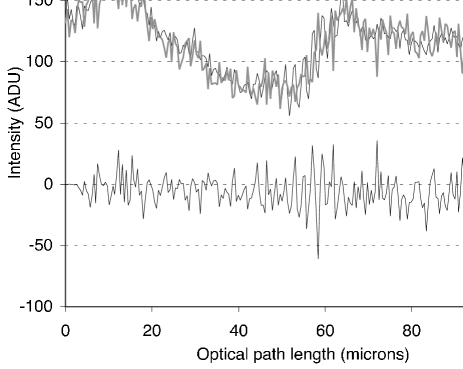
Figure 6: Photometric calibration of the $I_{1}$ signal. The raw $I_{1}$ signal is the black line in the upper part of the plot, the photometric calibration signal $\kappa_{1A}P_{A}-\kappa_{1B}P_{B}$ is the superimposed grey line, and the result of the subtraction is the lower curve.

5.2 Low pass filtering of photometric signals

The normalization by the $P$ signal is a critical step of the calibration. If $P$ presents too low values (“zero crossing”), the divisions of Eq. 5 and 6 will amplify the noise of the numerator. This is the reason why the $P_{A}$ and $P_{B}$ signals have to be filtered, to improve their SNRs. This is achieved using Wiener filters, that allow one to optimally filter the raw signal and to reject the detector noise. They are computed from the average power spectral density (PSD) of the photometric fluctuations of $P_{A}$ and $P_{B}$ using only the on-source spectra. We use the classical definition of the Wiener filter $W_{x}$ as computed from the signal $P_{x}$ and the noise $N_{x}$ (with $x=A$ or $B$, the Fourier transform being represented by the $\sim$ notation):

$$W_{x}=\frac{\widetilde{P_{x}}^{2}-\widetilde{N_{x}}^{2}}{\widetilde{P_{x}}^{2}}$$ (7)

As shown in Fig. 7 ($\theta$ Cen data), we estimate the PSD of the noise directly from the PSD of the signal by assuming that the photon shot noise and detector noise are constant with respect to frequency (white noise). The contribution from the photometric fluctuations is visible at low frequencies. Considering the high frequency part of the spectrum, we extrapolate the level of the PSD background to the lower frequencies. Due to the high SNR of the averaged PSD, the estimation of the background is precise enough to reconstruct $W_{A}$ and $W_{B}$. The first frequency for which the signal becomes smaller than the noise marks the practical limit of the Wiener filter, and the higher frequency values are set to zero. This method is more efficient than estimating the noise PSD from the off-source batch, as it directly takes into account the presence of photon shot noise, that also has to be removed. The resulting Wiener filters are presented in Fig. 8. The filtering of the photometric channels by these filters gives a clean $P$ signal, as shown in Fig. 9.

Figure 7: Average power spectral density of the $P_{A}$ and $P_{B}$ signals as measured on $\theta$ Cen. From top to botton: $\widetilde{P_{A}}^{2}$, noise model $\widetilde{N_{A}}^{2}$ (upper dotted line), $\widetilde{P_{B}}^{2}$, noise model $\widetilde{N_{B}}^{2}$ (lower dotted line).

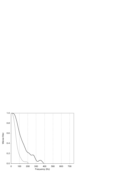
Figure 8: Wiener filters computed from $\theta$ Cen photometric signals (Fig. 7). $W_{A}$ is the upper line, and $W_{B}$ the lower line.

Figure 9: Photometric normalization signal $P$ (thick line), with the Wiener filtered $P_{A}$ (dashed line) and $P_{B}$ channels (thin line). $P$ is the geometric mean of the two filtered photometric channels.

5.3 Alternative normalization methods

If the SNR of the photometric channels $P_{A}$ and $P_{B}$ reaches too low values over the scan length, we choose to normalize the interferograms simply by averaging $P$ over the fringe length, instead of using the Wiener filtered signal. This allows us to significantly reduce the amplification of the noise due to the normalization division. The limit between the two regimes is usually set to 5 times the readout noise. For interferograms that present very low photometric signal over the fringe packet itself, we discard the scan as a significant bias can be expected on the modulated power. Both averaging and Wiener filtering are almost equivalent on the final calibrated interferograms, with a slight advantage to the Wiener filtering when the photometric fluctuations are important (as in the UT observations for example).

5.4 Interferogram subtraction

After their calibration, we subtract the two interferograms $I_{1\,cal}$ and $I_{2\,cal}$, in order to cancel the residual photometric fluctuations due to the uncertainty in the estimation of the $\kappa$ coefficients. This subtraction has proven to significantly enhance the immunity of the interferograms to the contamination coming from the photometric fluctuation background. Fig. 10 shows the calibrated and normalized interferometric signal $I_{1\,cal}$ and $I_{2\,cal}$, together with $I$ the result of the subtraction of these two signals defined as:

$$I=\frac{I_{1\,cal}-I_{2\,cal}}{2}$$ (8)

The combined signal $I$ is used for the integration of the fringe power to derive the visibility (Sect. 7). The advantage of using $I$ instead of using separately $I_{1\,cal}$ and $I_{2\,cal}$ for the integration of the fringe power is that all the correlated noise between the two signals is eliminated by the subtraction, while the fringes, perfectly opposed in phase, are amplified. This allows us to eliminate the residual photometric fluctuations as well as part of the noise introduced during the photometric calibration.

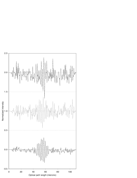
Figure 10: From top to bottom: $I_{1}$ normalized interferogram (black), $I_{2}$ normalized interferogram (grey), and the result $I$ of the subtraction of these two signals. For clarity, the $I_{1}$ and $I_{2}$ signals are shifted vertically by +2 and +1, respectively. The correlated noise has disappeared in the combined signal and the fringe packet appears more clearly.

6 Interferogram selection

6.1 Piston effect

The photometric calibration of the interferograms compensates for the incidence of wavefront corrugation across each subpupil of the interferometer, however it does not help remove the random phase walk (differential piston) between the two subapertures.

The differential piston, considered as a time-dependent OPD error $x(t)$, can be locally expressed by a polynomial development around a reference time $t_{0}$ (corresponding, for example, to the middle of the acquisition sequence):

$$x(t)=x_{0}+\dot{x}\ (t-t_{0})+\ddot{x}\ (t-t_{0})^{2}+...$$ (9)

The effect of the OPD perturbation on the interferogram, and its consequence on the coherence factor measurement, depends on the order:

• Zeroth order: the constant term $x_{0}$ can be seen as a global offset of the fringe packet. It is detected and corrected by the QL algorithm which centers the fringe packet in the middle of the interferogram.

• First order: The first order of the piston $\dot{x}$ changes the fringe velocity and induces a simple frequency shift in the PSD. It modifies the fringe peak position, but acts only as a homothetic compression or expansion of the fringe packet along the OPD direction. The first order piston has no immediate effect on the fringe visibility. However, if the shifting speed $\dot{x}$ of the fringe packet is too high, it can result in an undersampling of the fringes that will affect the visibility.

• Second and higher orders: Any term of order two (acceleration) and beyond breaks the linear relationship in the scan between time and OPD, and consequently the Fourier relationship which is at the basis of the visibility calculation, distorting the shape of the fringe peak. This introduces a non-linear, seeing induced multiplicative noise on the visibility measurements, which is the dominant noise source for strong signals (bright, unresolved objects).

Detailed studies of the properties of atmospheric piston can be found for example in Linfield et al. (linfield01 (2001)) and Di Folco et al. (difolco02 (2002)). When a dedicated fringe tracking instrument becomes available on the VLTI (e.g. FINITO, Gai et al. gai03 (2003)), most of the piston will be actively removed by a servo loop. It remains to be checked how the residuals will still limit the final visibility precision.

6.2 Quality control of the interferograms

The goal of the interferometric data processing is to extract the squared visibility $V^{2}$ of the fringes. The intermediate step to this end is to measure the squared coherence factor $\mu^{2}$ of the stellar light. This instrument dependent quantity characterizes the fraction of coherent light present in the total flux of the target. It is calibrated using observations of a known star, as described in Sect. 9. To avoid any bias on $\mu^{2}$, we have to reject the interferograms that do not contain fringes (false detections), or whose fringes are severely corrupted by the atmospheric turbulence (photometrically or by the piston effect). The selection procedure is in practice similar to a shape recognition process.

For this purpose, we measure in the wavelet power spectral density (WPSD) the properties of the fringe peak both in the time and frequency domains, and we subsequently compare them with the expected properties of a reference interferogram of visibility unity, derived from the spectral transmission of the instrument. In this paper, we will refer interchangeably to the “time domain” or “optical path difference (OPD) domain” for the WPSD, as they are linearly related through the scanning speed of the VINCI piezo mirror that is used to modulate the OPD. The fringe peak is first localized in frequency by the maximum of the WPSD, and then the full width at half maximum is computed along the two directions: time and frequency. As the fringe packet has been recentered before the calibration, its position in the time domain is zero. Three parameters are then checked for quality:

• peak width in the time domain (typically $\pm 50$% around the theoretical value is acceptable),

• peak position in the frequency domain ($\pm 30$%),

• peak width in the frequency domain ($\pm 40$%).

In principle, the variation of the fringe contrast over the spectral band should also be taken into account to create the theoretical reference interferogram. But in practice, as long as the visibility of the fringes does not cancel out for a wavelength located inside the spectral band of the observations, the shape of the interferogram remains very close to theoretical fringes of visibility unity. However, when the fringe visibility goes down to zero for a wavelength pertaining to the observation band, the fringe packet appears split in two parts in the time domain. Such a deviation from the “single packet” case can cause misidentifications, and eventually induce a bias on the derived $\mu^{2}$ value, as some valid interferograms would be rejected. In this case, one should use a dedicated broadband model to predict the reference interferogram, taking into account the expected angular size of the target. The selection criteria should then be adapted to match this reference (increased peak width, presence of two maxima in the WPSD,…). An alternative is to directly adapt the basis functions of the wavelet transform so that they match the predicted interferograms. We have not implemented these methods in our current processing algorithm, whose validity is thus limited to the cases when the visibility is above zero for all wavelengths in the observation band. If this condition is not realized, then the interferogram selection should be disabled, or at least the selection criteria should be made significantly less stringent, in particular regarding the fringe peak width.

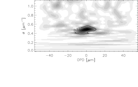
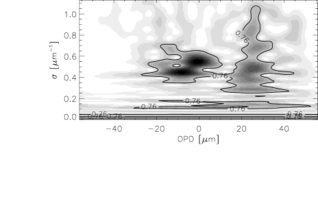
Figure 11: Wavelet power spectral densities of processed interferograms ($\sigma$ represents the wave number, i.e. the inverse of the wavelength). The upper figure shows the WPSD of a good quality interferogram: the energy is well confied in the fringe power peak. The bottom WPSD is affected by strong atmospheric piston: a significant part of the fringe power is spread outside of the theoretical fringe peak, both in time and frequency domains. The isocontours delimit 77 % and 76 % of the total modulated power, respectively.

Fig 11 shows two examples of interferogram WPSD, one of them being affected by atmospheric piston. The difference in terms of fringe peak shape is clearly noticeable, and leads to the rejection of the corrupted interferogram (bottom figure). This selection process has shown a very low false detection rate, and rejects efficiently the interferograms that are affected by a strong piston effect. However, limited piston of order two (and above) is not identified efficiently. The problem here is that the relevant properties for the estimation of the second order piston are currently difficult to measure with a sufficient SNR from the data, as they are masked by the order 1 piston. We expect that the introduction of the FINITO fringe tracker in 2004 will allow us to derive an efficient metric to reject the interferograms affected by a high order piston effect. After the fringe power integration (described in Sect. 7), we filter out the scans which $\mu^{2}$ deviates by more than 3 $\sigma$ from the median of the full batch of interferograms (usually 500 scans). This step prevents the presence of very strong outliers, which can appear due to the division introduced by the normalization of the interferograms (introduction of Cauchy statistics).

6.3 Immunity to selection biases

An essential aspect of the parameters used for the quality control of the fringe peak properties is that they are largely independent of the visibility of the fringes, and therefore do not create selection biases. In particular, the integral of the fringe peak (directly linked to the visibility) or its height are never considered in the selection. The parameters chosen in Sect. 6.2 clearly depend on the photometric SNR, but are independent of the visibility of the fringes, thanks to the calibration procedure described in Sect. 5.

The upper part of Fig. 12 demonstrates this independence in the difficult case of the batch of interferograms obtained on $\alpha$ Cen A. Despite the very low visibility of the fringes, no systematic deviation is visible for low photometric SNR values, as the dispersion is symmetric around the mean value. The same plot for $\theta$ Cen (Fig. 12 bottom) does not show any deviation either. A further discussion of the properties of the histogram of these measurements can be found in Sect. 8.3.

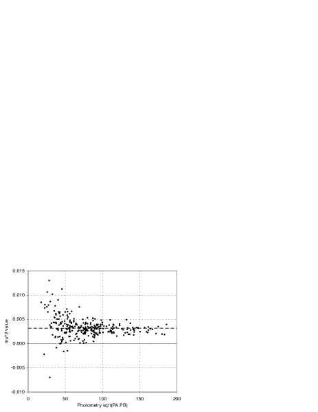
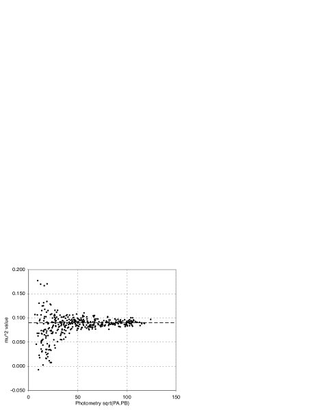
Figure 12: Squared coherence factor $\mu^{2}$ as a function of the photometric signal on the fringe packet, for the sample batches obtained on $\alpha$ Cen A (top) and $\theta$ Cen (bottom). The dashed lines show the mean value of the series derived using the bootstrap technique.

This means that the quality control described in this paragraph is not linked to the observable, and thus does not introduce a selection bias. Its effect in the case of the $\theta$ Cen and $\alpha$ Cen A observations is discussed in Sect. 8.3.

A critical case is when the visibility is extremely low. In this situation, the fringe peak will tend to blend in with the noise, which tends to make it appear broader and slightly displaced. Therefore, low-visibility data are more likely to be rejected than high-visibility data. This can introduce a bias towards higher $\mu^{2}$ for low-visibility observations: a scan with a +1 $\sigma$ deviation is accepted, but a scan with a -1 $\sigma$ deviation is more likely to be rejected as it fails the selection criteria. However, in this situation, the risk is high to fail to reject the spurious spikes that are created in the calibrated interferograms due to the division by the $P$ signal (Sect. 5). Without the selection procedure, the modulated power of these calibration artefacts will be integrated in the final $\mu^{2}$ value. As this power is essentially random, but always positive, these misidentifications would then result in a strong positive bias on the final $\mu^{2}$ value. For this reason, and in spite of the potential rejection of a small part of the valid interferograms, the application of the selection procedure results in a more reliable estimate of $\mu^{2}$, even for the very low visibility fringes. In any case, the careful examination of the statistical properties of the $mu^{2}$ histogram (see Sect. 8), and in particular of its skewness, allows us to detect a possible selection bias.

7 Visibility computation

7.1 Wavelet power spectral density

Once the interferogram has been calibrated and normalized, the squared coherence factor $\mu^{2}$ is measurable as the average modulated energy of the interference fringes over the batch. It is computed by integrating the power peak of the interferograms in the average WPSD (see also Appendix A and Sect. 7.2.1). The WPSD is a two dimensional matrix, examples of which are shown in Fig 11. For all wavelet transforms, we use the Morlet wavelet, which is defined as a plane wave multiplied by a Gaussian envelope. It closely matches the shape of the interferometric fringe packet. When computing a classical PSD, the interferogram is projected on a base of sine and cosine functions, which are not localized temporally. This means that the information of the position of the fringe packet is not used, and that the noise of the complete interferogram contributes to the measured power. On the other hand, the wavelet transformation projects the interferogram on a base of wavelets that are localized both in time and frequency, making full use of the localized nature of the modulated energy. As discussed in Appendix A, the modulated energy of the signal is conserved by the wavelet transform in the same way as through the classical Fourier transform.

7.2 Estimation of the squared coherence factor $\mu^{2}$

7.2.1 Fringe power integration

The average power spectral density of the $\alpha$ Cen A sample batch, computed using the wavelet transform, is shown in Fig. 13. To obtain this 1D spectrum from the original 2D WPSD matrices, we first project the WPSD matrix of each interferogram on the frequency axis, by integrating it over the fringe packet length (time axis). From this we obtain a series of one-dimensional vector PSDs, similar to the Fourier PSD but with a reduced noise. Before the averaging, we recenter each fringe peak using the frequency position information derived from the selection of the interferograms (Sect. 6). This step allows us to confine more tightly the energy of the peak, which is displaced by the first order piston effect. This reduces the influence of piston on the final $\mu^{2}$ value. The co-added 1D spectrum is the signal used for the final power integration to estimate the $\mu^{2}$ of the star.

The integration of the fringe power is typically done over 100 pixels in the time domain (20 fringes), and from 2 000 to 8 000 cm^-1 in the frequency domain (see also Sect. 8.1).

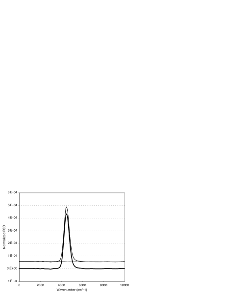
Figure 13: Average WPSD of the $\alpha$ Cen A observation. The original two-dimensional matrix has been integrated over the fringe packet length in the time domain. The resulting projection on the wave number axis allows one to visualize clearly the noise contribution. The subtracted noise model is shown by the dashed line. The final WPSD (thick line) shows no bias in spite of the large brightness of the star and very low squared coherence factor of the fringes ($\mu^{2}\approx 0.3$ %).

7.2.2 Removal of the WPSD background

The power in the fringe peak is contaminated by three additive components:

• the photon shot noise,

• the detector noise,

• the residual photometric fluctuations.

To estimate the modulated power of the fringes, it is essential to precisely remove these contributions from the PSD of the interferograms.

Perrin (perrin03a (2003)) has developed an analytical treatment of the photon shot noise based on its particular properties (Poisson statistics). The photon shot noise is perfectly white, as it is created from a purely random process. However, due to the calibration and normalization process of the interferograms, its translation onto the final interferometric signal $I$ could in theory deviate from this property and show a dependence with frequency. Such an effect has not been observed in practice on the VINCI data, and the uniform subtraction of the photon noise background from the PSD of the $I$ signal has proven to be very efficient. A good example of the ”whiteness” of the photon shot noise of the processed fringes can be found in Wittkowski et al. (wittkowski04 (2004)), where a very bright star ($m_{K}=-0.6$) was observed with the two 8 m telescopes UT1 and UT3 ($B=102.5$ m). In spite of the extremely large flux on the VINCI detector ($100$ m² collecting optics) and the very low visibility of the fringes ($V^{2}\simeq 10^{-2}$), the resulting PSD background is white, therefore validating our photon shot noise removal method under the most demanding conditions.

In order to fully justify our background removal procedure, we still have to verify the ”whiteness” of the detector noise, whose statistics and frequency structure depends on the type of detector and readout electronics used. The infrared camera of VINCI (LISA) is based on a HAWAII array, which is read using an IRACE controller (Meyer et al. irace (2000)). As only four pixels of the 1024x1024 array are actually used, an engineering grade detector was chosen for the instrument. It presents a large quantity of dead and hot pixels, and therefore it was necessary to thoroughly check its noise characteristics. This was achieved during extensive laboratory testing, and is also verified automatically for each observation. It appeared that the LISA detector noise is perfectly white, without any significant electronic interference signature.

This satisfactory behavior of the detector and photon shot noises allows us to remove them simultaneously by subtracting to the $\mu^{2}$ value of each interferogram an average of its WPSD at high frequency, measured outside of the domain of frequency of the interferometric fringes. To correct for potential residuals pf the photometric calibration, we fit a linear model of the residual background to the average WPSD of the interferograms in the batch. In this procedure, we allow for a limited slope of the background model, in order to correct a possible residual power from photometry. Thanks to the averaging of a large number of scans, the noise on the average WPSD low, and the fitting procedure is very precise. Most of the time, and even for the most important fluctuation cases (Unit Telescopes in multispeckle mode), the contribution of the residual photometric noise is totally negligible on the combined interferogram $I$ obtained from the subtraction of the calibrated signals $I_{1\,cal}$ and $I_{2\,cal}$ (Eq. 8).

An illustration of the background quality is presented in Fig. 13. The WPSD background noise appears perfectly white, even at the very enlarged scale used to visualize the very small fringe peak of $\alpha$ Cen A ($\mu^{2}\approx 0.3$ %). In particular, no “color” or electronic interference (“pickup”) are present. The model of the removed noise is also plotted on the two figures, showing that the subtraction is very clean.

7.3 Estimation of the statistical error

To compute the statistical error on the $\mu^{2}$ estimation, we integrate separately the fringe power in each WPSD of the batch, correct the detector and photon shot noise biases individually, and use a weighted bootstrapping technique on this set of measurements. Our sample is made of $N$ pairs $(\mu^{2}_{i},w_{i})$ where $\mu^{2}_{i}$ is the squared coherence factor obtained by integrating the WPSD of the scan of rank $i$ in the series and $w_{i}$ is its associated weight. It is defined as the average level of the photometric signal $P$ over the fringe packet length (20 fringes in the $K$ band) multiplied by the inbalance between the two photometric channels $P_{A}$ and $P_{B}$:

$$w_{i}=\frac{\min(\overline{P_{A,i}},\overline{P_{B,i}})}{\max(\overline{P_{A,i}},\overline{P_{B,i}})}\ \overline{\left(\sqrt{P_{A,i}P_{B,i}}\right)}_{\rm Fringes}$$ (10)

It characterizes well the clarity of the total photometric signal that contributes to the formation of the fringes. The final dispersion of the $\mu^{2}$ values is reduced by this weighting. The detailed description of the weighted bootstrapping method used for the computation of the error bars is given in Appendix B.

The bootstrapping technique has the important advantage of not making any assumption on the type of statistical distribution that the data points follow. In particular, it is more reliable than the classical approach that assumes a Gaussian distribution of the measurements. Skewness and other deviations from a Gaussian distribution are automatically included in the error bars, which can be asymmetric.

The statistical dispersion of VINCI measurements shows two regimes: for bright stars the precision is limited by the piston and photon shot noise, while for the fainter objects, the main contributor to the dispersion is the detector noise of the camera, and the precision degrades rapidly. A discussion of the different types of noise intervening in the visibility measurements can be found for instance in Colavita (colavita99 (1999)) and Perrin (perrin03a (2003)). The $\mu^{2}$ measurements discussed in this paper have a relative statistical precision of $\pm 3.00$% for $\alpha$ Cen A, and $\pm 0.53$% for $\theta$ Cen. The lowest relative statistical dispersion $\sigma(\mu)/\mu$ reached up to now on the coherence factor with VINCI is in the 2% range. Under good conditions, this translates into a bootstrapped statistical error of less than $\pm 0.1\%$ on $\mu$ for 5 minutes of observations.

8 Post-processing quality control

After a batch of interferograms is processed, several quality controls are performed in order to detect any problem in the resulting visibility values and statistical error bars. This step is essential to ascertain the quality of the interferometric data, as it can vary depending on the atmospheric conditions (e.g. seeing, coherence time) and on the general behavior of the instrument (e.g. injection of the stellar light in the optical fibers, beam combiner properties, polarization mismatch of the two beams).

8.1 Power peak integration boundaries

A potentially damaging effect of the atmospheric piston on the visibility of the fringes is that it tends to move the position of the fringe peak, and to spread it over a wider frequency range. If the frequency boundaries for the integration of the fringe peak are set too tight, the result could be that part of the modulated power is not taken into account, creating a bias. These boundaries are automatically changed as a function of the ground baseline length to account for the increased piston strength on longer baselines. They are not modified as a function of the projected baseline, and are thus identical for scientific targets and calibrators.

To check for the presence of such an effect, we measure the fringe peak shape in the WPSD. More precisely, we estimate its central wave number, full width at half maximum, as well as the limit wave numbers for which the background level is reached. Using these extended limits, we integrate the fringe power and compare this value to the one obtained with the user-specified wave number limits. If a discrepancy is found at a significant level, the batch is considered dubious and can be rejected after further examination.

8.2 Histogram properties

As the noise sources acting on the $\mu^{2}$ values have normal statistics, it is expected that the distribution of the $\mu^{2}$ values over the batch is also normal. Although the bootstrapping procedure used to compute the $\mu^{2}$ error bars is not sensitive to the type of distribution, a large skewness or kurtosis would betray a problem in the calibration of the interferograms that could eventually bias the final $\mu^{2}$ value. The relevant parameters for this verification are the skewness coefficient $s$ (third moment of the distribution) defined as:

$$s=\sum_{i=1}^{N}{\frac{(\mu^{2}_{i}-\overline{\mu^{2}})^{3}}{(N-1)\sigma^{3}}}\\$$ (11)

and the kurtosis coefficient $k$ (fourth moment):

$$k=\sum_{i=1}^{N}{\frac{(\mu^{2}_{i}-\overline{\mu^{2}})^{4}}{(N-1)\sigma^{4}}}-3$$ (12)

where $\mu^{2}_{i}$ are the squared coherence factor values, $\sigma$ the standard deviation, $\overline{\mu^{2}}$ the unweighted average, and $N$ the number of scans. The skewness characterizes the presence of a ”tail” on the histogram. A large value of $s$ is therefore a symptom of a potential bias problem in the distribution, as a significant number of values are either too large or too small compared to the average value of the sample. A positive kurtosis coefficient means a distribution more peaked than the normal one. However, it should be stressed that the kurtosis is not a very robust parameter to assess if the sample is drawn from a normal distribution. It requires a large number of sample values to be relevant, and it is very sensitive to the presence of outliers. Therefore, it should only be used in conjunction with other statistical tests. A range of $\pm 0.5$ can be considered acceptable for $k$. When random samples are drawn from a normal population, the resulting skewness coefficients will fall into the range $\pm 0.18$, with a probability of 90%. We therefore choose this value as an acceptable range.

8.3 Application to $\theta$ Cen and $\alpha$ Cen A

Table 4 gives the reasons for the rejection of the interferograms of the $\theta$ Cen and $\alpha$ Cen A batches. In the case of $\alpha$ Cen A, a larger number of interferograms are rejected due to the very low visibility of the fringes.

Table 4: Reasons for the rejection of $\theta$ Cen and $\alpha$ Cen A interferograms during the processing. The lower part of this table corresponds to the selection criteria related to the atmospheric piston effect.

Reason	$\theta$ Cen	$\alpha$ Cen A
Photometry too low	77	24
Large OPD jump	13	47
Fringes at edge	6	27
Fringe packet width	1	47
Fringe peak position	3	40
Fringe peak width	5	33
Outliers (3 $\sigma$)	9	5
Total number of rejected scans	114/500	223/500

The measured statistical properties of the processed interferograms of $\theta$ Cen and $\alpha$ Cen A are given in Table 5. The values in brackets were obtained by disabling the piston selection of the interferograms (based on the fringe packet width, and on the position and width of the fringe peak in the power spectrum of the interferogram). The comparison of the selected vs. non-selected versions of the data processing shows that the piston selection has a positive effect on the dispersion of the measurements. For $\theta$ Cen, the difference is minimal between the two kinds of processing. In particular, the total number of processed interferograms is almost identical for the two cases. However, for $\alpha$ Cen A, the difference is clearly noticeable, as the final error bars are 60% larger when the selection is disabled, in spite of a total number of processed scans approximately 40% larger. The skewness of the histogram is also much larger in this case (by a factor of 20). This clearly shows the advantage of the fringe selection procedure, in particular for the rejection of the calibration artefacts (false detections) in the very low visibility case (see also Sect. 6.3).

Table 5: Statistical properties of the $\theta$ Cen and $\alpha$ Cen A sample batches. The values obtained when disabling the selection of the interferograms based on their piston properties are given in brackets for comparison.

	$\theta$ Cen	$\alpha$ Cen A
Reduced scans	386 (395)	277 (391)
Average $\mu^{2}$ (%)	8.995 (8.999)	0.3180 (0.2949)
Stat. error ($1\sigma$)	0.048 (0.050)	0.0095 (0.0142)
Rel. error $\sigma/\mu^{2}$	0.53% (0.56%)	3.00% (4.81%)
Skewness $s$	$+0.023$ ($+0.013$)	$-0.007$ ($+0.160$)
Kurtosis $k$	$+0.164$ ($+0.062$)	$+0.044$ ($-0.042$)

In the case of $\theta$ Cen (Fig. 14) and $\alpha$ Cen A (Fig. 15), no skewness is present. For $\theta$ Cen, a small positive kurtosis $k\approx 0.16$ is detected, meaning that the distribution is slightly too peaked (leptokurtic, as opposed to a platykurtic distribution that is too flat). However, it is easily inside the acceptable range ($\pm 0.5$), and this property is taken into account in the bootstrapped error bars.

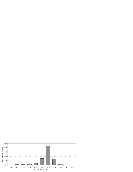
Figure 14: Histogram of the $\mu^{2}$ values obtained on $\theta$ Cen. No significant skewness is present.

Figure 15: Histogram of the $\mu^{2}$ values obtained on $\alpha$ Cen A. A moderate skewness is present towards higher $\mu^{2}$ values.

9 Visibility calibration

9.1 Principle

The data reduction software of VINCI yields accurate estimates of the squared modulus of the coherence factor $\mu^{2}$, which is linked to the squared object visibility $V^{2}$ by the relation:

$$V^{2}=\frac{\mu^{2}}{T^{2}}$$ (13)

where $T^{2}$ is the response of the system to a point source, also called transfer function (hereafter TF), interferometric efficiency, or system visibility. It is measured by bracketing the science target with observations of calibrator stars whose $V^{2}$ is supposed to be known a priori. The accuracy of our knowledge of the calibrator angular diameter, and the precision with which we estimate its $\mu^{2}$ are therefore decisive for the final quality of the scientific target observation. Typically, the scientific targets are bracketed by calibrator observations, so as to be able to verify the stability of the TF. In this respect, the VLTI has often proved to be stable at a scale of a few percent over several nights. Nevertheless, and to guarantee the quality of the VINCI data, calibrators are regularly observed during the night, before and after each scientific target.

9.2 Interferometric transfer function estimation

9.2.1 Transfer function model

By nature, the interferometric TF is affected by a large number of parameters: atmospheric conditions (seeing, coherence time), polarization (incidence of the stellar beams on the siderostat mirrors, spectrum of the target, etc…). These effects combine to make $T^{2}$ a stochastic variable, that can evolve over a wide range of timescales. In order to estimate its value and uncertainty on a particular date at which it was not directly measured (e.g. during the observation of a scientific target), it is necessary to use a model of its evolution. Such a model relies necessarily on an hypothesis, for instance that the value of $T^{2}$ is constant between two (or more) calibrator observations, that it varies linearily, quadratically, or any higher order model. Let us now evaluate the most suitable type of TF model for the observations with VINCI.

As a practical example, Fig. 16 shows the evolution of $T^{2}$ over one night of observations, with a typical sampling rate of one measurement every 15 minutes. This series of 27 observations was obtained during the night of 29 May 2003 on the E0-G0 baseline (16 m ground length). A number of different stars with known angular diameters were observed, covering spectral types in the G-K range. During these observations, spread over 8 hours, the seeing evolved from 1.0 to 2.0 arcsec, the altitude of the observed objects was distributed almost uniformly between 25 and 80 degrees, and the azimuth values covered 15 to 90 degrees (N = 0, E = 90). Due to this broad range of conditions, this series represents a worst case in terms of TF stability. As a reminder, under normal conditions, a calibrator is selected as close as possible to the scientific target, in time, position and spectral type.

Over the whole night, the overall stability is satisfactory, with a dispersion of $\sigma_{\rm tot}=0.64$% around the average value of $\overline{T^{2}}=41.75$%. In order to estimate the external dispersion $\sigma_{\rm ext}$ of the transfer function over the night (due to the atmosphere and instrumental drifts), we can subtract the average of the intrinsic variances $\sigma_{i}^{2}$ of the $T_{i}^{2}$ values $\sigma_{\rm int}^{2}$ from the total variance $\sigma_{\rm tot}^{2}$:

$$\sigma_{\rm ext}^{2}=\sigma_{\rm tot}^{2}-\sigma_{\rm int}^{2}.$$ (14)

The average precision of each individual $T^{2}$ measurement in our sample night is $\sigma_{\rm int}=0.21\%$. This gives an external dispersion of $\sigma_{\rm ext}=0.60\%$. In this particular case, the external dispersion is thus dominant over the internal measurement errors, by a factor of almost three.

From this example, we can conclude that the rate of one measurement every 15 minutes is insufficient to sample the fluctuations of the TF. Due to this, we do not gain in precision by interpolating the TF values using a high order model (quadratic, splines,…). In the current state of the VLTI (siderostat observations), the most adequate model for the estimation of the TF is thus a constant value between the observations of the calibrators. The 1.8 m Auxiliary Telescopes will soon allow us to sample the TF with a much higher rate, of the order of 1 minute, and higher order models of the TF variations could become necessary. As we are dominated by the external dispersion $\sigma_{\rm ext}$, the uncertainty on the TF has to be estimated from the dispersion of the individual $T^{2}$ measurements obtained before and after the scientific target, without averaging of their associated error bars.

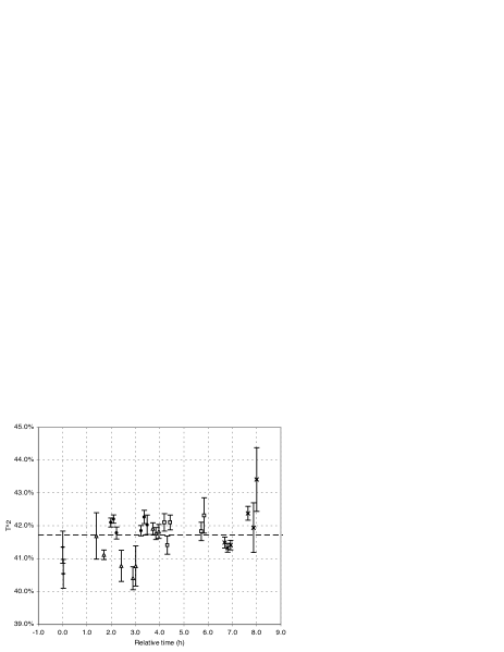
Figure 16: Evolution of the transfer function $T^{2}$ during one night (2002-05-29) on the E0-G0 baseline of the VLTI (16 m in ground length). Each symbol corresponds to a different star.

9.2.2 Refinement of the transfer function model

Under good and stable conditions, the random dispersion of $T^{2}$ introduced by the atmosphere can be very low between two consecutive observations of a calibrator. In this case, we want to evaluate the true uncertainty on the model $T^{2}$ by comparing the hypothesis of stability to the calibrator observations, and subsequently refine the hypothesis used to estimate the error bar on $T^{2}$.

The observational strategy chosen with VINCI is to record several series of interferograms consecutively for each calibrator observation (typically three), over a period of about 15 minutes. To decide if the atmospheric and instrumental conditions are stable over this period, we compute the following $\chi^{2}$ expression:

$$\chi^{2}_{\rm tot}=\sum_{i}\frac{(T_{i}^{2}-\overline{T^{2}})^{2}}{\sigma_{{\rm stat},i}^{2}}$$ (15)

where $T_{i}^{2}$ are the consecutive estimates of the TF obtained on the calibrator, $\sigma_{{\rm stat},i}^{2}$ the statistical error of each measurement, and $T^{2}$ the weighted average of the $T_{i}^{2}$ values (using the inverse of the statistical variance as weights). If the resulting $\chi^{2}$ is small (less than 3), then the hypothesis that the TF is constant is probably true: the $T_{i}^{2}$ values can be averaged and the global statistical error bar reduced accordingly. If not, then this hypothesis cannot be made, and a realistic approach is to consider as the true measurement error of the average TF the standard deviation of the $T_{i}^{2}$ sample.

When several series of interferograms are obtained on the same calibrator and the conditions described above are verified, the resulting estimates of the TF can be averaged in order to reduce the attached statistical error bar. However, the systematic error introduced by the a priori uncertainty on the angular size of one calibrator cannot be reduced by repeatedly observing this star, but only by combining the TF measurements obtained on independent objects.

9.3 Application to the sample observation of $\alpha$ Cen A

In the case of the observations described in this paper, $\theta$ Cen was observed one hour before $\alpha$ Cen A. Assuming a UD angular diameter of $\theta_{\rm UD}=5.305\pm 0.020$ mas (Kervella et al. 2003b ), and taking into account the spectrum of the source and the bandwidth averaging effect (also called bandwidth smearing, see e.g. Davis et al. davis00 (2000)), we expect a squared visibility of $V_{\rm theo}^{2}=0.1796$ and a $1\,\sigma$ systematic uncertainty $\sigma_{\rm syst}=\pm 0.0027$ for the 65.929 m projected baseline (weighted average over the interferogram series). As we observed an instrumental coherence factor of $\mu^{2}=0.08995\pm 0.00048$, the transfer function $T^{2}$ is estimated to be:

$$T^{2}=\frac{0.08995\ [\pm 0.00048]_{\rm stat}}{0.1796\ [\pm 0.0027]_{\rm syst}}.$$ (16)

Using the relations detailed in Appendix C to compute the error bars of the ratio $\mu^{2}/T^{2}$, we obtain

$$T^{2}=0.5010\ [\pm 0.0027]_{\rm stat}\ [\pm 0.0077]_{\rm syst}.$$ (17)

As we consider here only one calibrator observation, we cannot estimate the external dispersion of $T^{2}$, and we consider only the internal statistical and systematic error bars. As a remark, this $T^{2}$ value is not identical to the one computed in Sect. 9.2.1, as it was obtained more than one month later. The VINCI coupler is known to be sensitive to long term temperature variations (over a timescale of weeks), an effect that can explain the observed difference.

The squared visibility value of $\alpha$ Cen A is then:

$$V_{\rm\alpha\,Cen}^{2}=0.00635\ [\pm 0.00019]_{\rm stat}\ [\pm 0.00010]_{\rm syst}.$$ (18)

The uncertainty on this value is dominated by the statistical error, despite the importance of the systematic error on the value of $T^{2}$. The average baseline of this measurement is 61.470 m, and we can now deduce the uniform disk model angular diameter of $\alpha$ Cen A, $\theta_{\rm UD}=8.305\pm 0.024$ mas, which is very close to the published value of $\theta_{\rm UD}=8.314\pm 0.016$ mas from Kervella et al. (2003b ). This computation takes into account the wavelength averaging effect due to the broadband $K$ filter of VINCI as described by Kervella et al. (2003b ).

10 Conclusion

We have described the data reduction methods that are used on VINCI, the VLTI Commissioning Instrument. In particular, we detailed the photometric calibration of the interferometric signals, followed by the normalization of the fringes, and the subtraction of the two calibrated interferograms. Due to the efficient spatial filtering provided by the single-mode optical fibers, this procedure provides a clean calibration of the fringes, and allows us to derive the squared coherence factor $\mu^{2}$ with high accuracy. Combined with observations from a calibrator star, it yields the squared visibility $V^{2}$. This value can be interpreted physically through the use of a dedicated model of the observed object. Applying the data reduction methods described in this paper to sample data from $\alpha$ Cen A yields a realistic value of its uniform disk angular diameter. Our procedures can easily be adapted to other single mode interferometric instruments. In particular, they can be generalized to spectrally dispersed fringes and to a multiple beam recombiner using the integrated optics technology (Kern et al. kern03 (2003)). Such a device could allow the simultaneous recombination of the beams from the four 8 m Unit Telescopes and four Auxiliary Telescope of the VLTI in a compact instrument.

Appendix A The wavelet transform

The wavelet transform belongs to the class of time-frequency transforms which are powerful tools to study non-stationary processes such as turbulent flows in fluid mechanics. Wide band coaxial interferograms recorded through a turbulent atmosphere can be strongly distorted due to the differential piston effect and fast photometric fluctuations. In this context, the wavelet transform is an efficient tool to study and analyse the interferograms recorded from the ground.

The continuous wavelet transform (hereafter CWT) is defined by:

$$W\left(s,\tau\right)=\frac{1}{\sqrt{s}}\int_{-\infty}^{+\infty}f\left(t\right)\psi^{*}\left(\frac{t-\tau}{s}\right)\,dt$$ (19)

where $f(t)$ is the signal defined as a function of time, $\psi\left(t\right)$ the chosen wavelet function, $\psi^{*}$ its complex conjugate, $s$ the scale, and $\tau$ the translation.

For the present application of the CWT to interferometry, we have chosen to use the Morlet wavelet, that is defined as a Gaussian envelope multiplied by a plane wave (Goupillaud et al. goupillaud84 (1984); Farge farge92 (1992)):

$$\psi\left(\eta\right)=\exp{(i2\pi\nu_{0}\eta)}\ \exp{(-\eta^{2}/2)}$$ (20)

where $\eta$ is the non dimensional time parameter and $\nu_{0}$ is the non dimensional frequency. Initially used for the analysis of seismic signals, the Morlet wavelet is a good approximation of the fringe pattern produced by VINCI. The data processing methods presented here make extensive use of this particular wavelet for the recognition and localization of the fringes (Sect. 4.2) and subsequently for the integration of the modulated power of the interference fringes (Sect. 7). Fig 17 shows the shape of the imaginary part of the Morlet wavelet assuming typical parameters for the processing of data from the MONA beam combiner ($K$ band).

If we now express the CWT in the Fourier domain (Eq. 21), it appears clearly that the CWT is a filtered version of the signal for different sets of filters:

$$W(s,\tau)=\sqrt{s}\int_{-\infty}^{+\infty}\widehat{f}\left(\nu\right)\widehat{\psi}^{*}\left(s\nu\right)e^{i\,2\pi\nu\tau}\,d\nu$$ (21)

Since the CWT is simply a convolution between the signal $f\left(t\right)$ and expanded/contracted versions of the wavelet function (Eq. 19), the Morlet wavelet is very efficient to analyse wide-band coxial interferograms. The CWT of an interferogram using the Morlet wavelet is a complex quantity and its maximum energy is found for the wavelet that is most similar to the recorded interferogram.

The CWT using the Morlet wavelet is not orthogonal but since it relies on a set of filtered versions of the signal with strong redundancy, the original signal can easily be reconstructed (Farge farge92 (1992); Perrier perrier95 (1995)). The energy properties of Wavelets are similar to the ones of the Fourier analysis, with the equivalent of the Parseval theorem (Perrier perrier95 (1995)). We have therefore the equivalence of the two following expressions of the energy $E$ of the signal:

$$E=\frac{1}{2\,C_{\psi}}\int_{0}^{+\infty}\int_{-\infty}^{+\infty}\left|W(s,\tau)\right|^{2}\,\frac{ds}{s^{2}}\,\,d\tau$$ (22)

$$E=\int_{-\infty}^{+\infty}\left|\widehat{f}\left(\nu\right)\right|^{2}\,d\nu$$ (23)

with the coefficient $C_{\psi}$ defined as:

$$C_{\psi}=\int_{-\infty}^{+\infty}\frac{\left|\psi\left(s\,\nu\right)\right|^{2}}{\nu}\,d\nu$$ (24)

As a consequence, we are able to recover the modulated energy of the original signal (the interferometric fringes) by integrating its wavelet power spectrum over the time and frequency regions where the interferogram is present.

Compared to the classical Fourier analysis, such an approach allows to minimize the biases due to both the white and colored (frequency dependent) noises. Thanks to its localization both in time and frequency, the Morlet wavelet is better suited to the study of interferometric fringe packets than the classical Fourier base functions (sine and cosine), as the noise present outside of the fringe packet in the scan is excluded from the integrated power. The interested reader will find a more detailed treatment of the wavelet transform in Daubechies (daubechies92 (1992)), Farge (farge92 (1992)),Perrier (perrier95 (1995)) and Mallat (mallat99 (1999)).

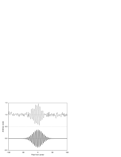
Figure 17: VINCI interferometric fringes (upper curve, from a processed interferogram of $\theta$ Cen) and the Morlet wavelet function imaginary part (bottom curve).

Appendix B Computation of weighted bootstrapped error bars

Originally developed by Efron (efron79 (1979)), the bootstrap analysis, also called sampling with replacement, consists of constructing a hypothetical, large population derived from the original measurements and estimate the statistical properties from this population. This technique allows us to recover the original distribution characteristics without any assumption on the properties of the underlying population (e.g. Gaussianity). An introduction to bootstrap analysis can be found in Efron (efron93 (1993)) and Babu (babu96 (1996)).

Our implementation of the bootstrapping technique draws, with repetition, a large number $M$ of samples containing $N$ elements from the original set of measurements $(\mu^{2}_{i},w_{i})$, also $N$ elements in length. $\mu^{2}_{i}$ designates the squared coherence factor associated with the scan of rank $i$ in the series, and $w_{i}$ is its associated weight. The result of this drawing is an $N\times M$ matrix of $(\mu^{2}_{k,j},w_{k,j})$ pairs ($1\leq k\leq N$; $1\leq j\leq M$). The fact that the same element of the original data set can be repeated several times in the drawing is essential, as it allows us to create independent samples. Typically, several thousand samples are obtained from the original data, which contains a few hundred $\mu^{2}$ values. The weighted average values $\mu^{2}_{k}$ are computed for each of the $N$ drawings:

$$\mu_{j}^{2}=\frac{1}{\left(\sum_{k=1}^{N}w_{k,j}\right)}\sum_{k=1}^{N}w_{k,j}\mu_{k,j}^{2}$$ (25)

The resulting ensemble $[\mu^{2}_{j}]$ ($M$ elements) is sorted in ascending order, and reindexed with the percentiles of the rank of each value in the set:

$$\mu^{2}_{0/M},...,\mu^{2}_{j/M},...,\mu^{2}_{M/M}$$ (26)

The 16 % lower and upper values are discarded, and the new extremes values of this vector give the limits of the 68 % confidence interval:

$$\mu^{2}_{\rm min}=\mu^{2}_{\ 0.16}\ ;\ \ \ \mu^{2}_{\rm max}=\mu^{2}_{\ 0.84}$$ (27)

This is the probabilistic definition of 1 $\sigma$ error bars, and we therefore obtain the $\sigma_{+}$ and $\sigma_{-}$ asymmetric error bars through:

$$\sigma_{+}=\mu^{2}_{\rm max}-\overline{\mu^{2}}\ ;\ \ \ \ \sigma_{-}=\overline{\mu^{2}}-\mu^{2}_{\rm min}$$ (28)

where $\overline{\mu^{2}}$ is the weighted average of the original sample $[\mu^{2}_{i}]$ using the weights $[w_{i}]$. The same process can be applied using 2.5–97.5 % percentile limits to obtain the error bars equivalent to $2\,\sigma$, and 0.5–99.5 % for $3\,\sigma$.

Alternatively, one can derive the bootstrapped variance $\sigma_{\rm BS}^{2}$ directly from the $\mu^{2}_{k}$ ensemble:

$$\sigma^{2}_{\rm BS}=\frac{1}{M}\sum_{j=1}^{M}\left(\mu^{2}_{j}-\overline{\mu^{2}}\right)^{2}$$ (29)

The internal bias $b_{\rm BS}$ of the population is given by:

$$b_{\rm BS}=\overline{\mu_{j}^{2}}-\overline{\mu^{2}}$$ (30)

This bias is naturally taken into account in the computation of the confidence interval limits as described above.

Appendix C Statistical and systematic errors of the ratio of $\mu^{2}$ and $T^{2}$

In the expression of $T^{2}$ of Eq. 16, we have to separate the contributions from the systematic uncertainty on the calibrator knowledge, and the statistical error of the instrumental measurement of $\mu^{2}$. While these two terms contribute to the global uncertainty on the squared visibility $V^{2}$, their nature is fundamentally different. While it is possible to reduce the statistical error by averaging several measurements, the systematic uncertainty originating in the calibrator diameter error bar will not be changed. This last term is therefore a fundamental limitation to the absolute precision of the visibility measurement. This limit can be reduced by using several calibrators, or by selecting very small stars as calibrators. We then benefit from the fact that the visibility function $V^{2}(B,\theta)$ for a stellar disk is nearly flat when the star is not significantly resolved, and the resulting systematic error on $V^{2}$ remains small.

Considering a symmetric error bar on the assumed angular diameter of the calibrator, the resulting error bar on the $V^{2}$ estimate is in general not exactly symmetric, due to the non linearity of the visibility function. In practice, asymmetric error bars are easily manageable numerically. However, in order to simplify the notations in the present discussion, we make the assumption that this asymmetry is negligible.

The estimation of the two kinds of error contributions relies on an approximation of the Cauchy statistical law characteristics. When dividing two normal statistical variables $x$ and $y$ of respective means and standard deviations $(\overline{x},\sigma_{x}^{2})$ and $(\overline{y},\sigma_{y}^{2})$, the resulting ratio $x/y$ follows a Cauchy statistics that has, strictly speaking, no defined mean value. It is therefore necessary to make an approximation for the case when $\sigma_{y}\ll\overline{y}$. In this case, a second order approximation of the mean $\overline{z}$ and variance $\sigma^{2}_{z}$ of $z=x/y$ is given by Browne (browne02 (2002)):

$$\overline{z}=\frac{\overline{x}}{\overline{y}}\left(1+\frac{\sigma_{y}^{2}}{\overline{y}^{2}}\right)$$ (31)

$$\sigma_{z}^{2}=\frac{\overline{x}^{2}}{\overline{y}^{2}}\left(\frac{\sigma_{x}^{2}}{\overline{x^{2}}}+\frac{\sigma_{y}^{2}}{\overline{y}^{2}}-\frac{\sigma_{y}^{4}}{\overline{y}^{4}}\right)$$ (32)

It is not possible to obtain a meaningful average value of the ratio $x/y$ if the standard deviation $\sigma_{y}$ of the denominator $y$ is not small compared to its average value. As a remark, the average value of $x/y$ is in general different from $\overline{x}/\overline{y}$.

The average value of the transfer function $T^{2}$ and its associated statistical error bars are computed by replacing in formulas 31 and 32 the values of $(\overline{x},\sigma_{x}^{2})$ and $(\overline{y},\sigma_{y}^{2})$ by the following terms:

$$\overline{x}\rightarrow\left[\mu^{2}\right]_{\rm\theta\,Cen}\ \ \ \ \ \ \ \ \ \ \ \ \ \ \ \sigma_{x}^{2}\rightarrow\left[\sigma_{\rm stat}\right]_{\theta\,Cen}^{2}$$ (33)

$$\overline{y}\rightarrow\left[V^{2}_{\rm theo}\right]_{\theta\,Cen}^{2}\ \ \ \ \ \ \ \ \ \ \ \sigma_{y}^{2}\rightarrow 0$$ (34)

Similarly, the systematic error is computed using the replacements:

$$\overline{x}\rightarrow\left[\mu^{2}\right]_{\rm\theta\,Cen}\ \ \ \ \ \ \ \ \ \ \ \ \ \ \ \sigma_{x}^{2}\rightarrow 0$$ (35)

$$\overline{y}\rightarrow\left[V^{2}_{\rm theo}\right]_{\theta\,Cen}^{2}\ \ \ \ \ \ \ \ \ \ \ \sigma_{y}^{2}\rightarrow\left[\sigma_{\rm theo}\right]_{\theta\,Cen}^{2}$$ (36)

Applying this computation to the numerical values found for $\theta$ Cen, we find:

$$T^{2}=0.5009\ [\pm 0.0027]_{\rm stat}\ [\pm 0.0077]_{\rm syst}$$ (37)

The uncertainty on this value is dominated by the systematic error. The only remaining calibration step is now to divide the $\mu^{2}$ value obtained on $\alpha$ Cen A by the $T^{2}$ value. Again, we have to separate the two contributions on the error by replacing in the above formulas the mean values and standard deviations of $x$ and $y$ by the following terms for the statistical error:

$$\overline{x}\rightarrow\left[\mu^{2}\right]_{\rm\alpha\,Cen}\ \ \ \ \ \ \ \ \ \ \ \ \ \ \ \sigma_{x}^{2}\rightarrow\left[\sigma_{\rm stat}\right]_{\alpha\,Cen}^{2}$$ (38)

$$\overline{y}\rightarrow T^{2}\ \ \ \ \ \ \ \ \ \ \ \ \ \ \ \ \ \ \ \ \ \ \ \ \sigma_{y}^{2}\rightarrow\left[\sigma_{\rm stat}\right]^{2}_{T^{2}}$$ (39)

while the systematic error is computed using

$$\overline{x}\rightarrow\left[\mu^{2}\right]_{\rm\alpha\,Cen}\ \ \ \ \ \ \ \ \ \ \ \ \ \ \ \sigma_{x}^{2}\rightarrow 0$$ (40)

$$\overline{y}\rightarrow T^{2}\ \ \ \ \ \ \ \ \ \ \ \ \ \ \ \ \ \ \ \ \ \ \ \ \sigma_{y}^{2}\rightarrow\left[\sigma_{\rm syst}\right]^{2}_{T^{2}}$$ (41)

We obtain the calibrated squared visibility of $\alpha$ Cen A:

$$V_{\rm\alpha\,Cen}^{2}=0.00635\ [\pm 0.00033]_{\rm stat}\ [\pm 0.00010]_{\rm syst}$$ (42)

- (1) Babu, G. J. & Feigelson, E. D. 1996, Astrostatistics, Chapman & Hall, London
- (2) Berger, J.-P., Haguenauer, P., Kern, P., et al. 2001, A&A, 376, 31
- (3) Bordé, P., Coudé du Foresto, V., Chagnon, G. & Perrin, G. 2002, A&A, 393, 183
- (4) Browne, J. M. 2002, Probabilistic Design Course Notes, available at http://www.ses.swin.edu.au/homes/browne
- (5) Cayrel de Strobel G., Soubiran C., Ralite N. 2001, A&A, 373, 159
- (6) Cohen, M., Walker, R. G., Carter, B. et al. 1999, AJ, 117, 1864
- (7) Colavita, M. M. 1999, PASP, 111, 111
- (8) Coudé du Foresto, V., Ridgway, S., Mariotti, J.-M. 1997, A&A Suppl. Series, 121, 379
- (9) Coudé du Foresto, V., Perrin, G., Ruilier, C., et al. 1998, Proc. SPIE 3350, 856
- (10) Daubechies, I. 1992, Ten lectures on wavelets, Proc. CBMS-NSF conf., June 1990, in Philadelphia: Society for Industrial and Applied Mathematics, 1992
- (11) Davis, J., Tango, W. J. & Booth, A. J. 2000, MNRAS, 318, 387
- (12) Derie, F. 2000, Proc. SPIE, 4006, 25
- (13) Di Folco, E., Koehler, B., Kervella, P. et al. 2002, Proc. SPIE, 4838, 1115
- (14) Efron, B. 1979, Ann. Statist., 7, 1
- (15) Efron, B. & Tibshirani, R. J. 1993, An Introduction to the Bootstrap. Monographs on Statistics and Applied Probability, 57. Chapman & Hall, New York
- (16) Farge, M. 1992, Annual Review of Fluid Mechanics, 24, 395
- (17) Gai, M., Bonino, D., Corcione, L., Delage, L., et al. 2003, MmSAI, 74, 130
- (18) Glindemann, A., Abuter, R., Carbognani, F., et al. 2000, Proc. SPIE, 4006, 2
- (19) Glindemann, A., Argomedo, J., Amestica, R., et al. 2003a, Proc SPIE, 4838, 89
- (20) Glindemann, A., Argomedo, J., Amestica, R., et al. 2003b, ApSS, 286, 1
- (21) Goupillaud, P., Grossmann, A. & Morlet, J. 1984, Geoexploration, 23, 85
- (22) Kern, P., Malbet, F., Berger, J.-P., et al. 2003, Proc SPIE, 4838, 312
- (23) Kervella, P., Coudé du Foresto, V., Glindemann, A., Hofmann, R. 2000, Proc. SPIE, 4006, 31
- (24) Kervella, P., Gitton, Ph., Ségransan, D., et al. 2003a, Proc. SPIE, 4838, 858
- (25) Kervella, P., Thévenin, F., Ségransan, D., et al. 2003b, A&A, 404, 1087
- (26) Leinert, C., Graser, U., Waters, L. B. F. M., et al. 2000, Proc. SPIE, 4006, 43
- (27) Linfield, R. P., Colavita, M. M. & Lane, B. F. 2001, ApJ, 554, 505
- (28) Meyer, M., Finger, G., Mehrgan, H., et al. 1998, Proc. SPIE, 3354, 134
- (29) Mallat, S. 1999, A Wavelet Tour of Signal Processing, Academic Press
- (30) Morel, P., Provost, J., Lebreton, Y., et al. 2000, A&A, 363, 675
- (31) Perrier, V., Philipovitch, T., & Basdevant, C. 1995, Journal of Mathematical Physics, 36, 1506
- (32) Perrin G. 2003, A&A, 398, 385
- (33) Petrov, R., Malbet, F., Richichi, A., et al. 2000, Proc. SPIE, 4006, 68
- (34) Schöller, M., Gitton, Ph., Argomedo, J., et al. 2003, Proc. SPIE, 4838, 870
- (35) Wittkowski, M., Aufdenberg, J. & Kervella, P. 2004, A&A, 413, 711