Cosmic strings in Bekenstein-type models

Abstract

We study static cosmic string solutions in the context of Bekenstein-type models. We show that there is a class of models of this type for which the classical Nielsen-Olesen vortex is still a valid solution. However, in general static string solutions in Bekenstein-type models strongly depart from the standard Nielsen-Olesen solution with the electromagnetic energy concentrated along the string core seeding spatial variations of the fine structure constant, $\alpha$. We consider models with a generic gauge kinetic function and show that equivalence principle constraints impose tight limits on the allowed variations of $\alpha$ induced by string networks on cosmological scales.

1 Introduction

Cosmological theories motivated by models with extra-spatial dimensions [1] have recently attracted much attention, in large measure due to the possibility of space-time variations of the so-called $``$constants$"$ of Nature [2, 3, 4, 5]. Among these are varying-$\alpha$ models (where $\alpha$ is the fine-structure constant) such as the one proposed by Bekenstein [6]. In Bekenstein-type models the variation of the fine structure constant, $\alpha=e^{2}/4\pi\,{\hbar}\,c$, is sourced by a scalar field, $\varphi$, coupling minimally to the metric and to the electromagnetic term, $``$$F^{2}$$"$, by a non-trivial gauge kinetic function, $B_{F}(\varphi)$. The interest in this type of models has been increased with recent results coming from both quasar absorption systems [7, 8] (see however [9, 10]) and the Oklo natural nuclear reactor [11] suggesting a cosmological variation of $\alpha$ at low red-shifts. Other constraints at low redshift include atomic clocks [12] and meteorites [13]. At high redshifts there are also upper limits to the allowed variations of $\alpha$ coming from either the Cosmic Microwave Background or Big Bang Nucleossynthesis [14, 15, 16, 17, 18, 19, 20].

Meanwhile on the theoretical side some effort has been made on the construction of models which can explain a variation of $\alpha$ at redshifts $z\sim 1-3$ of the same order as that reported in refs. [7, 8] while being consistent with the other constraints at lower redshifts. Although this cannot be achieved in the simplest class of models in which the potential and gauge kinetic function are expanded up to linear order [21] there are other classes of models which seem in better agreement with the data (see for example [22]). Moreover, in some of these models [21, 22, 23, 24, 25, 26, 27] the fine structure constant is directly related to the scalar field responsible for the recent acceleration of the Universe [28, 29].

A number of authors have also studied the spatial variations of the fine structure constant induced by fluctuations in the matter fields showing that they are proportional to the gravitational potential and are typically very small to be detected directly with present day technology except perhaps in the vicinity of compact objects with strong gravitational fields (see for example [30, 31, 32, 33]).

The variation of $\alpha$ in the early Universe has even been associated with the solutions to some of the problems of the standard cosmological model [34, 35]. However, it has been shown that the ability of specific models to solve some of the problems of the standard cosmology (in particular the horizon and flatness problems) is directly related to the evolution of ‘cosmic numbers’ which are dimensionless parameters involving cosmological quantities rather than the evolution of dimensionless combinations of the so-called ‘fundamental constants of nature’ [36, 37].

Note that a change in the value of the fine structure constant should in principle be accompanied by a variation of other fundamental constants as well as the grand unification scale. However, we shall adopt a phenomenological approach and neglect possible variations of other fundamental constants.

In this article we consider the case of static Abelian vortex solutions whose electromagnetic energy is localized along a stable string-like core which acts as a source for spatial variations of $\alpha$ in the vicinity of the string. We generalize to a generic gauge kinetic function the work of ref. [38] and study the limits imposed by the Weak Equivalence Principle [39, 40] on the allowed cosmological variations of $\alpha$. The article is organized as follows. In Sec. II we briefly introduce Bekenstein-type models and obtain the equations describing a static string solution. We describe the numerical results obtained for a number of possible choices of the gauge kinetic function in Sec. III discussing the possible cosmological implications of string networks of this type in the light of equivalence principle constraints in Sec. IV. Finally, in Sec. V we summarize our results and briefly discuss further prospects. Throughout this paper we shall use units in which $\hbar=c=1$ and the metric signature $+---$.

2 Bekenstein-type models

We first review Bekenstein-type models with a charged complex scalar field $\phi$ undergoing spontaneous symmetry breaking. Let $\phi$ be a complex scalar field with a U(1) gauge symmetry and $a_{\mu}$ be the gauge field. Let us also assume that the electric charge is a function of space and time coordinates, $e=e_{0}\epsilon(x^{\mu})$ where $\epsilon$ is a real scalar field and $e_{0}$ is an arbitrary constant charge. The Lagrangian density in Bekenstein-type models is given by (see for example [38]):

$${\cal L}\, = \left(D_{\mu}\,\phi\right)^{*}\left(D^{\mu}\,\phi\right)-V(\phi)\,-\frac{1}{4}\,B_{F}(\varphi)\,f_{\mu\nu}\,f^{\mu\nu}$$ (1)

$$+ \frac{1}{2}\,\partial_{\mu}\,\varphi\,\partial^{\mu}\,\varphi\,,$$

where $B_{F}(\varphi)=\epsilon^{-2}(\varphi)$ is the gauge kinetic function and $\varphi$ is a scalar field. In eqn. (1), $D_{\mu}\,\phi=\left(\partial_{\mu}-ie_{0}a_{\mu}\right)\,\phi$ are covariant derivatives and the electromagnetic field tensor is given by

$$f_{\mu\nu}\,=\,\partial_{\mu}a_{\nu}-\partial_{\nu}a_{\mu}\,.$$ (2)

The function $B_{F}=\epsilon^{-2}(\varphi)$ acts as the effective dielectric permittivity which can be phenomenologically taken to be an arbitrary function of $\varphi$. We assume that $V(\phi)$ is the usual Mexican hat potential with

$$V(\phi)\,=\,\lambda\left(|\phi|^{2}+\frac{m^{2}}{2\lambda}\right)^{2}\,,$$ (3)

where $\lambda>0$ and $m^{2}<0$ are constant parameters and $\eta=m/\sqrt{2}\lambda$ is the symmetry breaking scale. The Lagrangian density in eqn. (1) is then invariant under U(1) gauge transformations of the form $\delta\,\phi=-i\zeta\,\phi$, $a_{\mu}\,\rightarrow\,a_{\mu}+\zeta_{,\mu}$.

Zero variation of the action with respect to the complex conjugate of $\phi$, i.e., $\phi^{\star}$, gives:

$$D_{\mu}\,D^{\mu}\,\phi\,=\,-\frac{\partial\,V}{\partial\,\phi^{\star}}\,.$$ (4)

Variation with respect to $a_{\mu}$ leads to:

$$\partial_{\nu}\left[B_{F}(\varphi)\,f^{\mu\nu}\right]\,=\,j^{\mu}\,,$$ (5)

with the current $j^{\mu}$ defined as

$$j^{\mu}=i\,e_{0}\,\left[\phi\,\left(D^{\mu}\,\phi\right)^{\star}-\phi^{\star}\,\left(D^{\mu}\,\phi\right)\right].$$ (6)

Finally, variation with respect to $\varphi$ gives

$$\partial_{\mu}\,\partial^{\mu}\,\varphi\,=\,-\frac{1}{4}\,\frac{\partial B_{F}(\varphi)}{\partial\,\varphi}\,f^{2}\,.$$ (7)

We now look for the static vortex solutions in these theories adopting the following ansatz

$$\phi = \chi(r)\,e^{in\theta}\,,$$ (8)

$$a_{\theta} = a(r)\,,$$ (9)

with all other components of $a_{\mu}$ set to zero. Here we are using cylindrical coordinates ($r,\theta,z$), $n$ is the winding number and $\chi(r)$ is a real function of $r$. Substituting the ansatz given in (8-9) into eqns. (4-7) one gets

$$\frac{1}{r}\frac{d}{dr}\left(r\frac{d\chi}{dr}\right)-\left[\left(\frac{n}{r}-e_{0}\,a\right)^{2}+m^{2}+2\lambda\chi^{2}\right]\chi=0,$$ (10)

$$\frac{d}{dr}\left(B_{F}\frac{1}{r}\frac{d}{dr}\left(ra\right)\right)+2e_{0}\left(\frac{n}{r}-e_{0}a\right)\chi^{2}=0,$$ (11)

$$-\frac{1}{r}\frac{d}{dr}\left(r\frac{d\varphi}{dr}\right)+\frac{1}{2}\frac{dB_{F}(\varphi)}{d\varphi}\left(\frac{1}{r}\frac{d}{dr}\left(ra\right)\right)^{2}=0.$$ (12)

Note that

$$f^{2}=2f^{r\theta}\,f_{r\theta}=2\left[\frac{1}{r}\frac{d}{dr}(ra)\right]^{2}$$ (13)

which substituted in eqn. (7) gives the factor of one-half in the second term on the left hand side of eqn. (12). This corrects an error in ref. [38] which neglected the factor of $2$ in eqn. (13).

We also investigate the dependence of the energy density on the radial coordinate $r$. For static strings the stress-energy tensor take a diagonal form with the energy density of the vortex being $\rho=T^{0}_{0}=g^{00}T_{00}=T_{00}$, with

$$\rho = \left(\frac{d\chi}{dr}\right)^{2}+\left(\frac{d\varphi}{dr}\right)^{2}+\frac{1}{2\,r^{2}}B_{F}\left(\frac{dv}{dr}\right)^{2}$$ (14)

$$+ \left(\frac{n-e_{0}v}{r}\right)^{2}\chi^{2}+\lambda\left(\chi^{2}+\frac{m^{2}}{2\lambda}\right)^{2},$$

while the spatial components of the stress-energy tensor are given by $T^{i}_{j}=diag(p_{r},p_{\theta},p_{z})$ with $p_{z}=-\rho$ (here $v=a\,r$). Therefore, the energy density of the vortex, $\rho$, is everywhere positive, while the longitudinal pressure $p_{z}$ is negative. In fact, this is also one of the defining features of canonical cosmic strings.

3 Numerical Solutions

We consider solutions to the coupled non-linear equations for a static straight string. Since no exact analytic solution has yet been found it proves useful to reduce equations (10-12) to a set of first order differential equations for numerical implementation.

Let us introduce three new variables

$$\frac{d\,\chi}{dr} = \sigma\,,$$ (15)

$$\frac{d\,v}{dr} = b\,r\,,$$ (16)

$$\frac{d\varphi}{dr} = \eta\,,$$ (17)

with $v=a\,r$. Then by substituting (15-17) into equations (10-12), one gets

$$\frac{d\sigma}{dr} = -\frac{\sigma}{r}+\left[\left(\frac{n-e_{0}\,v}{r}\right)^{2}+m^{2}+2\,\lambda\,\chi^{2}\right]\chi\,,$$ (18)

$$\frac{d\,b}{dr}\, = \,\frac{1}{B_{F}}\,\left[-\frac{dB_{F}}{d\varphi}\,\eta\,b-2e_{0}\left(\frac{n-e_{0}\,v}{r}\right)\,\chi^{2}\right]\,,$$ (19)

$$\frac{d\eta}{dr}\, = \,-\frac{\eta}{r}+\frac{1}{2}\,\frac{dB_{F}}{d\varphi}\,b^{2}\,.$$ (20)

Then we have, at all, a set of six ordinary first order differential equations, which requires, at least, six boundary conditions to be solved numerically. The appropriate boundary conditions are [38]

$$\lim_{r\rightarrow 0}\chi(r)=0\,\,\,\,\,\,\,\,\,\,\lim_{r\rightarrow\infty}\chi(r)=\sqrt{\frac{-m^{2}}{2\lambda}}\,,$$ (21)

$$\lim_{r\rightarrow 0}v(r)=0\,\,\,\,\,\,\,\,\,\,\,\lim_{r\rightarrow\infty}v(r)=\frac{n}{e_{0}},$$ (22)

$$\lim_{r\rightarrow 0}B_{F}(r)=1\,\,\,\,\,\,\,\,\,\,\,\lim_{r\rightarrow 0}\eta=0\,.$$ (23)

Therefore we have a two point boundary value problem with four conditions at the origin and two conditions far from the core. Let us start by discussing the boundary conditions far from the core ($r\to+\infty$). In this limit the scalar field has a constant value given by $\chi={\sqrt{-m^{2}/(2\lambda)}}$ and from equation (10) one immediately sees that this implies that $v(r)=n/e_{0}$ far from the core. There are also four boundary conditions at the string core. In this limit, the phase $\theta$ in equation (8) is undefined which implies that $\chi$ must vanish at $r=0$. Also, $v$ must vanish at the string core. Otherwise the magnetic energy density would diverge at the core of the string. We also normalize the electric charge such that $e=e_{0}$ at the string core (this gives the boundary condition for $B_{F}$). Finally, the boundary condition for $\eta$ becomes evident by using the Gauss law to solve equation (12) assuming that there are no sources of $\alpha$ variation other than the string.

In order to solve this problem numerically we used the relaxation method which replaces the set of six ordinary differential equations by finite-difference equations on a mesh of points covering the range of the integration. This method is very efficient if a good initial guess is supplied. In our case, the solutions of the standard Nielsen-Olesen vortex can be used to generate a good initial guess. We checked that our code reproduces the results for the standard Nielsen-Olesen vortex if $B_{F}=1$. Throughout this paper we shall take $\lambda=1/2$ and $n=1$ for definiteness and use units in which $\hbar=c=-m^{2}=1$.

3.1 Exponential coupling

The general prescription detailed above can be particularized to specific choices of gauge kinetic functions. First, let us consider

$$B_{F}(\varphi)\,=\,e^{-\frac{2\varphi}{\sqrt{\omega}}}\,.$$ (24)

Then the Lagrangian density (1) becomes

$${\cal L}\, = \left(D^{\mu}\,\phi\right)^{*}\,\left(D_{\mu}\,\phi\right)-V(\phi)\,-\frac{1}{4}\,\frac{f^{\mu\nu}\,f_{\mu\nu}}{\epsilon^{2}}\,+$$ (25)

$$+ \frac{\omega}{2\,\epsilon^{2}}\,\partial_{\mu}\,\epsilon\,\partial^{\mu}\,\epsilon\,,$$

which is now written in terms of the field

$$\epsilon\,=\,\frac{e}{e_{0}}\,=\,\exp\left(\frac{\varphi}{\sqrt{\omega}}\right)$$ (26)

and recovers the original Bekenstein model (studied in detail by Magueijo et al in ref. [38] in a similar context). In this model $\omega$ is a coupling constant.

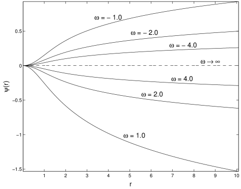
Figure 1: The numerical solution of the scalar field $\psi\equiv\ln{\epsilon}$ as a function of distance, $r$, to the core of string, for the original Bekenstein model. If $\omega<0$ then $\epsilon\to\infty$ when $r\to\infty$. On the other hand, if $\omega>0$ then $\epsilon\to 0$ when $r\to\infty$. The dashed line represents the constant-$\alpha$ theory, which corresponds to the limit $\omega\rightarrow\infty$.

It is easy to show that in the limit $\omega\,\rightarrow\,\infty$ one recovers the Nielsen-Olesen vortex with constant $\epsilon$. Although the gauge kinetic function in eqn. (24) is only well defined for $\omega>0$ the model described by the Lagrangian density in eqn. (25) allows for both negative and positive values of $\omega$. However, note that if $\omega<0$ the energy density is no longer positive definite. In Fig.1 we plot the numerical solution of the scalar field $\psi\equiv\ln{\epsilon}$ as a function of distance, $r$, to the core of string, in the context of the original Bekenstein model. Note that if $\omega<0$ then $\epsilon$ diverges asymptotically away from the string core. On the other hand if $\omega>0$ then $\psi$ goes to zero when $r\to\infty$. In the large $\omega$ limit the curves for positive and negative $\omega$ are nearly symmetric approaching the dashed line representing the constant-$\alpha$ model when $\omega\rightarrow\infty$.

3.2 Polynomial coupling

Another example of a class of gauge kinetic functions is given by

$$B_{F}(\varphi)=1.0+\sum_{i=1}^{N}\,\beta_{i}\,\varphi^{i}\,,$$ (27)

in which $\beta_{i}$ are dimensionless coupling constants and $N$ is an integer. If $\beta_{1}=0$ it is easy to verify that the classical Nielsen-Olesen vortex solution with constant $\alpha$ is still a valid solution. This means that there is a class of gauge kinetic functions for which the classical static solution is maintained despite the modifications to the model. Substituting the gauge kinetic function in eqn. (12) one gets

$$\frac{1}{r}\frac{d}{dr}(r\frac{d\varphi}{dr}) = \frac{b^{2}}{4}\left(\sum_{k=1}^{N}(2k-1)\beta_{2k-1}\varphi^{2k-2}\right)\,+$$ (28)

$$+ \frac{b^{2}}{4}\left(\sum_{k=1}^{N}(2k)\beta_{2k}\varphi^{2k-1}\right)\,.$$

which shows that the transformation $\beta_{i}\rightarrow-\beta_{i}$ for odd $i$ modifies the sign of the solution of $\varphi(r)$ without changing $\chi$ or $b$ since $B_{F}$ is kept invariant.

We will see that both for $\beta_{1}\,>\,0$ and $\beta_{1}\,<\,0$ the behaviour of $\psi\equiv\ln\epsilon$ is similar to that of the original Bekenstein model described by the lagrangian density in eqn. (25), with $\omega\,>\,0$, in particular in the limit of small $|\beta_{1}|$/large $\omega$. In fact a polynomial expansion of the exponential gauge kinetic function of the original Bekenstein model (see eqn. (24)) has $\beta_{1}=-2/{\sqrt{\omega}}$. This relation between the models arises from the fact that the exponential coupling by Bekenstein theory can be expanded in a series of powers of $\varphi$ according to

$$\beta_{i}=\frac{(-2)^{i}}{w^{i/2}i!}\,.$$ (29)

On the other hand, as mentioned before, if $\beta_{1}\,=\,0$ one recovers the standard result for Nielsen-Olesen vortex with constant-$\alpha$, independently of the chosen values of $\beta_{i}$ for $i>1$.

We have studied the behaviour of the solutions of eqns. (15-20) for various values of $N$ but for simplicity we shall only consider $N\leq 2$ in this paper. In particular, we consider

$$B_{F}=1.0+\beta_{1}\varphi+\beta_{2}\varphi^{2},$$ (30)

with two free parameters.

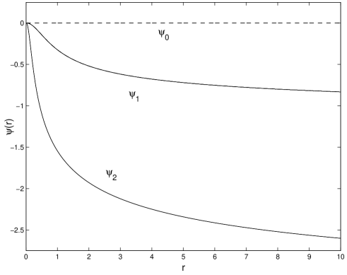
Figure 2: The numerical solution of the scalar field $\psi\equiv\ln\epsilon$ as a function of distance, $r$, to the core of string, for a polynomial gauge kinetic function. Models 0, 1 and 2 are defined by $\beta_{1}=0$ ($\beta_{2}$ arbitrary), $\beta_{1}=-3,\,\beta_{2}=0$ (linear coupling) and $\beta_{1}=-5,\,\beta_{2}=10$ respectively.

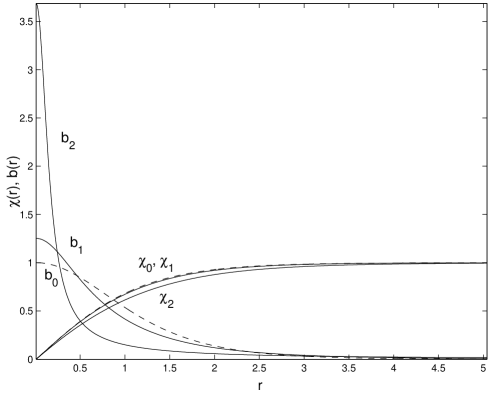
Figure 3: The numerical solution of the fields $\chi(r)$ and $b(r)$ as a function of distance, $r$, to the core of string, for models $0$, $1$ and $2$. Note that the change in $b(r)$ with respect to the standard constant-$\alpha$ result is much more dramatic than the change in $\chi(r)$.

In Fig. 2 we plot the numerical solution of the scalar field $\psi\equiv\ln\epsilon$ as a function of distance, $r$, to the core of string, for a polynomial gauge kinetic function. Models $1$ and $2$ are defined $\beta_{1}=-3,\,\beta_{2}=0$ (linear coupling) and $\beta_{1}=-5,\,\beta_{2}=10$ respectively. Model 0 (dashed line) represents any model with $\beta_{1}=0$ and has $\alpha={\rm constant}$. Note that the replacement $\beta_{1}\to-\beta_{1}$ does not modify the solution for $\psi$.

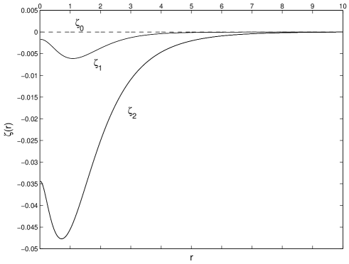
Figure 4: Plot of $\zeta_{i}(r)=\log(\chi_{i}/\chi_{0})$ for the different polynomial gauge kinetic functions. Note that although this was not very visible in Fig. 3, even a small value of $\beta_{1}$ leads to a change of the vortex solution.

In Fig. 3 we plot the numerical solution of the fields $\chi(r)$ and $b(r)$ as a function of distance, $r$, to the core of string, for models $0$, $1$ and $2$. We see that the change in $b(r)$ with respect to the standard constant-$\alpha$ result is much more dramatic than the change in $\chi(r)$. In order to verify the modification to $\chi(r)$ in more detail we define the function

$$\zeta_{i}(r)=\log\left(\frac{\chi_{i}}{\chi_{0}}\right),$$ (31)

and plot in Fig. 4 the results for the different models. We clearly see that even a small value of $\beta_{1}$ leads to a modification of the vortex solution with respect to the standard Nielsen-Olesen solution.

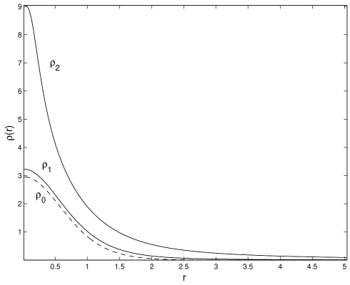
Figure 5: The energy density as a function of the distance, $r$ to the string core for models 0, 1 and 2. The dashed line represents the constant-$\alpha$ model These results clearly show an increase of the energy density due to the contribution of the extra field $\varphi$.

Finally, we have also studied the behaviour of the energy density in this model. In fact, since the fine structure constant varies we have a new contribution due to the field $\varphi$, to the total energy of the topological defect. As has been previously discussed in ref. [38] the contributions to the energy density of the string can be divided into two components. One component is localized around the string core (the local string component) the other is related to the contribution of the kinetic term associated with the spatial variations of the fine structure constant and is not localized in the core of the string. The energy profile of this last contribution is analogous to that of a global string, whose energy per unit length diverges asymptotically far from the core. In Fig. 5 we plot the string energy density as a function of the distance, $r$ to the string core for models $0$, $1$ and $2$. The dashed line represents the constant-$\alpha$ model. We clearly see an increase of the energy density due to the contribution of the extra field $\varphi$.

As an aside, let us point out that the Lagrangian density in (1) can be generalized to include a potential $V(\varphi)$. If $V(\varphi)$ has a minimum and it is steep enough near it then the spatial variations on the value of the fine structure constant can be significantly reduced. Also, if $V(\varphi)$ has more than one minimum then the Lagrangian density in (1) admits domain wall solutions which separate regions with different values of the fine structure constant. In the absence of an electromagnetic field these solutions reduce to the standard ones. On the other hand, if there are sources of electromagnetic field present (such as cosmic strings) then there may also be small fluctuations on the the value of the fine structure constant generated due to the electromagnetic source term in eqn. (7). These fluctuations are expected to be more localized due to the influence of the potential $V(\varphi)$.

4 Cosmological implications of varying-$\alpha$ strings

Having discussed in previous sections static string solutions in the context of Bekenstein-type models it is now interesting to investigate if such cosmic string networks can induce measurable space-time variations of $\alpha$ in a cosmological setting. In order to answer this question we recall that $\varphi$ satisfies the Poisson equation:

$$\nabla^{2}\varphi=\frac{1}{4}\,\beta\,f^{2}\,.$$ (32)

In eqn. (32) we have assumed for simplicity that the gauge kinetic function is a linear function of $\varphi$ with $B_{F}(\varphi)=1+\beta\varphi$. Hence the variation of the fine structure constant away from the string core is given by

$$2\pi r\frac{d\varphi}{dr}=\beta I(r)\mu(r_{\rm max})\,,$$ (33)

where

$$\mu(r)=2\pi\int^{r}_{0}\rho(r^{\prime})r^{\prime}dr^{\prime}\,,$$ (34)

and

$$I(r)=\frac{\pi}{2\mu(r_{\rm max})}\int_{0}^{r}f^{2}(r^{\prime})r^{\prime}dr^{\prime}\,,$$ (35)

is a function of $r$ smaller than unity. Here $r_{\rm max}$ represents a cut-off scale which is in a cosmological context of the order of the string correlation length. Far away from the string core $I(r)$ is a slowly varying function of $r$ which is always smaller than unity. An approximate solution for the behaviour of the field $\varphi$ may be obtained by taking $I(r)\sim{\rm const}$

$$\varphi\sim\frac{\beta I\mu(r_{\rm max})}{2\pi}\ln\left(\frac{r}{r_{0}}\right)\,,$$ (36)

where $r_{0}$ is an integration constant. Since $\epsilon=B_{F}(\varphi)^{-1/2}$ we have

$$\epsilon\sim 1-\frac{\beta^{2}I\mu(r_{\rm max})}{4\pi}\ln\left(\frac{r}{r_{0}}\right)\,,$$ (37)

We see that the variation of the fine structure constant away from the string core is proportional to the gravitational potential induced by the strings. The value of $G\mu$ is constrained to be small ($\mathrel{\hbox to0.0pt{\lower 4.0pt\hbox{\hskip 1.0pt$\sim$}\hss}\raise 1.0pt\hbox{$<$}}10^{-6}-10^{-7}$) in order to avoid conflict with CMB and LSS results [41, 42, 43, 44, 45] (or even smaller depending on the decaying channels available to the cosmic string network [46]). Note that these constraints are for standard local strings described by the Nambu-Goto action. Even though the cosmic strings studied in our paper are non-standard, having a local and a global component, we expect the limits on $G\mu(r_{\rm max})$ to be similar as those on $G\mu$ for standard local strings. On the other hand the factor $\beta$ appearing in eqn. (37) is constrained by equivalence principle tests to be $|\beta|<10^{-3}\,G^{1/2}$ [23, 39, 40]. Hence, taking into account that we cannot observe scales larger than the horizon ($\sim\,10^{4}\,{\rm Mpc}$) and are unlikely to probe variations of $\alpha$ at a distance much smaller than $1\,{\rm pc}$ from a cosmic string, eqn. (37) implies that a conservative overall limit on observable variations of $\alpha$ seeded by cosmic strings is $\Delta\alpha/\alpha\mathrel{\hbox to0.0pt{\lower 4.0pt\hbox{\hskip 1.0pt$\sim$}\hss}\raise 1.0pt\hbox{$<$}}10^{-12}$ which is too small to have any significant cosmological impact. We thus see that, even allowing for a large contribution coming from the logarithmic factor in eqn. (37), the spatial variations of $\alpha$ induced by such strings are too small to be detectable. In particular, this result means that despite the claim to the contrary in ref. [38] cosmic strings will be unable to generate inhomogeneities in $\alpha$ which could be responsible for the generation of inhomogeneous reionization scenarios.

5 Conclusion

In this article we studied Nielsen-Olesen vortex solutions in Bekenstein-type models considering models with a generic gauge kinetic function. We showed that there is a class of models of this type for which the classical Nielsen-Olesen vortex is still a valid solution (with no $\alpha$ variation). However, in general, spatial variations of $\alpha$ will be sourced by the electromagnetic energy concentrated along the string core. These are roughly proportional to the gravitational potential induced by the strings which is constrained to be small. We have shown that Equivalence Principle constraints impose tight limits on the allowed variations of $\alpha$ on cosmological scales induced by cosmic string networks of this type. As mentioned in ref. [38] other defect solutions may be considered such as monopoles or textures but in this case we expect similar conclusions to be drawn as far as the cosmological consequences of the theories are concerned. However, despite the claim in ref. [38] that domain walls can not be associated with changing-alpha theories if the scalar field $\varphi$ is endowed with a potential with a $Z_{2}$ symmetry then domain-walls may form and therefore large scale inhomogeneities in the value of $\alpha$ associated with different domains may be generated. We shall leave for future work a more detailed study of other defect solutions and cosmological implications.

References

References

- [1] J. Polchinski (1998), Cambridge, U.K.: University Press.
- [2] J. D. Barrow and C. O’Toole, Mon. Not. Roy. Astron. Soc. 322, 585 (2001), astro-ph/9904116.
- [3] J.-P. Uzan, Rev. Mod. Phys. 75, 403 (2003), hep-ph/0205340.
- [4] C. J. A. P. Martins (2003), Cambridge, U.K.: University Press.
- [5] C. J. A. P. Martins, Phil. Trans. Roy. Soc. Lond. A360, 2681 (2002), astro-ph/0205504.
- [6] J. D. Bekenstein, Phys. Rev. D25, 1527 (1982).
- [7] J. K. Webb et al., Phys. Rev. Lett. 87, 091301 (2001), astro-ph/0012539.
- [8] M. T. Murphy, J. K. Webb, and V. V. Flambaum, Mon. Not. Roy. Astron. Soc. 345, 609 (2003), astro-ph/0306483.
- [9] H. Chand, R. Srianand, P. Petitjean, and B. Aracil Astron. Astrophys. 417, 853 (2004), astro-ph/0401094.
- [10] R. Srianand, H. Chand, P. Petitjean, and B. Aracil, Phys. Rev. Lett. 92, 121302 (2004), astro-ph/0402177.
- [11] Y. Fujii, Astrophys. Space Sci. 283, 559 (2003), gr-qc/0212017.
- [12] H. Marion et al., Phys. Rev. Lett. 90, 150801 (2003), physics/0212112.
- [13] K. A. Olive et al., Phys. Rev. D69, 027701 (2004), astro-ph/0309252.
- [14] S. Hannestad, Phys. Rev D. 60, 023515 (1999), astro-ph/9810102.
- [15] P. P. Avelino et al., Phys. Rev. D64, 103505 (2001), astro-ph/0102144.
- [16] C. J. A. P. Martins et al., Phys. Rev. D66, 023505 (2002), astro-ph/0203149.
- [17] G. Rocha et al., New Astron. Rev. 47, 863 (2003), astro-ph/0309205.
- [18] C. J. A. P. Martins et al. Phys. Lett. B585, 29 (2004), astro-ph/0302295.
- [19] K. Sigurdson, A. Kurylov and M. Kamionkowski, Phys. Rev D. 68, 103509 (2003), astro-ph/0306372.
- [20] G. Rocha et al. Mon. Not. Roy. Astron. Soc. 352, 20 (2004), astro-ph/0309211.
- [21] P. P. Avelino, C. Martins, and J. Oliveira Phys. Rev. D70, 083506 (2004), astro-ph/0402379.
- [22] S. Lee, K. A. Olive, and M. Pospelov Phys. Rev. D70, 083503 (2004), astro-ph/0406039.
- [23] K. A. Olive and M. Pospelov, Phys. Rev. D65, 085044 (2002), hep-ph/0110377.
- [24] L. Anchordoqui and H. Goldberg, Phys. Rev. D68, 083513 (2003), hep-ph/0306084.
- [25] D. Parkinson, B. A. Bassett, and J. D. Barrow, Phys. Lett. B578, 235 (2004), astro-ph/0307227.
- [26] E. J. Copeland, N. J. Nunes, and M. Pospelov, Phys. Rev. D69, 023501 (2004), hep-ph/0307299.
- [27] N. J. Nunes and J. E. Lidsey Phys. Rev. D69, 123511 (2004), astro-ph/0310882.
- [28] J. L. Tonry et al., Astrophys. J. 594, 1 (2003), astro-ph/0305008.
- [29] C. L. Bennett et al. et al., Astrophys. J. Suppl. 148, 1 (2003), astro-ph/0302207.
- [30] H. B. Sandvik, J. D. Barrow, and J. Magueijo, Phys. Rev. Lett. 88, 031302 (2002), astro-ph/0107512.
- [31] D. F. Mota and J. D. Barrow, Phys. Lett. B581, 141 (2004), astro-ph/0306047.
- [32] D. F. Mota and J. D. Barrow, Mon. Not. Roy. Astron. Soc. 349, 281 (2004), astro-ph/0309273.
- [33] J. D. Barrow and D. F. Mota, Class.Quant.Grav. 20, 2045 (2003), gr-qc/0212032.
- [34] A. Albrecht and J. Magueijo, Phys. Rev D. 59, 043516 (1999), astro-ph/9811018.
- [35] J. D. Barrow and J. Magueijo, Phys. Lett. B443, 104 (1998), astro-ph/9811072.
- [36] P. P. Avelino and C. J. A. P. Martins, Phys. Lett. B459, 468 (1999), astro-ph/9906117.
- [37] P. P. Avelino and C. J. A. P. Martins, Phys. Rev D. 67, 027302 (2003), astro-ph/0209337.
- [38] J. Magueijo, H. Sandvik, and T. W. B. Kibble, Phys. Rev D. 64, 023521 (2001), hep-ph/0101155.
- [39] C. M. Will, Living Rev. Rel. 4, 4 (2001), gr-qc/0103036.
- [40] T. Damour (2003), gr-qc/0306023.
- [41] P. P. Avelino, E. P. S. Shellard, J. H. P. Wu, and B. Allen, Phys. Rev. Lett. 81, 2008 (1998), astro-ph/9712008.
- [42] J. H. P. Wu, P. P. Avelino, E. P. S. Shellard and B. Allen, Int. J. Mod. Phys. D11, 61 (2002), astro-ph/9812156.
- [43] R. Durrer, M. Kunz, and A. Melchiorri, Phys.Rept. 364, 1 (2002), astro-ph/0110348.
- [44] P. P. Avelino and Liddle, Mon. Not. Roy. Astron. Soc. 348, 105 (2004), astro-ph/0305357.
- [45] J.-H. P. Wu, (2005), astro-ph/0501239.
- [46] P. P. Avelino and D. Barbosa, Phys. Rev D. 70, 067302 (2004), astro-ph/0406063.