Night sky brightness at sites from DMSP-OLS satellite measurements
Abstract
We apply the sky brightness modelling technique introduced and developed by Roy Garstang to high-resolution DMSP-OLS satellite measurements of upward artificial light flux and to GTOPO30 digital elevation data in order to predict the brightness distribution of the night sky at a given site in the primary astronomical photometric bands for a range of atmospheric aerosol contents. This method, based on global data and accounting for elevation, Earth curvature and mountain screening, allows the evaluation of sky glow conditions over the entire sky for any site in the World, to evaluate its evolution, to disentangle the contribution of individual sources in the surrounding territory, and to identify main contributing sources. Sky brightness, naked eye stellar visibility and telescope limiting magnitude are produced as 3-dimensional arrays whose axes are the position on the sky and the atmospheric clarity. We compared our results to available measurements.
keywords:
atmospheric effects – site testing – scattering – light pollution1 Introduction
The change in the light in the night environment due to the introduction of artificial light is a true pollution, a growing adverse impact on the night. Pollution means ”impairment or alteration of the purity of the environment” or of its chemical/physical parameters. This alteration of natural light at night, called light pollution, can and does impact the environment and the health of the beings living in it (animals, plants and man), as shown by hundreds of scientific studies and reports (see e.g. Rich & Longcore 2002, Erren & Piekarski 2002, Cinzano 1994). The growth of the night sky brightness is one of the many effects of artificial light being wasted in the environment. It is a serious problem. It endangers not only astronomical observations but also the perception of the Universe around us (see Crawford (1991), Kovalewski (1992), McNally (1994), Isobe & Hirayama (1998), Cinzano (2000a), Cohen & Sullivan (2001), Cinzano (2002), Schwarz (2003) and the International Dark-Sky Association Web site, www.darksky.org). The starry sky constitutes mankind’s the only window to the universe beyond the Earth. A fundamental heritage for the culture, both humanistic and scientific, and an important part of the our nighttime landscape patrimony is going to be lost, for those alive today and for our children and their children. The worldwide growing interest for light pollution and its effects requires methods for monitoring this situation.
The modelling of the brightness distribution of the night sky at a site is important to evaluate its suitability for astronomical observations, to quantify its sky glow, and to recognize endangered parts of the sky hemisphere. Night sky models are useful in studying sky glow relationships with atmospheric conditions and to evaluate future changes in sky glow. The modelling is also required to disentangle the contribution of sources, such as individual cities, in order to recognize those areas producing the strongest impact and to undertake actions to limit light pollution.
In 1986 Roy Garstang introduced a modelling technique, developed and refined in the subsequent years (Garstang 1986, 1987, 1988, 1989a, b, 1991a, b, c, 1992, 1993, 2000a), to compute the light pollution propagation in the atmosphere. He estimated the night sky brightness at many sites based on the geographical positions, altitudes and populations of the polluting cities. Cinzano (2000b) used Garstang models to disentangle the impact of individual cities constraining free functions with the condition that the sum of all the contributions with the natural sky brightness fits the observed sky brightness. However updated population data are not easily available worldwide, the upward light emission is not strictly proportional to the population. Some polluting sources, such as industrial areas and airports, have very low population density but very high light emission. The U.S. Air Force Defence Meteorological Satellite Program (DMSP), Operational Linescan System (OLS) acquires direct observations of nocturnal lighting, making it possible to map the spatial distribution of nighttime lights (Sullivan 1989, 1991; Elvidge et al. 1997a, b, c, 2001, 2003a, b; Gallo et al. 2003; Henderson et al. 2003). Most nighttime OLS observations of urban centers are saturated, making the data of limited value for modeling purposes. However, Elvidge et al. (1999) were able to produce a radiance calibrated global nighttime lights product using OLS data acquired at reduced gain settings, suitable for the quantitative measurement of the upward light emission (e.g. Isobe & Hamamura 2000, Luginbuhl 2001, Osman et al. 2001) and the evaluation of the artificial sky brightness produced by it (e.g. Falchi 1998; Falchi & Cinzano 2000).
Cinzano et al. (2000) presented a method to map the artificial sky brightness across large territories in a given direction of the sky by evaluating the upward light emission from DMSP high resolution radiance calibrated data (Elvidge et al. 1999) and the propagation of light pollution with Garstang models. A World Atlas of the artificial night sky brightness at sea level was thus obtained (Cinzano, Falchi & Elvidge 2001b). This method was extended by Cinzano, Falchi & Elvidge (2001a) to the mapping of naked eye and telescopic limiting magnitude based on the Schaefer (1990) and Garstang (2000b) approach and the GTOPO30 elevation data. We extend and apply their method to the computation of the distribution of the night sky brightness and the limiting magnitude over the entire sky at any site for a range of atmospheric conditions and accounting for mountain screening. In sec. 2 we describe the computation on 3-dimensional arrays whose axes are the position on the sky and the atmospheric clarity and present our improvements. In sec. 3 we describe input data. In sec. 4 we deal with the disentangling of individual sources. In sec. 5 we discuss the application and in sec. 6 we present comparisons with available measurements. Conclusions are in sec. 7.
2 Computation of the Hypermaps
Artificial and natural sky brightness varies depending on the aerosol content of the atmosphere. The stellar extinction also vary substantially depending on the aerosol content of the local atmosphere. This in turn affects the limiting magnitude. So any map of the sky of a site is a function of the aerosol content for which it has been computed.
We refer to a hyper-map as a set of maps of the night sky brightness for a range of aerosol contents, , where is the zenith distance, is the azimuth and is the aerosol content expressed by the atmospheric clarity (Garstang 1986, 1989). As fig. 1 shows, values on planes of the space of the variables perpendicular to the axis give maps of the sky brightness for the given atmospheric clarity, values along a line parallel to the axis give the brightness in the given point of the sky when the atmospheric aerosol content change, values along lines perpendicular to the and axis give the sky brightness along an almucantar for the given atmospheric clarity.
At a site in the hyper-map is given by:
| (1) |
where is the light pollution propagation function, i.e. the artificial sky brightness at in the direction given by per unit of upward light emission produced by the unitary area in when atmospheric aerosol content is K. If we divide a territory in land areas with position , the hyper-map can be expressed as a tridimensional array given by:
| (2) |
where is the upward flux emitted by the land area , is the propagation function, are an adequate discretization of the variables and the sommatories are extended at all the land areas around the site inside a distance for which their contributions are non negligible. We divided the territory in the same land areas covered by pixels of the satellite data. We obtained the propagation function , expressed as total flux per unit area of the telescope per unit solid angle per unit total upward light emission, with models for the light propagation in the atmosphere based on Garstang models (Garstang 1986, 1989):
| (3) |
where are respectively the scattering cross sections of molecules and aerosols per unit volume at the altitude , depending on the distance along the line of sight of the observer, and are their normalized angular scattering functions (see sec.3.3), is the scattering angle, is the extinction of the light along its path from the scattering volume to the telescope, is the direct illuminance per unit flux produced by each source on each infinitesimal volume of atmosphere along the line-of-sight and is a correction factor which take into account the illuminance due at light already scattered once from molecules and aerosols which can be evaluated as Garstang (1984, 1986), neglecting third and higher order scattering which can be significant for optical thickness higher than about 0.5. Geometric relations and formulae accounting for Earth curvature have been given and discussed by Garstang (1989, sec. 2.2-2.5, eqs. 4-24). In Garstang’s formulae the molecular scattering cross section per unit volume is .
As Garstang (1989) and differently from Cinzano et al. (2001a) we take into account the elevation both of the source and of the site.
Screening by terrain elevation was accounted as described in Cinzano et al. (2001a). The illuminance per unit flux was set in eq. (3) to:
| (4) |
where there is no screening by Earth curvature or by terrain elevation and elsewhere. Here is the normalized emission function giving the relative light flux per unit solid angle emitted by each land area at the zenith distance , is the distance between the source and the considered infinitesimal volume of atmosphere and is the extinction along the light path, given by Garstang (1989). We check each point along the line of sight to determine if the source area is blocked by terrain elevation or not, taking into account Earth curvature, by determining the position of the foot of the vertical of the considered point. Then we computed for every land area crossed by the line connecting this foot and the source area, the quantity (Cinzano et al. 2001a):
| (5) |
where is the elevation of the land area, is the distance of its center from the center of the source area and is the Earth radius. From it we determined the screening elevation :
| (6) |
where is the distance between the source area and the foot of the vertical, and is computed over the sea level. The illuminance in eq. (3) is set to zero when the elevation of the considered point is lower than the screening elevation. To speed up the calculation we computed only once the array, which gives the screening elevation for each point along the line of sight, for each azimuth of the line of sight and for each source, and we used it for any computation with different atmospheric parameters. We considered land areas as point sources located in their centres except when , in which case we used a four points approximation (Abramowitz & Stegun 1964). We assumed that the elevation given by the GTOPO30 be the same everywhere inside each pixel.
Another array was obtained for the natural sky brightness with the model introduced by Garstang (1989, sec. 3). The array is the sum of (i) the directly transmitted light which arrives to the observer after extinction along the line of sight (Garstang 1989, eq. 30), (ii) the light scattered by molecules by Rayleigh scattering (Garstang 1989, eq. 37), (iii) the light scattered by aerosols (Garstang 1989, eq. 32) :
| (7) |
In the computation of the natural sky brightness outside the scattering and absorbing layers of the atmosphere (Garstang 1989, eq.29) we assumed as independent variables the brightness of a layer at infinity, due mainly to integrated star light, diffused galactic light and zodiacal light, and the brightness of the van Rhijn layer, due to airglow emission.
The array of the total sky brightness is . The sky brightness in the chosen photometric band was expressed as photon radiance (in ph cm-2 s-1 sr-1) or in magnitudes per arcsec2 (Garstang 1989, eqs. 28, 39).
We determined the observer’s horizon computing the altitudes below which the line-of-sight encounter a screen by terrain, like e.g. a mountain, and set the total brightness to be zero below them. They are obtained evaluating the elevation of terrain at distance along each azimuth direction and computing the maximum screening altitude angle :
| (8) |
From the array of the total sky brightness in V band we can obtain a family of other arrays giving the naked-eye star visibility and the telescopic limiting magnitude. The magnitude over the atmosphere of a star at the threshold of visibility of an observer when the brightness of observed background is in nanolambert and the stimulus size, i.e. the seeing disk diameter, is in arcmin, has been given by Garstang (2000b) based on measurements of Blackwell (1946) and Knoll, Tousey & Hulburt(1946) and on a threshold criterion of 98 per cent probability of detection:
| (9) |
with:
| (10) | |||||
| (11) | |||||
| (12) | |||||
| (13) |
where and are the illuminations produced by the star, related respectively to the thresholds of scotopic and photopic vision, and the fraction is an artifact introduced by Garstang in order to put together smoothly the two components obtaining the best fit with cited measurements. Here takes into account the ratio between pupil areas of the observer and the pupil diameter used by the average of the Knoll, Tousey, Hulburt and Blackwell observers, takes into account the Stiles-Crawford effect, due to the decreasing of the efficiency to detect photons with the distance from the center of the pupil, producing a non linearity in the increase of sensibility when the eye pupil increase, allows for the difference in color between the laboratory sources used in determining the relationships between and and the observed star, allows for star light extinction in the terrestrial atmosphere because star magnitudes are given outside the atmosphere, allows for the acuity of any particular observer, defined so that implies an eye sensitivity higher than average due possibly to above average retinal sensitivity, scientific experience or an above average eye pupil size. Formulae have been given by Schaefer (1990) and Garstang (2000b) and applied by Cinzano et al. (2001a, eqs. 28-31) to which we refer the reader. The constants , , , , in eq. (10) are given by Garstang (2000b). The perceived background is related to the total sky brightness under the atmosphere in band given by our hyper-maps, converted from photon radiance to nanolambert (Garstang 2000b):
| (14) |
where allow for the difference in color between the laboratory sources and the night sky background, and were already described. As a result we obtain the array of the visual limiting magnitude. The array of the telescopic limiting magnitudes can be calculated for the chosen instrumental setup in a similar way (see the cited authors).
3 Input data
We summarize here the required input data, which has been already described and discussed by Cinzano et al. (2000, 2001a). We refer the reader to their paper for details. We extended the input data to other continents in the same way.
3.1 Upward light emission data
To compute the illuminance per unit flux in eq. 4 we need the relative intensity emitted by every land area in at azimuth and zenith distance , i.e. the normalized emission function obtained measuring the relative emitted flux per unit solid angle per unit area in the direction and normalizing its integral to unity. If the land areas contain many light installations randomly distributed in type and orientation, we can assume this function axysimmetric . The corresponding absolute intensity is:
| (15) |
where is the total upward flux obtained from radiance calibrated data (Cinzano 2001a, eq. 35).
We obtained the upward flux on a 30”30” pixel size grid from the Operational Linescan System (OLS) carried by the DMSP satellites after a special requests to the U.S. Air Force made by the U.S. Department of Commerce, NOAA National Geophysical Data Center (NGDC), which serves as the archive for the DMSP and develops night time lights processing algorithms and products. OLS is an oscillating scan radiometer with low-light visible and thermal infrared (TIR) high-resolution imaging capabilities (Lieske 1981). The OLS Photo Multiplier Tube (PMT) detector has a broad spectral response covering the range for primary emissions from the most widely used lamps for external lighting. The primary reduction steps were (Cinzano et al. 2000, 2001a; Elvidge et al. 1999):
-
1.
1) acquisition of special OLS-PMT data at a number of reduced gain settings to avoid saturation on major urban centres and, in the same time, overcome PMT dynamic range limitation. On board algorithms which adjust the visible band gain were disabled.
-
2.
establishment of a reference grid with finer spatial resolution than the input imagery;
-
3.
identification of the cloud free section of each orbit based on OLS-TIR data;
-
4.
identification of lights, removal of noise and solar glare, cleaning of defective scan lines;
-
5.
projection of the lights from cloud-free areas from each orbit into the reference grid;
-
6.
calibration to radiance units using preflight calibration of digital numbers for given input telescope illuminance and gain settings in simulated space conditions;
-
7.
tallying of the total number of light detections in each grid cell and calculation of the average radiance value;
-
8.
filtering images based on frequency of detection to remove ephemeral events;
-
9.
transformation into latitude/longitude projection with 30”30” pixel size;
-
10.
Lucy-Richardson deconvolution to improve predictions for sites near sources (when possible this should be more properly done before step 7).
-
11.
Determination of the upward light intensity accounting for the estimated atmospherical extinction in the light path from ground to the satellite, the assumed average spectrum of night-time lighting (Cinzano et al. 2000a, eqs. 28-30) and the surface of the land areas.
We can obtain from the radiance measured in a set of individual orbit satellite images where the land area in is seen at different angles which are related to the distance from the satellite nadir (Cinzano et al. 2000, eq. 17, 18). The emitted flux per solid angle per unit area in the direction is obtained from the measured radiance dividing by the extinction coefficient computed for curved-Earth (Cinzano et al. 2000, eq. 19). A study to obtain in this way for every land area from DMSP-OLS individual orbit data is in progress (Cinzano, Falchi, Elvidge, in prep.). To be simple we assumed here that all land areas have in average the same normalized emission function, given by the parametric representation of Garstang Garstang (1986) in eq. (15) of Cinzano et al. (2000), which has been tested by studying in a single orbit satellite image the relation between the upward flux per unit solid angle per inhabitant of a large number of cities and their distance from the satellite nadir (Cinzano et al. 2000) and with many comparisons between model predictions and measurements by Garstang and by Cinzano (2000b). Likely it cannot be applied in areas where effective laws against light pollution are enforced or with unusual lighting habits.
3.2 Elevation data
As input elevation data we used GTOPO30, a global digital elevation model by the U.S. Geological Survey’s EROS Data Center (Gesch et al. 1999). This global data set covers the full extent of latitude and longitude with an horizontal grid spacing of 30” as our composite satellite image. The vertical units represent elevation in meters above mean sea level which ranges from -407 to 8,752 meters. We reassigned a value of zero to ocean areas, masked as ”no data” with a value of -9999, and to altitudes under sea level.
3.3 Atmospheric data
In order to evaluate scattering and extinction we need a set of functions giving, for each triplet of longitude, latitude and elevation , the molecular and aerosol cross scattering coefficients per units volume of atmosphere and , and the aerosol angular scattering function . The molecular angular scattering function is known because it is Rayleigh scattering. The atmospheric data need to refer at a typical clean night in the chosen time of the year and to include information on denser aerosol layers, volcanic dust and Ozone layer.
To be simple we applied here the standard atmospheric model already adopted by Garstang (1986, 1989) and Cinzano et al. (2000, 2001a), neglecting geographical gradients and local particularities. It assumes:
-
1.
the molecular atmosphere in hydrostatic equilibrium under the gravitational force as Garstang (1986).
-
2.
the atmospheric haze aerosols number density decreasing exponentially as Garstang (1986)
-
3.
a neglegible presence of sporadic denser aerosol layers, volcanic dust and Ozone layer (studied by Garstang 1991a, c).
-
4.
the normalized angular scattering function for atmospheric haze aerosols given in Garstang (1991a).
-
5.
the aerosol content given by an atmospheric clarity parameter which measures the relative importance of aerosol and molecules for scattering light.
The Garstang atmospheric clarity parameter measures the relative importance of aerosol and molecules for scattering light in band at ground level (Garstang 1996):
| (16) |
where is the altitude of the ground level over sea level and is the inverse scale height of molecules. It assumes that there is only one ground level where all the polluting sources lie. To be more self-consistent when there are many cities at different elevations over sea level, we introduced an atmospheric clarity parameter defined at sea level:
| (17) |
so that at ground level of each city , where is the inverse scale height of aerosols. We can associate the atmospheric clarity K with vertical extinction (e.g. Garstang 1991, eq. 6) and with other observable quantities like the horizontal visibility (Garstang 1989, eq. 38), the optical thickness (Garstang 1986, eq. 22) and the Linke turbidity factor for total solar radiation (Garstang 1988). Extinction along light paths for this atmospheric model was given by Garstang (1989, eqs. 18-22).
3.4 Natural night sky brightness data
The brightness , due to integrated star light, diffused galactic light and zodiacal light, depends on the observed area of the sky and on the time. This dependence on the position of the sky is important when sky maps are made to quantify the visibility of astronomical phenomena, otherwise we can assume constant and given by its average value in the considered site. The brightness of the Van Rhijn layer, , depends on some factors like the geographical position, the solar activity in the previous day, and the time after twilight. We referred our predictions to some hours after the twilight, when the night brightness decay at a constant value (Walker 1988, but see also Patat 2003a), and to minimum solar activity. If requested, the solar activity can be roughly accounted as Cinzano et al (2001a) or, more accurately, based on the correlation with the 10.7 cm solar radio flux (Walker 1988, Krisciunas 1999). The dependence of by the geographical position suggests to study the natural sky brightness in the nearest unpolluted site, which can be located in the world atlas of artificial sky brightness (Cinzano et al. 2001b), in order to obtain and . When only one or few measurements were available we assumed as Garstang (1989) and and determined .
4 Disentangling individual contributions
We can make some analysis on the contributions from each 30”30” land area which enter in the summatory of eq.(2). First we can make hypermaps of sky brightness produced by individual land areas and compare them. Moreover, chosen an array cell of index we can obtain a geographic map showing the contribution produced by each land area in , searching for main polluting sources and making some statistic on their geographic distribution:
| (18) |
We can obtain hypermaps of sky brightness produced by each city or territory identifying pixels belonging to each city or territory of a given list and summing their contributions:
| (19) |
Their comparison is helpful e.g. to understand if larger contributions come from few main cities or from many small towns, even in relation with atmospheric conditions. The fraction of sky brightness produced in a given array cell by the sources inside a circular area of radius can be obtained summing all contributions of land areas inside the distance from the site and dividing by the sum of all contributions:
| (20) |
This is useful e.g. to evaluate the effectiveness of protection areas (Cinzano 2000c).
5 Application
The software package lpskymap, written in Fortran-77, calculates the artificial night sky brightness, the total night sky brightness and the star visibility (limiting magnitude) over the entire sky at any site in the World. The availability of OLS-DMSP fixed gain data on a yearly or sub-yearly timescale will allow a fine time resolution.
Results are arrays of the artificial night sky brightness, the total night sky brightness, the visual limiting magnitude and the loss of visual limiting magnitude. Each hyper-map array is composed by a series of 1937 pixel images in cartesian coordinates, one for each aerosol content , spline interpolated over 91181 pixels in cartesian coordinates or projected in 721721 pixels in polar coordinates. Images go from 0 to 360 degrees in azimuth, starting from East (in order to avoid to place the meridian at borders) toward South, and from horizon to zenith in altitude. They are saved in 16-bit standard fits format with fitsio Fortran-77 routines developed by HEASARC at the NASA/GSFC. ASCII data tables are also provided. The night sky brightness in the chosen photometric band is given as photon radiance in ph s-2 m-2 sr-1 or as astronomical brightness in mag arcsec-2. Brightness in V band can be also expressed as luminance in cd m-2, using Garstang’s conversion (Garstang 2002; Cinzano 2004). From the hyper-map arrays we can obtain:
-
1.
sections perpendicular to the axis: . They are the maps of the sky brightness or limiting magnitude for a given aerosol content and they correspond to each individual image of the series.
-
2.
secants parallel to the axis: . They provide the brightness or the limiting magnitude in a given point of the sky as the aerosol content changes.
-
3.
secants perpendicular to the and axis: . They give the brightness or the limiting magnitude along an almucantar, e.g. the meridian, for a given aerosol content.
The arrays computation steps are:
-
1.
An input file is prepared with the geographical position and elevation of the site, the names of input DEM and lights frames and the position of their upper left corner.
-
2.
The array, i.e. the series of images, of the artificial night sky brightness is computed with the program lpskymap for a given range and step of the aerosol content, accounting for Earth curvature and elevation but not for screening. The radius of the contributing area can be 250 km for sites in urbanized areas or 350 km for dark sites.
-
3.
Subimages with DEM and lights data have been cropped from the original large scale frames with the program makefrac. We use fits or raw images 701x701 px in size to limit the requirements of RAM memory during screening computation. They are checked for relative mismatches which can be corrected with the program makeshift.
-
4.
The screening angles for each direction of observation and for each area inside a given radius from the site are computed with the program makescreen. We limited the radius to 200 km to avoid too long computation time. The program writes the screening data of each site in 106 files for a total size of 20GB uncompressed. It also calculates the horizon line as seen by the site. DEM pixels very near to the site are divided in 11x11 sub pixels evaluated separately.
-
5.
An array containing the screened brightness is computed with the program lpskyscreen when there are reasons to believe that screening is not negligible.
-
6.
The images of the screened brightness array are subtracted from the correspondent images of the sky brightness array, after properly rescaling, in order to obtain the array of the night sky brightness corrected for mountain screening.
-
7.
The array is calibrated with the program lpskycal based on pre-flight calibration at 1996-1997, or on Cinzano et al. (2001b) calibration at 1998-1999 made with Earth-based measurements, or on observations taken at the same site. Measurements of Cinzano et al. (2001a) fitted predictions based on the pre-flight calibration with 0.35 mag arcsec-2 and a shift =-0.28 mag arcsec-2, likely mainly due to the growth of light pollution in the period between the observations and the satellite data acquisitions. The program adds the natural sky brightness, producing a series of calibrated maps of the total night sky brightness, interpolated or not, and the limiting magnitude. It also adds the horizon line. It does not account for the refraction of light by the atmosphere which could increase the brightness near the horizon toward very far cities.
-
8.
Maps in polar coordinates are obtained with the program lpskypolar. East is up, North at right.
-
9.
Maps are analyzed with ftools developed by HEASARC at the NASA/GSFC.
-
10.
Comparison with observations is made with the program lpskycompare. Measurements should be ”under the atmosphere”. Statistical analysis is made with the software mathematica of Wolfram Research.
A number of utility programs completes the package. The computation time depends on the geographical behavior of the site, like the quantity of dark pixels, the quantity of nonzero elevation pixels, etc. As an example, the computation of one element of the array (i.e. a single map for a given atmospheric content) for Sunrise Rock on a workstation with Xeon processor running at 1700 MHz required about 35 hours for lpskymap, 10 hours for makescreen and 6 hours for lpskyscreen. However, the computation with lpskymap for the site in Padua required 80 hours, even if restricted inside a radius of 250 km, whereas the same computation for Serra La Nave required 18 hours only.
6 Results
In this section we present a sample of results which can be obtained with our method and some comparisons with available measurements. Specific studies are reserved for forthcoming papers.
NGDC request for low and medium gain DMSP-OLS data used in this work was granted from U.S. Air Force for the darkest nights of lunar cycles in March 1996 and January-February 1997. More recent data sets taken in the period 1999-2003 are already at our disposal, but they are still under reduction and, before we are able to use them, we need to solve a number of problems in the analysis process (Cinzano, Falchi & Elvidge, in prep.). Pre-flight calibration of upward flux refers to 1996-1997, to the average lighting spectra of Cinzano et al. (2000) and to an average vertical extinction in V band at imaging time assumed to be mag. All results are computed for minimum solar activity and refers to some hours after twilight. We tuned the parameter to fit the zenith natural sky brightness for clean atmosphere measured by Cinzano et al. (2001a) at Isola del Giglio, Italy, mag arcsec-2 in V band for average solar activity and 200 m altitude over sea level. It agrees well with the average natural night sky brightness of 21.6 mag arcsec-2 measured by Patat (2003a) at ESO-Paranal. In facts, the sky become darker going to lower elevation over sea level due to larger extinction, even if this phenomena is limited by the increase of the light scattered from aerosols and molecules along the line of sight (Garstang 1989). Patat (2003) reported a large contribution from zodiacal light, about 0.18 mag arcsec-2, which justifies the fact that he finds the sky slightly more luminous than expected. The algorithm of Patat (2003b) applied to VLT images excludes almost completely the stellar component whereas Cinzano et al. (2001a) excluded only stars fainter than 18th mag, but the expected difference is only 0.03 mag arcsec-2. The ”visual” natural night sky brightness should be obtained from the measured one adding the average stellar background produced by stars with magnitude 7 missed by the instrument or the analysis (Cinzano & Falchi 2004). This contribute is about -0.26 mag arcsec-2 when stars down to magnitude 24 are missed. In our brightness predictions we did not correct the natural night sky brightness to the visual value.
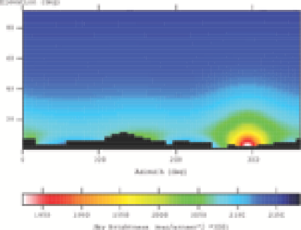
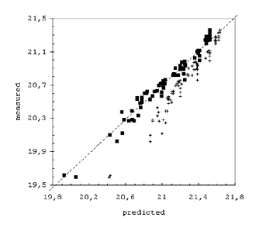
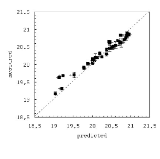
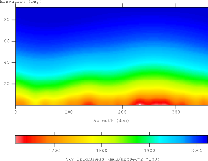
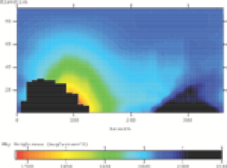
Fig. 2 shows the night sky brightness at Sunrise Rock, a site located in Mojave National Preserve, California, USA (long W 115 33’ 6.4”, lat N 35 18’ 57.7”) at 1534 m over sea level. This site is mainly polluted by the lights of Las Vegas, about 100 km away. Azimuth goes from 0 to 360 degrees, starting from East toward South. Fig. 3 shows the night sky brightness screened by mountains, which amounts to few hundredth of magnitude. Fig. 4 shows a comparison between predictions for atmospheric clarities =0.5 (squares) or =3 (crosses) and V band measurements taken on 2003 May 8 at 05.34-06.00 UT (Duriscoe et al. 2004) with vertical extinction kV=0.18 mag. The agreement is excellent after an uniform scaling of about -0.3 mag arcsec-2. It suggests an increase of light pollution from 1997 to 2003 of 5 per cent per year, slightly less than the average yearly growth 6 per cent estimated by Cinzano (2003). A comparison with a data set taken on 2003 September 22 at 06.27-06.58 UT with kV=0.26 mag gives similar results.
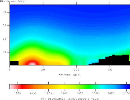
Fig. 5 shows the night sky brightness at Serra la Nave Observatory (long E 14 58’ 24”, lat N 37 41’ 30”) at 1734 m over sea level on the Mt. Etna volcano, Italy. This site is situated at few kilometers from a densely populated area with 1.8 106 inhabitants, which includes the cities of Catania (23 km) and Messina (75 km). Fig. 6 shows a comparison between predictions for atmospheric clarities =1 (squares) and =2 (crosses) with V band measurements taken on 1998 February 22-23 at 18.00-20.00 UT with vertical extinction kV=0.26 mag (Catanzaro & Catalano 2000; see fig. 2). The agreement is good. The fit is slightly better for the model with =1, corresponding to a vertical extinction of kV=0.17 mag, which is smaller than the measured one. However the vertical extinction at this site could be locally determined by the volcanic dust (Catanzaro, priv. comm.) whereas depends on the average aerosol content of the entire area with 250 km radius, so they do not need to match.
The effect of an increase of the aerosol content depends on the distribution of sources around the site. In general it decreases the zenith brightness when the distance of the main sources is larger than few kilometers, decreases the brightness at low elevation in direction of far sources, increases the brightness at very low elevation in direction of sources at small or average distance. This could explain the different behavior of the sky brightness with the aerosol content in these two sites.
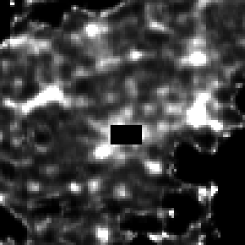
Fig. 7 shows the night sky brightness versus the zenith distance at G. Ruggeri Observatory, Padova, Italy (long E 11 53’ 20”, lat N 45 25’ 10”). This site is located inside a city of 8 inhabitants in a plain with more than 4 inhabitants. Positive zenith distances collect measurements with azimuth inside 90 from the direction of the city centre. Open symbols are the V band measurements taken on 1998 March 26 at 20.00-23.30 UT, with kV=0.48 mag (Favero et al 2000). Filled symbols are predictions in the same directions for atmospheric clarity =3, corresponding to kV=0.65 mag. For smaller values of the brightness is underestimated by a constant value. This is likely due to the fact that our model cannot accurately account for the scattered light coming from lighting installations inside few hundreds of meters from the site because pixel sizes are of the order of 1 km. We used for this prediction the calibration made for 1998-1999 by Cinzano et al. (2001a). For an atmospheric clarity , i.e. for an optical depth , the double scattering approximation could be not fully adequate (Garstang 1989; Cinzano et al. 2000). Fig. 8 shows the contribution to the artificial night sky brightness produced in the same site from the sources outside Padua for atmospheric clarity 1.9 (kV=0.48 mag). The area neglected in the prediction is shown in Fig. 9 together with the distribution of lights in the Padana Plain surrounding Padua from OLS-DMSP satellite data.
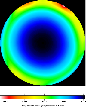
Fig. 10 shows in polar coordinates the total night sky brightness in V band at Mt. Graham Observatory, USA (long W 109 53’ 31”, lat N 32 42’ 5”, 3191m o.s.l.) for atmospheric clarity . It can be compared with the image available at the web address http://mgpc3.as.arizona.edu/images/ Night%20Sky%20large.jpg or with fig. 8 of Garstang (1989), which shows only the artificial brightness.
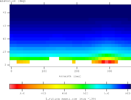
Fig. 11 shows the naked eye limiting magnitude at Sunrise Rock. Limiting magnitude is computed for observers of average experience and capability , aged 40 years, 98 per cent detection probability (faintest star that the observer sees surely and not the faintest suspected star) and star color index = 0.7 mag. Experienced amateur astronomers are more trained in naked-eye observation than unexperienced peoples and can consider detected a star at a much smaller detection probability so that their limiting magnitude can be more than one magnitude larger (Schaefer 1990). See the discussion in Cinzano et al. (2001a).
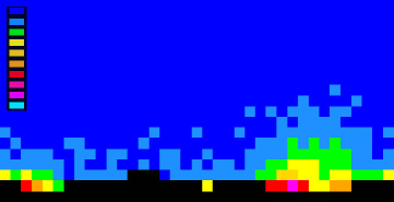
We checked the effects of the mountain screening trying to reproduce the umbrae on the sky modelled by Schaefer (1988) and due to the screening produced by the Mauna Kea on the light of the rising sun backscattered to the observer. Fig. 12 shows the analogous of the Schaefer’s umbrae produced by a source of light pollution instead of the Sun. A city screened by a large conic mountain (left) projects an umbra over the horizon (right). When the mountain is off-set in respect to the line observer-source, a non symmetric penumbra appears. Here the penumbra is at higher altitudes than in the Wynn-Williams’ photo (Schaefer 1988, fig.1) likely because the observer is at lower elevation. Further examples of umbrae and baffles are shown by Cinzano & Elvidge (2003a fig.1 and fig.3, 2003b).
7 Conclusions
We extended the seminal works of Garstang by applying his models to upward flux data from DMSP satellites and to GTOPO30 digital elevation models, and by accounting for mountain screening. The presented method allows one to monitor the artificial sky brightness and visual or telescopic limiting magnitudes at astronomical sites or in any other site in the World.
This study provides fundamental information in evaluating observing sites suitable for astronomical observations, to quantify sky glow, to recognize endangered parts of the sky hemisphere when measurements are not readily available or easy feasible, and to quantify the ability of the resident population to perceive the Universe they live in. The method enables to study the relationship of night sky brightness with aerosol content and to evaluate its changes with time. The method also allows one to analyze the adverse impacts on a site from the surrounding territories, making it possible to disentangle individual contributions in order to recognize those that are producing the stronger impact and hence to undertake actions to limit light pollution (the use of fully shielded fixtures, limitation of the downward flux wasted outside the lighted surface, use of lamps with reduced scotopic emission, flux reduction whenever possible, no lighting where not necessary, restraining of lighting growth rates or lighting density, etc). We also present some tests of the method. The effects of light pollution on the night sky are easily evident in the maps in the text.
Important refinements needs to be done in the future years: i) it may be possible to derive the angular distribution of light emissions from major sources of nighttime lighting from OLS or future satellite data (Cinzano, Falchi, Elvidge in prep.). This will improve accuracy of the modelling, in particular where laws against light pollution are enforced; ii) a global Atlas of the growth rates of light pollution and zenith night sky brightness from satellite data (Cinzano, Falchi, Elvidge in prep.) will make it possible to predict the evolution of the night sky situation at sites; iii) a worldwide atmospheric data set giving the atmospheric conditions in any land area for the same nights of satellite measurements or for a typical local clear night will allow to replace the standard atmosphere with the true atmosphere or the typical local atmosphere; iv) the availability of spectra of the light emission of each land area from satellite will allow a more precise conversion of OLS data to astronomical photometrical bands and an accurate modelling of the colors of the night sky; v) a large number of accurate measurements of night sky brightness and visual limiting magnitude including the evaluation of the atmospheric content, from e.g. the vertical extinction, will allow to better constrain predictions allowing improvements of the modelling technique. The International Dark-Sky Association, the organization which takes care of the battle against light pollution and the protection of the night sky is making a large worldwide effort to collect accurate measurements of both night sky brightness and stellar extinction (e.g. Cinzano & Falchi 2004). They constitute a fundamental component of the monitoring of the night sky situation in the World.
Acknowledgments
We are indebted to Roy Garstang of JILA-University of Colorado for his friendly kindness in reading this paper, for his helpful suggestions and for interesting discussions. We acknowledge the EROS Data Center, Sioux Falls, USA for kindly providing us their GTOPO30 digital elevation model and the National Park Service Night Sky Team, Death Valley, USA, together with the authors Dan Duriscoe, Chad Moore, and Christian Luginbuhl, for kindly providing us some of their night sky brightness data. This work has been supported by the Italian Space Agency contract I/R/160/02. The application to Padua is part of a research project supported by the University of Padua CPDG023488.


References
- Abramovitz & Stegun (1964) Abramovitz M., Stegun I.A., 1964, Handbook of Mathematical Functions. NBS, Washington
- Blackwell (1946) Blackwell H. R., 1946, J. Opt. Soc. Am., 36, 624
- Catanzaro & Catalano (2000) Catanzaro G., Catalano F.A., 2000, in Cinzano P., ed., Measuring and Modelling Light Pollution, Mem. Soc. Astron. Ital., 71, 211-220
- Cinzano (1994) Cinzano P., 1994, References on Light Pollution and Related Fields, Part D, Int. Rep. No.11, Dep. Astron., University of Padova, http://dipastro.pd.astro.it/cinzano/ refer/node8.html
- Cinzano (2000a) Cinzano P., ed., 2000a, Measuring and Modelling Light Pollution, Mem. Soc. Astron. Ital., 71
- Cinzano (2000b) Cinzano P., 2000b, in Cinzano P., ed., Measuring and Modelling Light Pollution, Mem. Soc. Astron. Ital., 71, 113-130
- Cinzano (2000c) Cinzano P., 2000c, in Cinzano P., ed., Measuring and Modelling Light Pollution, Mem. Soc. Astron. Ital., 71, 93-112
- Cinzano (2002) Cinzano P., ed., 2002, Light Pollution and the Protection of the Night Environment, Proceedings, ISTIL, Thiene, available from http://dipastro.pd.astro.it/cinzano/
- Cinzano (2003) Cinzano P., 2003, in Schwarz H.E., ed., Light Pollution: The Global View. Kluwer, Dordrecht, 39-48
- Cinzano (2004) Cinzano P., 2004, Photometry of light pollution II: The conversion between Johnson’s V band and SI photopic response, preprint
- Cinzano & Elvidge (2003a) Cinzano P., Elvidge C.D., 2003a, in Schwarz H.E., ed., Light Pollution: The Global View. Kluwer, Dordrecht, 29-38
- Cinzano & Elvidge (2003b) Cinzano P., Elvidge C.D., 2003b, in Corsini E.M., LV Nat. Meeting Soc. Astron. Ital., Mem. Soc. Astron. Ital., 74, 456-457
- Cinzano & Falchi (2004) Cinzano P., Falchi, 2004, IAPPP Comm., 88, 54, in press, preprint available at http://dipastro.pd.astro.it/cinzano/ misure/sbeam2.html
- Cinzano, Falchi & Elvidge (2000) Cinzano P., Falchi F., Elvidge C.D., Baugh K.E., 2000, MNRAS, 318, 641-657
- Cinzano, Falchi & Elvidge (2001a) Cinzano P., Falchi F., Elvidge C.D., 2001a, MNRAS, 323, 34-46
- Cinzano, Falchi & Elvidge (2001b) Cinzano P., Falchi F., Elvidge C.D., 2001b, MNRAS, 328, 689-707
- Cohen & Sullivan (2001) Cohen R.J, Sullivan W.T., eds, 2001, Preserving the astronomical sky, IAU Symp. 196, ASP Conf. Ser., S. Francisco.
- Crawford (1991) Crawford D.L., ed., 1991, Light Pollution, Radio Interference and Space Debris, IAU Coll. 112, ASP Conf. Ser. 17
- Duriscoe, Moore, & Luginbuhl (2004) Duriscoe, D.M., Moore, C., Luginbuhl C. B., 2004, Measuring sky quality with a wide angle CCD camera, presented at International Dark Sky Association Annual Meeting, March 12, 2004, Tucson
- Elvidge et al. (1997a) Elvidge C.D., Baugh K.E., Kihn E.A., Kroehl H.W., Davis E.R., 1997a, Photogram. Eng. Remote Sens., 63, 727-734
- Elvidge et al. (1997b) Elvidge C.D., Baugh K.E., Kihn E.A., Kroehl H.W., Davis E.R., Davis, C., 1997b, Int. J. Remote Sens., 18, 1373-1379
- Elvidge et al. (1997c) Elvidge C.D., Baugh K.E., Hobson V.H., Kihn E.A., Kroehl H.W., Davis E.R., Cocero D., 1997c, Global Change Biol., 3, 387-395
- Elvidge et al. (1999) Elvidge C.D., Baugh K.E., Dietz J.B., Bland T., Sutton P.C., Kroehl H.W., 1999, Remote Sens. Environ., 68, 77-88
- Elvidge et al. (2001) Elvidge C.D., Imhoff M.L., Baugh K.E., Hobson V.R., Nelson I., Safran J., Dietz J.B., Tuttle B.T., 2001, J. Photogram. Remote Sens., 56, 81-99
- Elvidge et al. (2003a) Elvidge C.D., Hobson V.R., Nelson I.L., Safran J.M., Tuttle B.T., Dietz J.B., Baugh K.E., 2003a, in Victor Mesev, ed., Remotely Sensed Cities. Taylor and Francis, London, 281-299
- Elvidge et al. (2003b) Elvidge C.D., Safran J.M., Nelson I.L., Tuttle B.T., Hobson V.R., Baugh K.E., Dietz, J.B.,2003b, in Lunetta R.S., Lyon J.G., eds, Remote Sensing and GIS Accuracy Assessment, CRC Press, Boca Raton
- Erren & Piekarski (2002) Erren T.C., Piekarski C., eds, 2002, Light, Endocrine Systems and Cancer, Neuroendocrinology Letters Suppl., 2, v. 23
- Falchi (1998) Falchi F., 1998, Thesis, Univ. Milan
- Falchi & Cinzano (2000) Falchi F., Cinzano P., 2000, in Cinzano P., ed., Measuring and Modelling Light Pollution, Mem. Soc. Astron. Ital., 71, 139-152
- Favero et al. (2000) Favero G., Federici A., Blanco A.R., Stagni R., 2000, in Cinzano P., ed., Measuring and Modelling Light Pollution, Mem. Soc. Astron. Ital., 71, 223-230
- Gallo et al. (2003) Gallo K.P., Elvidge C.D., Yang L., Reed B.C., 2003, Int. J. Remote Sens., 25, 2003-2007
- Garstang (1984) Garstang R.H., 1984, Observatory, 104, 196-197
- Garstang (1986) Garstang R.H., 1986, PASP, 98, 364-375
- Garstang (1987) Garstang R.H., 1987, in Millis R.L., Franz O.G., Ables H.D., Dahn C.C., eds, Identification, optimization and protection of optical observatory sites, Lowell Obs., Flagstaff, 199-202
- Garstang (1988) Garstang R.H., 1988, Observatory, 108, 159-161
- Garstang (1989a) Garstang R.H., 1989a, PASP, 101, 306-329
- Garstang (1989b) Garstang R.H., 1989b, ARA&A, 27, 19-40
- Garstang (1991a) Garstang R.H., 1991a, PASP, 103, 1109-1116
- Garstang (1991b) Garstang R.H., 1991b, in Crawford D.L., ed., Light Pollution, Radio Interference and Space Debris, IAU Coll. 112, ASP Conf. Ser. 17, 56-69
- Garstang (1991c) Garstang R.H., 1991c, Observatory, 111, 239-243
- Garstang (2000a) Garstang R.H., 2000a, in Cinzano P., ed., Measuring and Modelling Light Pollution, Mem. Soc. Astron. Ital., 71, 71-82
- Garstang (2000b) Garstang R.H., 2000b, in Cinzano P., ed., Measuring and Modelling Light Pollution, Mem. Soc. Astron. Ital., 71, 83-92
- Garstang (2002) Garstang R.H., 2002, Photometric conversion formulae, report presented to CIE Technical Committee 4-21
- Gesch, Verdin & Greenlee (1999) Gesch D.B., Verdin, K.L., Greenlee, S.K., 1999, EOS Trans. Am. Geophys. Union, 80, 6, 69-70
- Henderson et al. (2003) Henderson M., Yeh E.T., Gong P., Elvidge C.D. Baugh K., 2003, Int. J. Remote Sens., 24, 595-609
- Isobe & Hamamura (2000) Isobe S., Hamamura S., 2000, in Cinzano P., ed., Measuring and Modelling Light Pollution, Mem. Soc. Astron. Ital., 71, 131-138
- Isobe & Hirayama (1998) Isobe S., Hirayama T., eds, 1998, Preserving the Astronomical Windows, Proc. IAU JD5, ASP Conf. Ser. 139
- Knoll, Tousey & Hulburt (1946) Knoll H. A., Tousey R., Hulburt E. O., 1946, J. Opt. Soc. Am. 36, 480
- Kovalevsky (1992) Kovalevsky J., ed., 1992, The Protection of Astronomical and Geophysical Sites, NATO Pilot Study n. 189. Frontieres, Paris
- Krisciunas (1997) Krisciunas K., 1997, PASP, 109, 1181-1188
- Lieske (1981) Lieske R.W., 1981, Proc. of Int. Telemetry Conf., 17, 1013-1020
- Luginbuhl (2001) Luginbuhl C.B., 2001, in Cohen R.J., Sullivan, W.T., eds, Preserving the Astronomical Sky, IAU Symp. 196, ASP Conf. Ser., S. Francisco, 103-106
- McNally (1994) McNally D., ed., 1994, The Vanishing Universe, Proc. IAU-ICSU-UNESCO meeting Adverse environmental impacts on astronomy. Cambridge Univ. Press, Cambridge
- Osman et al. (2001) Osman A.I.I., Isobe S., Nawar S., Morcos A.B., 2001, in Cohen R.J., Sullivan, W.T., eds, Preserving the Astronomical Sky, IAU Symp. 196, ASP Conf. Ser., S. Francisco, 107-110
- Patat (2003a) Patat F., 2003a, AA, 400, 1183-1198
- Patat (2003b) Patat F., 2003b, AA, 401, 797
- Rich & Longcore (2002) Rich C., Longcore T., eds, 2002, Symposium ”Ecological Consequences of Artificial Night Lighting”, 23-24 February 2002, University of California, Los Angeles, abstracts, www.urbanwildlands.org/ECANLProgram.pdf (see also conference.html).
- Schaefer (1988) Schaefer B.E., 1988, Sky & Telescope, 4, 416-418
- Schaefer (1990) Schaefer B. E., 1990, PASP, 102, 212
- Schwarz (2003) Schwarz H.E., ed., 2003, Light Pollution: The Global View. Kluwer, Dordrecht
- Sullivan (1989) Sullivan W.T., 1989, Int. J. Remote Sens., 10, 1-5
- Sullivan (1991) Sullivan W.T., 1991, in Crawford D.L., ed., Light Pollution, Radio Interference and Space Debris, IAU Coll. 112, ASP Conf. Ser. 17, 11-17
- Walker (1988) Walker M.F., 1988, PASP, 100, 496-505