The foundations of observing dark energy dynamics with the Wilkinson Microwave Anisotropy Probe

Abstract

Detecting dark energy dynamics is the main quest of current dark energy research. Addressing the issue demands a fully consistent analysis of CMB, large scale structure and SN-Ia data with multi-parameter freedom valid for all redshifts. Here we undertake a ten parameter analysis of general dark energy confronted with the first year WMAP, 2dF galaxy survey and latest SN-Ia data. Despite the huge freedom in dark energy dynamics there are no new degeneracies with standard cosmic parameters apart from a mild degeneracy between reionisation and the redshift of acceleration, both of which effectively suppress small scale power. Breaking this degeneracy will help significantly in detecting dynamics, if it exists. Our best-fit model to the data has significant late-time evolution at $z<1.5$. Phantom models are also considered and we find that the best-fit crosses $w=-1$ which, if confirmed, would be a clear signal for radically new physics. Treatment of such rapidly varying models requires careful integration of the dark energy density usually not implemented in standard codes, leading to crucial errors of up to 5%. Nevertheless cosmic variance means that standard $\Lambda$CDM models are still a very good fit to the data and evidence for dynamics is currently very weak. Independent tests of reionisation or the epoch of acceleration (e.g. ISW-LSS correlations) or reduction of cosmic variance at large scales (e.g. cluster polarisation at high redshift) may prove key in the hunt for dynamics.

I Introduction

Cosmological observations suggest that the Universe is dominated by an exotic form of matter which is responsible for the present phase of accelerated expansion PEL ; ef ; SPERGEL ; Allen . Several scenarios have been proposed to account for the observations, but the nature of this dark energy still remains unknown. The simplest minimal model to fit the experimental data assumes the presence of a cosmological constant $\Lambda$, representing the vacuum energy contribution to the spatial curvature of the space-time. In spite of the success of this concordance $\Lambda$CDM model, there is no reasonable explanation why the observed value of $\Lambda$ is extremely small compared to particle physics expectations Weinberg .

Alternatively, a light scalar field, called quintessence, rolling down a flat effective potential has been proposed to account for the missing energy in the Universe Wetterich ; Ratra . In particular quintessence models manifesting ’tracker’ properties allow the scalar field to dominate the present Universe independently of the initial conditions Zlatev ; Steinhardt . Different realizations of the original quintessence idea have been studied in the literature including the possibility of a scalar field evolution driven by a non-canonical kinetic term Kess and a non-minimal coupling between quintessence and dark matter Coupl ; Dom ; Gaspe ; Justin . On the other hand unified models of dark matter and dark energy have been considered CHAPLYGIN ; FREESE ; CONDENSATION . Despite the proliferation of scalar field models of dark energy, we still lack of a fully consistent particle physics formulation. Nonetheless distinguishing between a dynamical form of dark energy and a cosmological constant is of immense importance as it would give us a hint on the nature of this component. The recent WMAP satellite measurements of the Cosmic Microwave Background, by providing an accurate determination of the anisotropy power spectrum, offer the opportunity to have a better insight into the physics of the dark energy. The quintessence hypothesis has been tested with different methods using pre-WMAP CMB data and SN-Ia data or the 2dF power spectrum CORAS1 ; BRUCE ; BACCI1 ; MELCH ; MORT ; LUCA . These analysis have constrained the dark energy equation of state $w$ without ruling out the possibility of a time dependence. In this article we carry out an analysis of the time evolution of the dark energy equation of state. Our aim is to constrain a set of parameters characterizing the dark energy properties and the standard cosmological parameters by performing a likelihood analysis of the WMAP first year data BENNETT and the SN-Ia luminosity distance measurements PEL ; RIESS04 . The paper is organized as follows: in Section II and the appendices we describe the method and the data, in Section III we explain the evaluation of the likelihood, in Section IV we discuss our results and finally in Section V we present our conclusions.

II Method and data

The most general way of constraining the time evolution of the dark energy equation of state would require us to consider a completely free function $w(z)$. As this corresponds to an infinite number of new degrees of freedom, we have to simplify the problem. We use a physically motivated parametrisation where $w=p/\rho$ is defined by its present value, $w_{0}$, its value at high redshift, $w_{m}$, the value of the scale factor where $w$ changes between these two values, $a_{t}$ and the width of the transition, $\Delta$. Namely:

$$w(a)=w_{0}+(w_{m}-w_{0})\Gamma(a,a_{t},\Delta)$$ (1)

where $\Gamma$, the transition function, has the limits $\Gamma(a=0)=1$ and $\Gamma(a=1)=0$ and varies smoothly between these two limits in a way that depends on the two parameters $a_{t}$ and $\Delta$ (see figure 1). Such a choice has been shown to allow adequate treatment of generic quintessence and to avoid the biasing problems inherent in assuming that $w$ is constant. Two choices for $\Gamma$ have been given in the literature BRUCE ; CORAS2 as discussed in Appendix A. Here we use the form advocated in CORAS2 .

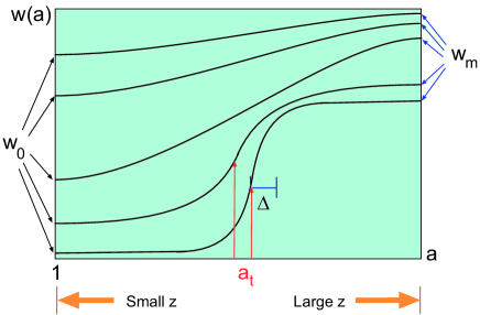
Figure 1: Schematic plot of the equation of state paratrisation Eq. (1).

Using this general prescription has a profound advantage in attempts to detect dark energy dynamics since, unlike simpler parametrisations based on only one or two variables, it can accurately describe both slowly and rapidly varying equation of states bck . Detecting dark energy dynamics and distinguishing it from a cosmological constant is difficult and is clear only when there are rapid, late-time, changes in $w$ CORAS3 , which then needs a formalism capable of describing such rapid transitions.

In order to compute the CMB power spectra, we use a modified version of the CMBfast Boltzmann solver ZALDA .

This is a non-trivial step in the case where $\Gamma$ changes rapidly (such as in our best-fit model!). In fact using a numerical method that is not able to track rapid transitions can lead to errors significantly larger than the error bars on the data, of order $5\%$, and consequently lead to completely wrong results. Our tests are described in detail in Appendix B and C.

Several degeneracies amongst the cosmological parameters prevent us from accurately constraining cosmological models using CMB data only. Specific features of the anisotropy power spectrum can provide information on particular combinations of the cosmological parameters. For instance the relative height of the Doppler peaks depends on the baryon density and the scalar spectral index. In order to break such degeneracies it is necessary to add external information. Since our goal is to constrain the properties of the dark energy, in a flat geometry the main limitation comes from the geometric degeneracy between $w_{0}$, the dark energy density $\Omega_{DE}$ and the Hubble parameter $h$. This degeneracy can be broken by assuming an HST prior on the value of $h$ FREEDMAN or/and combining the CMB with other data sets such as the matter power spectrum measurements from the 2dF galaxy survey Colless or the SN-Ia data. In our analysis we use the “gold” subset of the recent compilation of supernova data of RIESS04 in addition to the WMAP TT and TE spectra. An important point which we want to stress here is that CMB and SN data can be treated at a fundamental level without any prior assumption on the underlying cosmological model. For instance, this is the case for the matter power spectrum data from galaxy surveys which implicitely assumes a $\Lambda$CDM model when passing from redshift space to real space. For this reason we add the 2dFGRS large scale structure data only in order to check the stability of our results. We also remark that the use of secondary observables such as the age of the Universe, the size of the sound horizon at the decoupling, the clustering amplitude $\sigma_{8}$ (as quoted by the WMAP-team) or the growth factor of matter density perturbations should not be used without thought to infer constraints on the dark energy since their quoted value is usually derived by implicitly assuming a $\Lambda$CDM cosmology. This leads to biased results since these observables depend on the nature of the dark energy Doran01a ; Doran01b ; CORAS3 . In principle CMB constraints can be easily added by using the position of the Doppler peaks, which provide an estimate of the angular diameter distance to the last scattering surface. But it is a well known fact that pre-recombination effects can shift the peaks from their true geometrical position Doran01a .

The Integrated Sachs-Wolfe (ISW) effect also induces an additional shift in the position of the first peak, in a way that is strongly dependent on the evolution of the dark energy equation of state and is generally larger than in $\Lambda$CDM models CORAS3 . Therefore a consistent dark energy data analysis of the CMB indeed requires the computation of the CMB power spectrum (and TE cross-correlation).

Each of our models is then characterised by the dark energy parameters $\overline{W}_{DE}=(w_{0},w_{m},a_{t},\Delta)$ and the cosmological parameters $\overline{W}_{C}=(\Omega_{DE},\Omega_{b}h^{2},h,n_{S},\tau,A_{s})$, which are the dark energy density, the baryon density, the Hubble parameter, the scalar spectral index, the optical depth and the overall amplitude of the fluctuations respectively. We therefore end up with ten parameters which can be varied independently.

There is a remaining degeneracy in $n_{S}$, $\tau$ and $\Omega_{b}h^{2}$, which allows the models to reach unphysically high values of the baryon density and the reionisation optical depth. Following the WMAP analysis and in order to remain consistent with Kunz , we place a prior on the reionisation optical depth, $\tau\leq 0.3$. An alternative is to use a prior on $\Omega_{b}h^{2}$, which may be physically better motivated and does a better job of breaking the degeneracy – we plan to use this for future work and discuss the difference later on. We also limit ourselves to models with $w(z)\geq-1$, except where stated explicitly.

III Evaluation of the likelihood

A grid-based method would necessarily lead to a very coarse sampling, which is why we opted for a Markov-Chain Monte Carlo (MCMC) method to sample the likelihood surface. In addition this approach also allows easy marginalisation over parameters. We ran 16 to 32 independent chains on the UK national cosmology supercomputer (COSMOS). This approach has both the advantage that there was no need to parallelise the Boltzmann solver, and that we are better able to assess the convergence and exploration by comparing the different chains.

We take the total likelihood to be the product of the likelihoods of each data set (CMB, SN-Ia and LSS), or by defining $\chi^{2}_{\rm eff}\equiv-2\log\mathcal{L}$,

$$\chi^{2}_{\rm tot}=\chi^{2}_{\rm WMAP}+\chi^{2}_{\rm SN1a}(+\chi^{2}_{\rm 2dF}),$$ (2)

where the LSS contribution is added only in section IV.4. We evaluate the WMAP likelihood using the code of the WMAP science team VERDE , and we have checked that our SN-Ia likelihood results are consistent with ones of Riess et al RIESS04 . We treat the luminosity $\cal{M}$ as a nuisance parameter over which we marginalise analytically. This automatically also marginalises over the Hubble constant $H_{0}$, so that the supernova data does not depend directly on it. For the 2dF results we use the formalism and data of Tegmark tegmark_2df .

The convergence and sampling behaviour of the chains in a high-dimensional space is far from trivial. Correlations in several dimensions are a particular issue as they lead to a high rejection rate. To improve the acceptance rate, we estimate in a first step the covariance matrix and then use rotated parameters which are linearly independent (i.e. lead to a diagonal covariance matrix with variances $\sigma(p_{i})^{2}$ on the diagonal). We set the proposal width of parameter $p_{i}$ ($i=1,..,N$) to $2.3\sigma(p_{i})/\sqrt{N}$ as advocated in gilks ; dunkley , which we found to work very well. We also evaluate the rejection rate every 100 steps and adjust the width dynamically, but normally this is not necessary once the covariance matrix is used.

The result of a MCMC is a “cloud” of samples in each chain with a density proportional to the local value of the likelihood. In general we are not content with a N-dimensional description of the likelihood, but would prefer lower dimensional constraints. The generally accepted way to project the likelihood onto fewer dimensions is through marginalising. This means that we integrate the likelihood over the parameters which we want to hide,

$$\mathcal{L}(p_{1},\ldots,p_{i-1},p_{i+1},\ldots,p_{n}) \propto$$

$$\int dp_{i}\mathcal{L}(p_{1},\ldots,p_{i-1},p_{i},p_{i+1},\ldots,p_{n})$$ (3)

This requires a measure $\mu=dp$ on the parameter space. In many cases, there is some physical motivation for the choice of the measure. Alternatively, it may be that the for all reasonable choices, the measure does not vary strongly across the range of interest. As an example, we could use either $\Omega_{b}$ or $\Omega_{b}h^{2}$ as a fundamental parameter. But since both $H_{0}$ and $\Omega_{b}h^{2}$ are quite well constrained, the result will not change appreciably if we use the one or the other. In this case, it does not matter which one we use. If neither is true then the result can depend strongly on the choice of this measure.

In the MCMC case, the choice of measure is implicit in the choice of parameters if one follows the usual rule that the marginalisation is done by summing up the samples. To illustrate this, let us assume that the likelihood does not depend upon a given parameter $0.1\leq p\leq 10$. In this case, the marginalisation over this parameter is just the volume of the parameter space, since all values are equally likely. The resulting likelihood will be flat, independent of the choice of parametrisation. Using $p$ as our fundamental parameter, we find that roughly half the points will be in $p<5$ and half in $p>5$. On the other hand, using $\log p$ we will find that half the points are in $p<1$, and half in $p>1$. The result depends in this case strongly on the choice of parametrisation. We would like to add here that a linear transformation of the parameters does not change the measure, as long as the boundaries of the integration are also adjusted. This is normally the case, since the integration volume is usually given by the region where $\mathcal{L}\neq 0$. An example of such a transformation is the use of a covariance matrix to render the parameters linearly independent.

A different way to think about this specific problem, is by looking at the choice of measure as a prior. Choosing for a parameter $p$ the measure $dp$ (i.e. sample it equally in $p$) is the same as imposing a flat prior, $P(p)=1$. Instead, sampling the parameter in $\log(p)$, corresponding to a measure $dp/p$, corresponds to a flat prior in $\log(p)$ or $P(p)=1/p$ when sampling evenly in $p$ tegmark_sdss .

In order to test our dependence on the choice of parametrisation, we ran chains for different choices, namely $(a_{t},\Delta)$, $(\log(a_{t}),\Delta)$ and $(\log(a_{t}),\log(\Delta))$. In the next section we will discuss which of the results depend on this choice.

A second issue which is often neglected is that the likelihood which we deal with here is by no means close to Gaussian in some of the variables. The structure of the minima can thus be arbitrarily complicated. It is therefore important to specifically search for the global minimum, which can of course be rather difficult in many dimensions.

As a final remark before discussing the results, we would like to point out that caution is necessary when interpreting the results. One sigma limits are not sufficient to rule out anything – the true model is indeed expected to lie about one sigma away from the expectation value! Even two sigma or 95% (the limits which we usually quote) are not sufficient. We present here limits and constraints on well over 20 different variables, and so we again expect at least one to lie in the excluded region. Even worse, Gaussian statistics are well known to underestimate the tails of “real world” distributions, so that outliers are far more common than naively expected. In many fields, e.g. particle physics, a 5 sigma limit is being used to claim an actual detection. Although our data is not yet of sufficient quality to impose such stringent limits, we should bear this in mind. So we should as an example only consider regions ruled out in the 1-dimensional likelihood plots if the likelihood has (visually) fallen to zero.

IV Results

In this section we discuss different aspects of our results. We start by taking a look at the best-fit models and at the goodness-of-fit of both quintessence and $\Lambda$CDM models. Then we show that the introduction of a time-varying equation of state for the dark energy component does not significantly alter the constraints on the basic cosmological parameters. This allows us to discuss constraints on the time evolution of the quintessence equation of state. In section IV.4 we use large-scale structure data instead of the supernova data to break the geometric degeneracy. We also check if the combination of both data sets improves the constraints. Finally, we discuss limits on toy “phantom energy” models where we allow $w<-1$.

IV.1 The goodness of fit

Our global best fit QCDM model is characterized by the following dark energy parameters: $w_{0}=-1.00$, $w_{m}=-0.13$, $a_{t}=0.48$ and $\Delta=0.06$, which correspond to a fast transition in the equation of state at redshift of $1$. The total $\chi^{2}$ of this model is $1602.9$, while the best-fit $\Lambda$CDM model has $\chi^{2}=1605.8$. However, the total number of degrees of freedom is 1514, so that all our fits are rather bad. This is mainly due to the WMAP data (see the discussion in SPERGEL ). In table 1 we report the corresponding $\chi^{2}$ values for the CMB and SN data and best fit values of the standard cosmological parameters for these two models. Notice that the QCDM model provides the best fit to both the CMB and SN data.

Model	$\chi^{2}_{CMB}$	$\chi^{2}_{SN}$	$\chi^{2}_{tot}$	$w_{0}$	$\Omega_{DE}$	$H_{0}$	$\Omega_{b}h^{2}$	$n_{s}$	$\tau$
$\Lambda$CDM	$1428.7$	$177.1$	$1605.8$	$-1.0$	$0.69$	$69$	$0.023$	$0.97$	$0.11$
QCDM	$1426.1$	$176.8$	$1602.9$	$-1.0$	$0.71$	$67$	$0.026$	$1.09$	$0.29$

Table 1: $\chi^{2}$ and best fit values of the cosmological parameters for $\Lambda$CDM and QCDM models.

It is intriguing that such a model has a time evolving equation of state $w(z)$ similar to that reconstructed from the best fit to the SN data in Alam ; Peri ; Cooray . In figure 2 we plot the temperature anisotropy power spectrum for these two models. It is remarkable how perfectly the two completely different models agree at intermediate $\ell$, demonstrating the power of the WMAP CMB data. At low multipoles the additional freedom of the QCDM models allows a slightly better fit. In fact due to a different distribution of the ISW, these QCDM best fit models have less power at low multipoles than the $\Lambda$CDM one. However we want to remark that this part of the CMB spectrum is most likely affected by galactic contamination effects Slosar and without a more accurate investigation we should not place too much emphasis on this suppression of power. It is worth noticing that the difference in the best-fit cosmological parameters between QCDM and $\Lambda$CDM will lead to different TT power spectra at higher multipoles, $l>700$. This suggest that an accurate detection of the third peak may increase the statistical weight in favour or against the QCDM model.

Figure 2: CMB power spectrum for the QCDM (red solid line) and $\Lambda$CDM (blue dashed line) best fit models.

The fact that the $\chi^{2}$ improves by $3$ through the addition of the three new dark energy parameters, is to be expected. Nevertheless we see that some quintessence models provide a better fit to the data than standard $\Lambda$CDM , as opposed to analyses which assume that $w$ is constant. As we will discuss later, the limits on the time evolution of the dark energy equation of state are still compatible with a number of proposed scalar field scenarios.

Studying the distribution of the $\chi^{2}$ values in the MCMC chains for the $\Lambda$CDM models, we find that $\Delta\chi^{2}=6.4$ for the models at $1\sigma$ (68.3% CL) and $\Delta\chi^{2}=11.8$ at $2\sigma$ (95.4% CL). In the Gaussian case, this corresponds to about $5.5$ independent degrees of freedom, slightly less than the number of cosmological parameters used ($6$).

For the quintessence models we find $\Delta\chi^{2}=9.9$ for $1\sigma$ and $\Delta\chi^{2}=15.5$ for $2\sigma$. Assuming Gaussian errors, this would mean that we are dealing with about $8$ independent degrees of freedom, many less than the $6$ cosmological and $4$ dark energy parameters used in the analysis. We conclude that we are unable to constrain all the additional parameters.

Is the improved $\chi^{2}$ of the best fit QCDM models a positive evidence for the additional dark energy parameters? The answer to this question requires an estimation of the information criteria associated with the model andrew_aic . In general adding more parameters tends to improve the fit to data, however one should reward thoes models that can produce the same goodness-of-fit with fewer parameters. This can be achieved through the Akaike information criterion (AIC Akaike ) and Bayesian information criterion (BIC Bic ), respectively defined as

$$AIC=-2\ln{\mathcal{L}}+2k,$$ (4)

and

$$BIC=-2\ln{\mathcal{L}}+k\ln{N},$$ (5)

where $\mathcal{L}$ is the maximum likelihood, $k$ is the number of parameters of the model and $N$ is the number of datapoints. The $\Lambda$CDM models have an AIC of $1617.8$, while the QCDM models of $1622.9$. Based on this difference of $5$ we conclude that four parameter dark energy models are not necessarily favoured. The BIC disfavours the new parameters even more strongly. The information criteria therefore suggest that current data provide no positive evidence that the dark energy is anything more complex than a cosmological constant. This is not surprising, but should not be used as a reason to stop searching for ways of detecting evidence of evolution. The rewards from finding such evidence would be huge.

IV.2 Constraints on cosmological parameters

The class of quintessence models could a priori contain new, severe degeneracies which change completely the preferred values of the cosmological parameters. If this were the case, then all the standard results of the WMAP analysis SPERGEL would only be valid in the context of a $\Lambda$CDM model. We have found this not to be the case. The new dark energy parameters are degenerate amongst themselves but do not introduce any new degeneracy with the other cosmological parameters. This can be seen in figure 3 where quintessence model results are compared with those obtained for $\Lambda$CDM models only. Unless specifically stated, the quoted results have been obtained using a linear parametrisation of $a_{t}$ and a logarithmic one of $\Delta$ in the MCMC. This maximises the weight of models with a late rapid transition, other parametrisations lead to an even slightly better agreement between $\Lambda$CDM and QCDM.

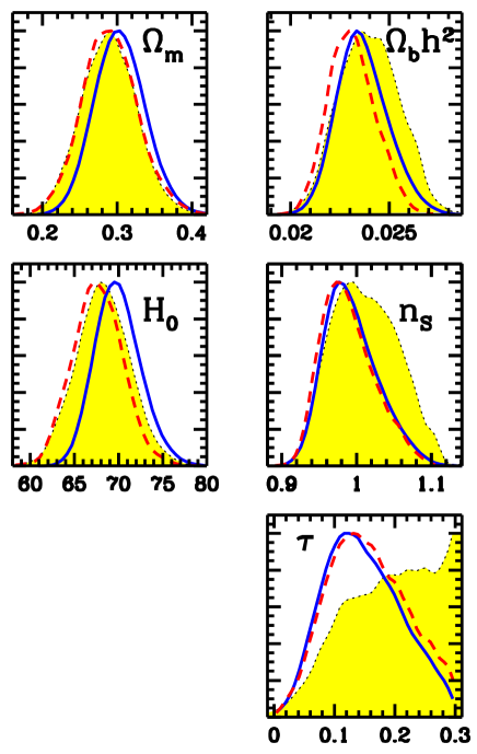
Figure 3: Marginalized likelihoods for the various cosmological parameters in the $\Lambda$CDM scenario (blue solid curve) and including the QCDM models (yellow shaded region). Also shown are QCDM models with a prior on the baryon energy density $\Omega_{b}h^{2}=0.0216\pm 0.002$ (red dashed line). The results agree very well in all cases.

We notice that all parameters, with the possible exception of the reionisation optical depth $\tau$, are well determined in both cases. Also, their values are very similar and cannot be distinguished even at one standard deviation. Table 2 lists the best fit values of the cosmological parameters for the $\Lambda$CDM and the dark energy models. The constraint on $h$ is consistent with the HST measurement FREEDMAN , while the amount of clustering matter $\Omega_{m}$ is in agreement with large scale structure estimates perci ; allen . The physical baryon density is consistent with the Big-Bang Nucleosynthesis expectations BBN . This provides an important cross-check that all viable models have to pass. The background universe is therefore largely independent of the details of the dark energy.

Parameter	$\Lambda$CDM	QCDM
$\Omega_{m}$	$0.30\pm 0.03$	$0.29\pm 0.04$
$\Omega_{b}h^{2}$	$0.0237\pm 0.0013$	$0.0240\pm 0.0015$
$H_{0}$	$70\pm 3$	$68\pm 3$
$n_{s}$	$0.99\pm 0.04$	$1.01\pm 0.04$
$\tau$	$0.15\pm 0.06$	$0.19\pm 0.07$

Table 2: Mean and (formal) standard deviations for the cosmological parameters. The $\Lambda$CDM values agree with published analyses. The QCDM values are always consistent within one standard deviation, showing that quintessence does not significantly impact “precision cosmology”.

We find nonetheless some differences, but they can be explained quite easily. Firstly, these are the marginalised likelihoods. The remaining degeneracy in $\Omega_{m}$, $H_{0}$ and $w_{0}$ is therefore translated into a slight shift to lower values in both $\Omega_{m}$ and $H_{0}$. The degeneracy between the physical baryon density, $\Omega_{b}h^{2}$, and the scalar spectral index, $n_{S}$, becomes slightly worse (see figure 4), leading to somewhat longer tails in their likelihood distributions. This is a consequence of the larger Integrated Sachs-Wolfe (ISW) effect produced in time dependent dark energy models with the respect to the $\Lambda$CDM case CORAS3 . In fact the ISW boosts power on the large angular scales of the CMB, therefore less power of the primordial fluctuation power spectrum at small wavenumber $k$ is required to match the data. Consequently slightly blue shifted spectral index values are preferred. The same effect is also responsible for the spread of the likelihood distribution of the reionisation optical depth through the degeneracy between $n_{s}$ and $\tau$. For larger values of $n_{s}$ the excess of power at the low multipoles of the TE spectrum requires larger values of the optical depth (see figure 5). Since the reionisation suppresses the contribution at high $\ell$ with a factor of $e^{-2\tau}$ a better determination of the CMB peak structure as well as better polarisation data will help to break this degeneracy. We hope that the latter will be available shortly, when WMAP releases the two-year data.

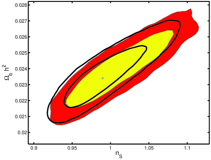
Figure 4: The degeneracy between the scalar spectral index, $n_{S}$, and the physical baryon density $\Omega_{b}h^{2}$. The filled contour are the 1 and 2 $\sigma$ limits of the quintessence models, while the black solid contours are those of the $\Lambda$CDM models.

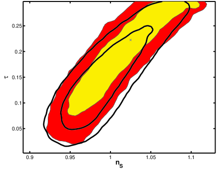
Figure 5: The degeneracy between the scalar spectral index, $n_{S}$, and the optical depth $\tau$. The filled contour are the 1 and 2 $\sigma$ limits of the quintessence models. The black lines show the corresponding limits for the $\Lambda$CDM case.

Figure 3 shows also the effect of introducing a prior on $\Omega_{b}h^{2}$, namely $\Omega_{b}h^{2}=0.0216\pm 0.002$. As we can see, the prior only affects the cosmological parameters $\tau$, $n_{S}$ and $\Omega_{b}h^{2}$ and removes some of their high values. None of the dark energy parameters are affected (see figure 6). We should note that all cases use a top-hat prior $\tau<0.3$.

IV.3 Constraints on the dark energy parameters

As we have seen in the previous section, the additional parameters which describe the dark energy do not introduce any new degeneracies with the standard cosmological parameters. However we expect the dark energy parameter space to have an internal degeneracy. For instance $w_{0}$ and $w_{m}$ both act on physical observables as an equation of state parameter. Therefore slowly varying models with $w_{m}\approx w_{0}$ may look indistinguishable from models with the same value of $w_{0}$ and a rapid transition at very early time from whatever value of $w_{m}$. As anticipated in Section IV.1, the consequence of such degeneracy is that we can strongly constrain only one of the dark energy parameters, which turns out to be $w_{0}$. In particular, the one-dimensional marginalized likelihood gives $w_{0}<-0.80$ at $2\sigma$, which is consistent with the upper limits quoted in other time dependent dark energy analyses LUCA ; DORAN ; WANG . Of course what this really implies is that the equation of state at a redshift of order z=0.1 is being constrained. We can not say anything about its true value today, but in what follows we use $w_{0}$ with this caveat in mind. The same applies when we take the limit of $z\to 0$ in the relevant figures.

The other dark energy parameters are weakly constrained. In particular, as expected from the arguments discussed in Section III, we find that the inferred confidence intervals may depend on the parametrisation of $a_{t}$ and $\Delta$ used in the MCMC. For the standard case, we find $w_{m}<-0.08$ at $2\sigma$, on the other hand $a_{t}$ and $\Delta$ remain unconstrained. We refer to Kunz for a discussion on breaking such a degeneracy with an estimate of the value of $\sigma_{8}$ from large scale structure.

A parametrisation in $\log(a_{t})$ would place more emphasis on early transitions, so that the effective redshift where $w_{m}$ is evaluated is moved to higher values. In this case the limits on $w_{m}$ become even weaker, and we conclude that $w_{m}$ as a parameter is difficult to interpret. On the other hand, the limits on $w(z)$ as a function of redshift are less dependent of the parametrisation of $a_{t}$, as we derive them at all redshifts separately. We therefore advocate these limits, as plotted in figure 7, as a better illustration of the constraints on dark energy models.

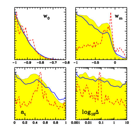
Figure 6: Likelihoods for the dark energy parameters in the QCDM models without prior on $\Omega_{b}h^{2}$ (yellow shaded area) and with the prior (solid blue line). The prior does not affect the dark energy parameters significantly. We also show the relative goodness of fit of the best model in each bin (red dashed lines).

These limits, derived with the Markov-Chain approach, rest solely on the local density of the accepted models. If the assumption of Gaussian errors holds approximately, then we can derive the same limits using the actual likelihood values instead. In this case, and considering a single variable, models with $\Delta\chi^{2}<4$ occur 95.4% of the time. We find that models with $w_{0}>-0.8$ have $\Delta\chi^{2}>4$, consistent with the limits from the Markov Chain. In order to put limits on the equation of state as a function of redshift, we proceed as follows: we compute $w(z)$ for each model and then take either the $95\%$ confidence region over all models in the chain (shaded area in figure 7) or compute the highest $w(z)$ for models with $\chi^{2}<\chi^{2}_{\rm min}+4$ (dashed line).

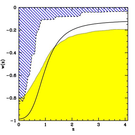
Figure 7: $2\sigma$ confidence region on $w(z)$ derived by taking the 95% models with lowest $w(z)$ from our main chain (yellow shaded area) and the “exclusion zone” where all models have $\Delta\chi^{2}>4$ from the best-fit model in our main chain (blue hatched area). We also show the $w(z)$ of the best-fit model (black solid line). $\Lambda$CDM is acceptable at $2\sigma$.

The shaded area is a priori the proper marginalised result, representing the $95\%$ limits on $w(z)$. However it is worth remarking that this constraint may suffer from a potential problem with the choice of the measure that we introduce to integrate the marginalised parameters over (see discussion in section III). On the other hand the dashed line relies only on the goodness of fit, and can be interpreted as an exclusion limit. In other words models with a $w(z)$ that enter the hatched area are a “bad” fit to the data. This does not include any information about how likely these models are, given the variation in the other parameters. Our interpretation of this is as follows: if we want to judge if a single, specific model is ruled out or not, then we should be using the dashed line as an upper limit for $w(z)$. If we are more interested in what we would expect as the value of $w(z)$, given our additional knowledge about the other variables, then we should look at the shaded region as providing a limit on the equation of state parameter. As we can see in figure 7, models with $w_{m}\geq 0$ at $z>1$ and with a fast transition occurring at $z\lesssim 1$ are a bad fit to the data, being beyond the dashed blue line. Physically this is because models where the transition from $w_{m}$ to $w_{0}$ occurs at redshifts $z<10$ with $w_{m}>-0.1$ give rise to a non-negligible dark energy energy contribution at decoupling, which is strongly constrained by CMB data. However, models with $w_{0}<-0.8$ and $w_{m}>-0.1$ for which the transition occurs at redshift $z>10$ are consistent with the data as their early energy contribution is negligible. As mentioned earlier, the apparent exclusion of these models based on the likelihood for $w_{m}$ in figure 6 is an artifact of our parametrisation of $a_{t}$. This can also be seen by noticing that the maximised results (dashed curve) does not fall to zero for $w_{m}>0$, indicating that there are acceptable models in this part of the parameter space. However these models will be indistinguishable from a pure $\Lambda$CDM scenario and are thus not very interesting when we try to rule out one from the other.

The limits on $w(z)$ can be reinterpreted as constraints on the evolution of the dark energy density (see figure 8). Models with $\Omega_{DE}(z)$ above the dashed line are ruled out, thus limiting the amount of dark energy available during matter domination to be $\Omega_{DE}(z)<0.1$ (see also DORAN ; Doran ).

These results undoubtedly have an effect for quintessence model building, and we will be investigating this aspect in a future paper.

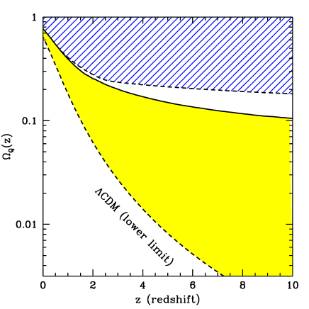
Figure 8: Limits on $\Omega_{DE}(z)$ corresponding to those on $w(z)$ in figure 7.

For now though we restrict ourselves to a few general remarks. The limits on $w(z)$ previously obtained allow us to constrain a large class of quintessence models. For instance the exclusion plot in figure 7 suggests that models with a perfect tracking behavior, for which $w=0$ during the matter era up to $z\leq 4$, and with a late time fast transition, are disfavoured by the data. As we have seen before, this is because $\Omega_{Q}$ must be negligible at early times. This class of models, for some particular choice of the parameters of the scalar field potential, include the two exponential potential NELSON and the Albrecht-Skordis model ALBRECHT . Of course, if they leave their tracking behaviour before then, the constraint is weakened. These models satisfy the constraints only if the slope of the scalar field potential, where the quintessence is initially rolling down, is very steep and then followed by a nearly flat region such that the equation of state $\approx-1$ at the present time. On the other hand models with a non-perfect tracking behavior and a slowly varying equation of state with $w_{0}<-0.8$ are consistent with the data. This is the case of quintessence models with an inverse power law potential Ratra , supergravity inspired potentials such as the one proposed in BRAX or off-tracking quintessence models, such as those studied in Axel ; Kneller . Models of late time transition PL which show features of our best fit model can also be consistent with the data.

IV.4 Adding large scale structure

One important question is whether the supernova data contains any severe systematic effects that may strongly bias our results. To test for this possibility, we replace the supernova data by the 2dF galaxy redshift survey power spectrum from ref. tegmark_2df . The bias is added as a new, free parameter. This means that only the form of $P(k)$ is constrained, not its amplitude. The solid lines in figures 9 and 10 show the resulting likelihoods of the cosmological and the dark energy parameters respectively. Comparing them to the CMB+SN-Ia results (shaded yellow regions), we find that the results are consistent, but that the supernovae allow us to place stronger constraints on $\Omega_{m}$, $H_{0}$ and $w_{0}$ when combined with the CMB. There is no evidence for any systematic problems in the SN-Ia data set.

Additionally, we can use the combination of all three data sets. In BRUCE we found that the large scale structure (LSS) does not add any strong constraints, beyond those found with CMB+SN-Ia data, as long as no constraints on the bias parameter are imposed. As the dashed curve in figures 9 and 10 shows, this is still the case, and the bias parameter is strongly correlated with the clustering strength, $\sigma_{8}$. The constraints on the bias found in POPE do not apply to our analysis, since they were obtained by combining the SDSS 3D matter power spectrum with the WMAP results on $\sigma_{8}$ which are correct only for $\Lambda$CDM cosmologies.

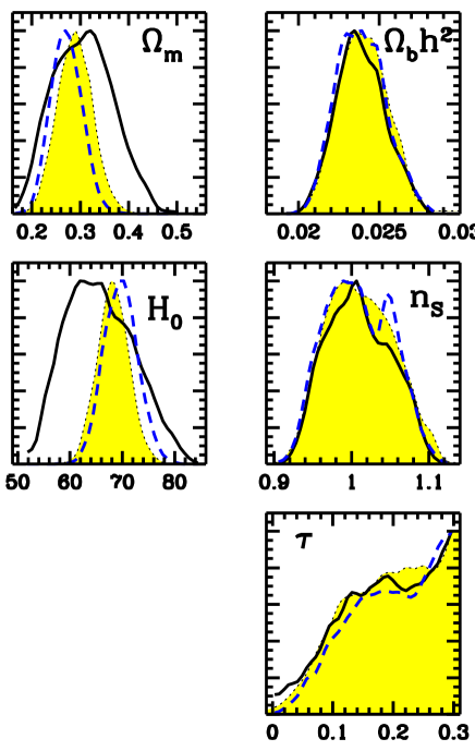
Figure 9: Constraints on the cosmological parameters when adding the 2dFGRS data to CMB and SN-Ia data (blue dashed line) and when only using CMB+2dFGRS (black solid line), compared to the CMB+SN-Ia case (yellow shaded region).

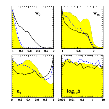
Figure 10: Constraints on the dark energy parameters when adding the 2dFGRS data to CMB and SN-Ia data (blue dashed line) and when only using CMB+2dFGRS (black solid line), compared to the CMB+SN-Ia case (yellow shaded region).

For standard quintessence models one can thus either use supernovae or large scale structure data, with the supernova data giving the stronger constraints. The situation changes if additional parameters need to be constrained, e.g. non-zero neutrino masses. In this case it is crucial to have very good clustering data on small scales where the neutrinos impose a distinct signal on $P(k)$.

IV.5 Phantom energy models

Several authors have suggested that dark energy models with a super-negative equation of state, for which $w<-1$, can provide a better fit to the CMB and the SN-Ia data CAL ; MORT ; TROD ; KamCald ; Jochen . On the other hand all these analyses are biased in favour of phantom dark energy models since they use a constant equation of state parameter MAOR ; VIREY . In this scenario the dark energy violates the weak energy condition (WEC) which leads to a number of problems CAR . For this reason we feel that these models are disfavoured on theoretical grounds. Nevertheless it remains an interesting question whether they are compatible with the current cosmological observations? Constraining time dependent phantom energy models allows us the opportunity to test these models against the observational data without the bias induced by assuming a constant equation of state parameter. However the main problem for this class of models is the existence of tachyon instabilities which lead to an exponential growth of phantom energy perturbations on small scales. In addition our formalism does not allow us to follow the evolution of the dark energy perturbations for phantom models which cross the $w=-1$ value (see discussion in Appendix B). On the other hand we can account for the perturbations in models which violate the weak energy condition at all times.

In order to be self-consistent we therefore extend our analysis to two different classes of dark energy models, those which always satisfy/violate the WEC and those which cross the WEC boundary value $w=-1$. The latter are assumed to be homogeneous and consequently our analysis for these class of models accounts only for the effects they produce on the background expansion. Although this is not physical, we are unaware of a unique prescription for handling these cases. We therefore suggest that the reader sees this section more as a speculative treatment. It is interesting to note that in these “toy” phantom models, the allowed values of the cosmological parameters do not change very much, in that they lie somewhere between the $\Lambda$CDM and the QCDM case (see Fig. 11).

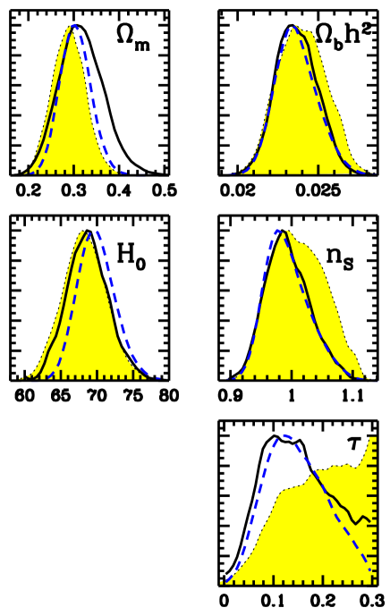
Figure 11: Constraints on the cosmological parameters for all phantom models (solid lines) and those that respect the weak energy condition ($w\geq 1$) (shaded), compared to the $\Lambda$CDM models (dashed).

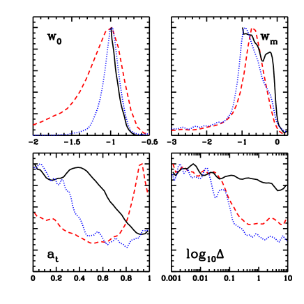
Figure 12: Constraints on the dark energy parameters for all phantom models (red dashed lines) and those that respect the weak energy condition ($w\geq-1$) (solid black line). The dotted line is from models that do not cross $w=-1$.

The models which cross $w=-1$ provide a slightly improved best-fit. In particular we find a best-fit model with $\chi^{2}=1601$. It has $w_{0}=-2.0$ and $w_{m}=-0.7$, i.e. the equation of state crosses over that of the cosmological constant, $p=-\rho$. This behaviour is most likely driven by the supernova data, as we find a similar result if we only use this data set bck .

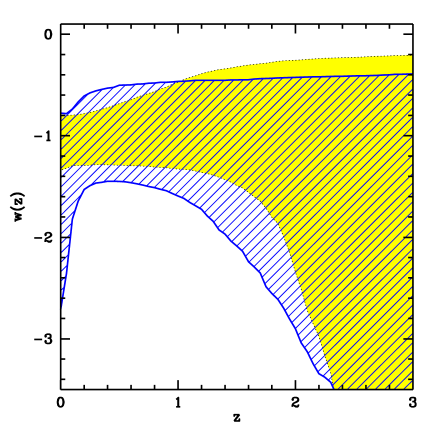
Figure 13: Constraints on the dark energy equation of state parameter $w(z)$. The shaded area corresponds to models which do not cross $w=-1$ and for which perturbations are taken into account, while the hatched area corresponds to all models, including those crossing $w=-1$, but without perturbations.

For the standard parametrisation of $a_{t}$ and $\Delta$, the median for $w_{0}$ is $-1.1$ and for $w_{m}$ is $-0.8$. The 95% confidence intervals are $-2.7<w_{0}<-0.77$ and $-8.3<w_{m}<-0.19$. For the models that do not cross $w=-1$, but always remain either with $w<-1$ or $w\geq-1$, the results give the median for $w_{0}$ to be $-1.0$ and for $w_{m}$ to be $-0.97$. The overall best-fit model is the same as for the standard QCDM models, but as the above median values show there are about the same number of accepted models on both sides of the divide.

Thus there is no evidence for any deviation from $\Lambda$CDM in this extended framework.

The parameter which does show some change is the clustering amplitude, $\sigma_{8}$, which lies now in the 95% confidence interval $0.66<\sigma_{8}<1.24$ as opposed to the dark energy models satisfying the weak energy condition $w\geq-1$ for which $0.53<\sigma_{8}<1.07$.

The limits on $w(z)$ are shown in figure 13. The shaded regions correspond to all models which do not cross $w=-1$ and for which perturbations are included, while the hatched area corresponds to all models which cross $w=-1$.

V conclusions and outlook

In this paper we have made the first attempt to constrain dynamical models of dark energy by combining CMB, 2dFGRS and type-Ia supernova data. On the positive side, we find that by allowing the dark energy equation of state to vary as a function of time, we do not introduce any strong degeneracies that would adversely affect the standard cosmological parameter estimation, apart from perhaps a mild degeneracy between the reionisation optical depth, $\tau$ and the redshift of the commencement of acceleration. Its effect is to alter the ISW contribution to large angles and hence, after COBE normalisation uniformly alters the heights of the peaks BRUCE . Breaking this degeneracy by some means will significantly enhance our ability to constrain dark energy dynamics. This might be done through a number of routes: other astrophysical constraints on $\tau$; by probing the redshift of acceleration using ISW-LSS correlations; by measuring the non-Gaussianity of CMB from weak lensing induced by structure formation Fabio or by beating cosmic variance using cluster polarisation at high redshift variance .

The remaining cosmic parameters are only mildly affected by the new freedom given to dark energy and are similar to their $\Lambda$CDM counterparts. On the down side, with regard to the dark energy parameters, the currently available data set means that only the present value of the equation of state $w_{0}$ is well constrained. We find $w_{0}<-0.8$ at 95% confidence level. By studying the behaviour of $w(z)$, we conclude that the constraints become weak for any redshifts larger than about unity.

However, there are some clear results that emerge. For example in the large class of Quintessence models that have periods of perfect tracking behaviour, i.e. $w=0$ during the matter dominated era, only those which track for during the period $z\stackrel{{\scriptstyle>}}{{\sim}}5$ are acceptable. Quintessence models with a very late departure from tracking, or any dark energy models with a late transition from a high value of $w$, are disfavoured as a consequence of the fact that early contributions of dark energy are constrained to be negligible.

We have also found a point of practical importance in the hunt for dark energy dynamics. Since only rapidly varying models at low redshift have a distinct signature as opposed to $\Lambda$CDM CORAS3 including such models in ones likelihood analysis is very important, otherwise the results will be biased towards no detection of dynamics. However these rapidly varying models are the most susceptible to numerical errors, which we have found can be as large as $5\%$. We therefore have used a code specially adapted to handle these ”kink” cases, and this is described in Appendix C.

We have also studied toy models for which $w<-1$ is possible. In this case the perturbations are generically unstable, and so we turned them off for any model which enters $w<-1$ at any point. In this case models that have $w$ slightly larger than $-1$ at early times and show a rapid, late transition to a super-negative equation of state, $w\stackrel{{\scriptstyle<}}{{\sim}}-2$, are slightly, but not significantly, preferred. In a slightly more physical model where $w=-1$ cannot be crossed, allowing us to compute the perturbations, we find no preference for these “phantom” models.

Overall, we conclude that dynamical models of dark energy are by no means ruled out and provide a slightly better fit to current data than $\Lambda$CDM . The latter is still perfectly acceptable and, given its simplicity, seems in many ways the preferred model at the current time. Whether observations and theoretical prejudice maintain this conclusio over the coming years will have a profound impact on our understanding of fundamental physics.

Appendix A Parametrisation of the models

A simple way of describing a dark energy component is to consider a constant equation of state $w$. However such an approach suffers from a number of drawbacks. In fact assuming $w$ to be constant introduces a bias in the analysis of cosmological distance measurements with the consequence that large negative values of $w$ are favoured if the dark energy is time dependent MAOR ; VIREY . The effect of this bias has to be carefully taken into account particularly when models of phantom energy CAL ; CAR , for which $w<-1$, are constrained. A possible way to address this issue is to constrain a time dependent parametrisation of $w(z)$. In fact the time dependence of the dark energy equation of state completely specifies the evolution of the dark energy density through the continuity equation. Several formula have been proposed in the literature GERKE ; WELLA ; LINDER ; PADMA all with limited applicability. They are typically based on Taylor expansions in some variable (e.g. $z$, $\log(1+z)$ or $1-a$).

However, tracking quintessence models exhibit the important property that before the universe begins to accelerate the dark energy has an equation of state which mimics that of the dominant energy component. Today of course $w<-1/3$, so there must be a transition between the value at high redshifts and that at the present time at some critical redshift, $z_{t}$, or equivalently scale factor, $a_{t}=1/(1+z_{t})$, with a thickness determined by a parameter $\Delta$. In fact, this physically motivated parametrisation bears a striking resemblance to the $\tanh(z)$ kink soliton solution in spirit.

To compare various proposals we write it as:

$$w(a)=w_{0}+(w_{m}-w_{0})\Gamma(a,a_{t},\Delta);$$ (6)

where $\Gamma$ determines precisely how the transition from $w=w_{m}$ to $w=w_{0}$ occurs. Two proposals for $\Gamma$ have been made in the literature. The original oneBRUCE ; CONDENSATION uses $z$ instead of $a$:

$$\Gamma(z,z_{t},\Delta)=\frac{-1}{1+e^{\frac{z-z_{t}}{\Delta}}}$$ (7)

while a different proposal (and the one that we use here) was made in CORAS2 , namely:

$$\Gamma(a,a_{t},\Delta)=\frac{1+e^{\frac{a_{t}}{\Delta}}}{1+e^{-\frac{a-a_{t}}{\Delta}}}\times\frac{1-e^{-\frac{a-1}{\Delta}}}{1-e^{\frac{1}{\Delta}}}$$ (8)

The latter form has the advantage of being more stable numerically (since $a$ is bounded in the interval $[0,1]$ while redshifts up to $z=10^{4}$ must be considered in the first form) and satisfies $w(a=1)=w_{0}$ whereas the same is only true for sufficiently rapid transitions in eq. (7). Because of this we use the latter form (8) in this paper.

Importantly, this form can also be extended CORAS2 to allow for a different value of $w$ during radiation domination so that it can represent tracking models faithfully at all redshifts in terms of five physical parameters: the value of the equation of state today $w_{0}$, during the matter era $w_{m}$ and during the radiation era $w_{r}$, while the time dependence is specified by the value of the scale factor $a_{t}$ where the equation of state changes from $w_{m}$ to $w_{0}$ and the width of the transition $\Delta$. Since Big-Bang Nucleosynthesis bounds limit the amount of dark energy to be negligible during the radiation dominated era BEANMEL the extra freedom is not particularly important and we further reduce our parameter space by setting $w_{r}=w_{m}$ yielding the transition function (8).

Written out fully then, the equation of state we use in this paper is Eq. (4) of ref. CORAS2 :

$$w(a)=w_{0}+(w_{m}-w_{0})\times\frac{1+e^{\frac{a_{t}}{\Delta}}}{1+e^{-\frac{a-a_{t}}{\Delta}}}\times\frac{1-e^{-\frac{a-1}{\Delta}}}{1-e^{\frac{1}{\Delta}}}.$$ (9)

The dark energy parameters specified by the vector $\overline{W}_{DE}=(w_{0},w_{m},a_{t},\Delta)$ with the parametrisation given by Eq. (9) can account for most of the dark energy models proposed in the literature (see CORAS2 for a detailed discussion). For instance, models characterized by a slowly varying equation of state, such as supergravity inspired models BRAX , correspond to a region of our parameter space for which $0<a_{t}/\Delta<1$, while models with a rapid variation of $w(a)$, such as the two exponential potential NELSON or the Albrecht-Skordis model ALBRECHT , correspond to $a_{t}/\Delta>1$. Models with a simple constant equation of state are given by $w_{0}=w_{m}$. We can account also for the so called phantom energy models for which $w_{0},w_{m}<-1$. The cosmological constant model corresponds to the following cases: $w_{0}=w_{m}=-1$ or $w_{0}=-1$ and $a_{t}\lesssim 0.1$ with $a_{t}/\Delta>1$.

Appendix B Cosmological evolution of scalar fields

The cosmological evolution of minimally coupled quintessence field Q is described by the Klein-Gordon equation,

$$Q^{\prime\prime}+2\frac{a^{\prime}}{a}Q^{\prime}+a^{2}\frac{dV}{dQ}=0,$$ (10)

the prime denotes derivatives with the respect to conformal time, $V(Q)$ being the scalar field potential and

$$\left(\frac{a^{\prime}}{a}\right)^{2}=\frac{8\pi G}{3}\left[\rho_{m}+\rho_{r}+\frac{{Q^{\prime}}^{2}}{2a^{2}}+V(Q)\right],$$ (11)

where $\rho_{m}$ and $\rho_{r}$ are the matter and radiation energy density respectively. The equation of motion for the quintessence fluctuations at the scale $k$ in the synchronous gauge is given by

$$\delta Q^{\prime\prime}+2\frac{a^{\prime}}{a}\delta Q^{\prime}+(a^{2}\frac{d^{2}V}{dQ^{2}}+k^{2})\delta Q=-\frac{1}{2}Q^{\prime}h^{\prime},$$ (12)

where $h$ is the metric perturbation. Instead of specifying the scalar field potential $V(Q)$ the conservation of the energy momentum tensor allows us to describe a scalar field as a perfect fluid with a time dependent equation of state $w(a)$. In such a case the dark energy density evolves according to

$$\rho_{DE}(a)=\frac{3H_{0}^{2}}{8\pi G}\Omega_{DE}\exp{\left[-3\int_{a}^{1}\frac{1+w(s)}{s}ds\right]},$$ (13)

where $H_{0}$ is the value of the Hubble parameter and $\Omega_{DE}$ is the dark energy density. We can describe the perturbations in a dark energy fluid specified by $w(a)$ using Eq. (12) with the second derivative of the scalar field potential is written in terms of the time derivatives of the equation of state $w(a)$ BOB ,

$$a^{2}\frac{d^{2}V}{dQ^{2}}=-\frac{3}{2}(1-w)\left[\frac{a^{\prime\prime}}{a}-\left(\frac{a^{\prime}}{a}\right)^{2}\left(\frac{7}{2}+\frac{3}{2}w\right)\right]$$

$$+\frac{1}{1+w}\left[\frac{{w^{\prime}}^{2}}{4(1+w)}-\frac{w^{\prime\prime}}{2}+w^{\prime}\frac{a^{\prime}}{a}(3w+2)\right].$$

(14)

For models with an equation of state rapidly evolving towards $w=-1$ the Eq. (14) is undefined since $w=-1$ and $w^{\prime},w^{\prime\prime}=0$ after the transition to $-1$. This corresponds to the fact that at the classical level the vacuum state has no perturbations and quantities such as the sound speed are not defined anymore. When such conditions are realized by one of our models in the MCMC chain, we set the dark energy density perturbations to zero by the time at which $w=-1$. On the other hand Eq. (14) becomes singular at $w=-1$ if $w^{\prime},w^{\prime\prime}\neq 0$, which could be the case for phantom dark energy models with $w(a)$ crossing the value $-1$. On the contrary perturbation in a time dependent phantom fluid with $w<-1$ at all the time can be described in our framework by switching the negative sign in front of the second derivative of the potential in Eq. (12).

Appendix C THE BOLTZMANN CODE - KINKFAST 1.0.0

We have modified the CMBFAST 4.5.1 to implement our parameterisation of dark energy (KINKFAST 1.0.0). We have tested the numerical accuracy of our code by comparing the power spectra of different dark energy models with those computed by using CMBEASY CMBEASY .

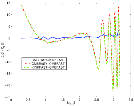
Figure 14: Relative difference of CMB spectrum for a rapidly varying dark energy model computed with CMBEASY, KINKFAST 1.0.0 and CMBFAST 4.5.1.

We find a perfect agreement within $1\%$. On the other hand we notice that the current version of CMBFAST 4.5.1, which implements the dark energy by reading a redshift sampled equation of state, leads to wrong spectra in the case of dark energy models with a rapid evolution in the equation of state (see figure 14). The cause of such a discrepancy is that the dark energy density is obtained through a splint integration procedure of the sampled equation of state. We find this method to be of poor accuracy. Without an analytic formula for $w(z)$, it is more reliable to derive a polynomial fitting function for the sampled equation of state and integrate the corresponding polynomial form with standard Numerical Recipes num integration subroutines such as rombint.

References

- (1) A. Riess et al., Astron. J. 116, 1009 (1998); S.J. Perlmutter at al., Astrophys. J. 517, 565 (1999).
- (2) G. Efstathiou et al., astro-ph/0109152.
- (3) D.N. Spergel et al., Astrophys. J. Suppl. 148, 175 (2003).
- (4) S.W. Allen, R.W. Schmidt, H. Ebeling, A.C. Fabian and L. van Speybroeck, astro-ph/0405340.
- (5) S. Weinberg, Rev. Mod. Phys. 61, 1 (1989).
- (6) C. Wetterich, Nucl. Phys. B 302, 668 (1988).
- (7) B. Ratra and P.J.E. Peebles, Phys. Rev. D37, 3406 (1988).
- (8) I. Zlatev, L. Wang and P.J. Steinhardt, Phys. Rev. Lett. 82, 896 (1999).
- (9) P.J. Steinhardt, L. Wang and I. Zlatevm, Phys. Rev. D59, 123504 (1999).
- (10) C. Armendáriz-Picón, V. Mukhanov, and P. J. Steinhardt, Phys. Rev. Lett. 85, 4438 (2000).
- (11) L. Amendola, Phys. Rev. D62, 043511 (2000).
- (12) L. Amendola and D. Tocchini-Valentini, Phys. Rev. D64, 043509 (2001).
- (13) M. Gasperini, F. Piazza and G. Veneziano, Phys. Rev. D65, 023508 (2002).
- (14) J. Khoury and A. Weltman, astro-ph/0309300.
- (15) A. Yu. Kamenshchik, U. Moschella and V. Pasquier, Phys. Lett. B511, 265 (2001).
- (16) K. Freese and L. Matthew, Phys. Lett. B540, 1 (2002), astro-ph/0201229.
- (17) B.A. Bassett, M. Kunz, D. Parkinson and C. Ungarelli, Phys. Rev. D68, 043504 (2003), astro-ph/0211303.
- (18) P.S. Corasaniti and E.J. Copeland, Phys. Rev. D65, 043004 (2002).
- (19) C. Baccigalupi, A. Balbi, S. Matarrese, F. Perrotta and N. Vittorio, Phys. Rev. D65, 063520 (2002).
- (20) R. Bean and A. Melchiorri, Phys. Rev. D65, 041302 (2002), astro-ph/0110472.
- (21) S. Hannestad and E. Mortsell, Phys. Rev. D66, 063508 (2002), astro-ph/0205096.
- (22) L. Amendola, C. Quercellini, D. Tocchini-Valentini and A. Pasqui, Astrophys. J. 583, L53 (2003).
- (23) B.A. Bassett, M. Kunz, J. Silk and C. Ungarelli, Mon. Not. Roy. Astron. Soc. 336, 1217 (2002).
- (24) C.L. Bennet et al., Astrophys. J. Suppl. 148, 1 (2003).
- (25) Riess et al. 2004 SN data.
- (26) P.S. Corasaniti and E.J. Copeland, Phys. Rev. D67, 063521 (2003), astro-ph/0205544.
- (27) B.A. Bassett, P.S. Corasaniti and M. Kunz, astro-ph/0407364.
- (28) P.S. Corasaniti, B.A. Bassett, C. Ungarelli and E.J. Copeland, Phys. Rev. Lett. 90, 091303 (2003), astro-ph/0210209.
- (29) U. Seljak and M. Zaldarriaga, Astrophys. J. 469, 437 (1996), astro-ph/9603033.
- (30) W. Freedman et al., Astrophys. J. 553, 47 (2001).
- (31) M. Colless et al., Mon. Not. Roy. Astron. Soc. 328, 1039 (2001).
- (32) M. Doran and M. Lilley, Mon. Not. Roy. Astron. Soc. 330, 965 (2002), astro-ph/0104486.
- (33) M. Doran, J.M. Schwindt and C. Wetterich, Phys. Rev. D64, 123520 (2001), astro-ph/0107525.
- (34) S. Burles, K.M. Nollett and M.S. Turner, Astrophys. J. 552, L1 (2001).
- (35) M. Kunz, P.S. Corasaniti, D. Parkinson and E.J. Copeland, astro-ph/0307346.
- (36) L. Verde et al., Astrophys. J. Suppl. 148, 195 (2003), astro-ph/0302218.
- (37) M. Tegmark, A.J.S. Hamilton and Y. Xu, Mon. Not. Roy. Astron. Soc. 335, 887 (2002), astro-ph/0111575.
- (38) W.R. Gilks, S. Richardson and D.J. Spiegelhalter, Markov chain Monte Carlo in practice, London: Chapman Hall.
- (39) J. Dunkley, M. Bucher, P.G. Ferreira, K. Moodley and C. Skordis, astro-ph/0405462.
- (40) Tegmark et al., Phys. Rev. D69, 103501 (2004), astro-ph/0310723.
- (41) U. Alam, V. Sahni, T.D. Saini and A.A. Starobinsky, astro-ph/0311364; U. Alam, V. Sahni and A.A. Starobinsky, J. Cosmol. Astropart. Phys. 06, 008 (2004), astro-ph/0403687.
- (42) S. Nesseris, L. Perivolaropoulos, astro-ph/0401556; B. Feng, X. Wang and X. Zhang, astro-ph/0404224.
- (43) D. Huterer and A. Cooray, astro-ph/0404062.
- (44) A. Slosar, U. Seljak and A. Makarov, astro-ph/0403073.
- (45) A.R. Liddle, astro-ph/0401198.
- (46) H. Akaike, IEEE Trans. Auto. Control, 19, 716 (1974).
- (47) G. Schwarz, Annals of Statistics, 5, 461 (1978).
- (48) W.J. Percival et al., Mont. Roy. Astron. Soc. 327, 1297 (2001), astro-ph/0105252.
- (49) S.W. Allen, R.W. Schimdt and A.C. Fabian, Mont. Not. Roy. Astron. Soc. 334, L11 (2002), astro-ph/0205007.
- (50) R.R. Caldwell and M. Doran, astro-ph/0305334.
- (51) Y. Wang and M. Tegmark, Phys. Rev. Lett. 92, 241302 (2004), astro-ph/0403292.
- (52) R.R. Caldwell et al., Astrophys. J. 591, L75 (2003).
- (53) T. Barreiro, E.J. Copeland and N.J. Nunes, Phys. Rev. D61, 127301 (2000), astro-ph/9910214.
- (54) A. Albrecht and C. Skordis, Phys. Rev. D64, 023514 (2001), astro-ph/9908085.
- (55) P. Brax and J. Martin, Phys. Lett. B468, 40 (1999), astro-ph/9905040.
- (56) A. de la Macorra and C. Stephan-Otto, Phys. Rev. D65, 083520 (2002), astro-ph/0110460.
- (57) J.P. Kneller and L.E. Strigari, Phys. Rev. D68, 083517 (2003), astro-ph/0302167.
- (58) L. Parker and A. Raval, Phys. Rev. D60, 123502 (1999).
- (59) A.C. Pope et al., astro-ph/0401249.
- (60) R.R. Caldwell, Phys. Lett. B545, 23 (2002), astro-ph/990816.
- (61) A. Melchiorri, L. Mersini, C.J. Odman and M. Trodden, astro-ph/0211522.
- (62) R.R. Caldwell, M. Kamionkowski and N.N. Weinberg, Phys. Rev. Lett. 91, 071301 (2003), astro-ph/0302506.
- (63) J. Weller, A.M. Lewis, Mont. Roy. Astron. Soc. 346, 987 (2003), astro-ph/0307104.
- (64) I. Maor, R. Brustein, J. McMahon and P.J. Steinhardt, Phys. Rev. D65, 123003 (2002), astro-ph/0112526.
- (65) J.-M. Virey, P. Taxil, A. Tilquin, A. Ealet, D. Fouchez and C. Tao, astro-ph/0403285.
- (66) S.M. Carroll, M. Hoffman and M. Trodden, Phys. Rev. D68, 023509 (2003), astro-ph/0301273; J.M. Cline, S. Jeon and G.D. Moore, hep-ph/0311312.
- (67) F. Giovi, C. Baccigalupi and F. Perrotta, Phys. Rev. D68, 123002 (2003), astro-ph/0308118.
- (68) M. Kamionkowski, A. Loeb, Phys.Rev. D56, 4511 (1997); J. Portsmouth, astro-ph/0402173; C. Skordis, J. Silk, astro-ph/0402474.
- (69) B.F. Gerke and G. Efstathiou, Mon. Not. Roy. Astron. Soc. 335, 33 (2002), astro-ph/0201336.
- (70) J. Weller and A. Albrecht, Phys. Rev. Lett. 86, 1939 (2001), astro-ph/0008314
- (71) E.V. Linder, Phys. Rev. Lett. 90, 091301 (2003), astro-ph/0208512.
- (72) H.K. Jassal, J.S. Bagla and T. Padmanabhan, astro-ph/0404378.
- (73) R. Bean, S.H. Hansen and A. Melchiorri, Phys. Rev. D64, 103508 (2001), astro-ph/0104162.
- (74) R. Dave, R.R. Caldwell and P.J. Steinhardt, Phys. Rev. D66, 023516 (2002), astro-ph/0206372.
- (75) M. Doran, astro-ph/0302138, http://www.cmbeasy.org/.
- (76) W.H. Press et al., Numerical Recipes in Fortran 77: The Art of Scientific Computing, Cambridge University Press.