A high-significance detection of non-Gaussianity in the WMAP 1-year data using directional spherical wavelets

Abstract

A directional spherical wavelet analysis is performed to examine the Gaussianity of the Wilkinson Microwave Anisotropy Probe (WMAP) 1-year data. Such an analysis is facilitated by the introduction of a fast directional continuous spherical wavelet transform. The directional nature of the analysis allows one to probe orientated structure in the data. Significant deviations from Gaussianity are detected in the skewness and kurtosis of spherical elliptical Mexican hat and real Morlet wavelet coefficients for both the WMAP and Tegmark et al. (2003) foreground-removed maps. The previous non-Gaussianity detection made by Vielva et al. (2003) using the spherical symmetric Mexican hat wavelet is confirmed, although their detection at the 99.9% significance level is only made at the 95.3% significance level using our most conservative statistical test. Furthermore, deviations from Gaussianity in the skewness of spherical real Morlet wavelet coefficients on a wavelet scale of $550\arcmin$ (corresponding to an effective global size on the sky of $\sim 26^{\circ}$ and an internal size of $\sim 3^{\circ}$) at an azimuthal orientation of $72^{\circ}$, are made at the 98.3% significance level, using the same conservative method. The wavelet analysis inherently allows one to localise on the sky those regions that introduce skewness and those that introduce kurtosis. Preliminary noise analysis indicates that these detected deviation regions are not atypical and have average noise dispersion. Further analysis is required to ascertain whether these detected regions correspond to secondary or instrumental effects, or whether in fact the non-Gaussianity detected is due to intrinsic primordial fluctuations in the cosmic microwave background.

1 Introduction

A range of primordial processes may imprint signatures on the temperature fluctuations of the cosmic microwave background (CMB). The currently favoured cosmological model is based on the assumption of initial fluctuations generated by inflation. In the simplest inflationary models, these result in Gaussian temperature anisotropies in the CMB. Non-standard inflationary models and various cosmic defect scenarios could, however, lead to non-Gaussian primordial CMB fluctuations. Non-Gaussianity may also be introduced by secondary effects, such as the reionisation of the Universe, the integrated Sachs-Wolfe effect, the Rees-Sciama effect, the Sunyaev-Zel’dovich effect and gravitational lensing – in addition to measurement systematics or foreground contamination. Consequently, probing the microwave sky for non-Gaussianity is of considerable interest, providing evidence for competing scenarios of the early Universe and also highlighting important secondary sources of non-Gaussianity and systematics.

Ideally, one would like to localise any detected non-Gaussian components on the sky, in particular to determine if they correspond to secondary effects or systematics. The ability to probe different scales is also important to ensure non-Gaussian sources present only on certain scales are not concealed by the predominant Gaussianity of other scales. Wavelet techniques are thus a perfect candidate for CMB non-Gaussianity analysis, since they provide both scale and spatial localisation. In addition, directional wavelets may provide further information on orientated structure in the CMB.

Wavelets have already been used to analyse the Gaussianity of the CMB. For example, Hobson et al. (1999) and Barreiro & Hobson (2001) investigated the use of planar wavelets in detecting and characterising non-Gaussianity on patches of the CMB sky. This approach was used by Mukherjee et al. (2000) to analyse planar faces of the 4-year Cosmic Background Explorer–Differential Microwave Radiometer (COBE-DMR) data in the QuadCube pixelisation, showing that the data is consistent with Gaussianity (correcting an earlier claim of non-Gaussianity by Pando et al. 1998). To consider a full sky CMB map properly, however, wavelet analysis must be extended to spherical geometry. A spherical Haar wavelet analysis of the COBE-DMR data was performed by Barreiro et al. (2000), but no evidence of non-Gaussianity was found. Employing the approach described by Antoine & Vandergheynst (1998) for performing continuous wavelet transforms on a sphere, Cayón et al. (2001) used the isotropic Mexican hat wavelet to analyse the COBE-DMR maps; again, no significant deviations from Gaussianity were detected. Martinez-González et al. (2002) subsequently compared the performance of spherical Haar and Mexican hat wavelets for non-Gaussianity detection and found the Mexican hat wavelet to be superior.

Since the release of the Wilkinson Microwave Anisotropy Probe (WMAP) 1-year data, a wide range of Gaussianity analyses have been performed, calculating measures such as the bispectrum and Minkowski functionals (Komatsu et al., 2003; Magueijo & Medeiros, 2004; Land & Magueijo, 2004), the genus (Colley & Gott, 2003; Eriksen et al., 2004), the 3-point correlation function (Gaztanaga & Wagg, 2003), multipole alignment statistics (, Copi et al.2004; de Oliveira-Costa et al., 2004; Slosar & Seljak, 2004), phase associations (Chiang et al., 2003; Coles et al., 2004), local curvature (Hansen et al., 2004; Cabella et al., 2004) and hot and cold spot statistics (Larson & Wandelt, 2004). Some statistics show consistency with Gaussianity, whereas others provide some evidence for a non-Gaussian signal and/or an asymmetry between the northern and southern Galactic hemispheres. One of the highest significance levels for non-Gaussianity yet reported was obtained by Vielva et al. (2003) using a spherical Mexican hat wavelet analysis. This result has been confirmed by Mukherjee & Wang (2004), who show it to be robust to different Galactic masks and assumptions regarding noise properties. In particular, it was found that the kurtosis of the wavelet coefficients in the southern hemisphere, at an approximate size on the sky of $10^{\circ}$, lies just outside the $3\sigma$ Gaussian confidence level.

Previous wavelet analyses of the CMB have been restricted to rotationally symmetric wavelets. A directional analysis on the full sky has previously been prohibited by the computational infeasibility of any implementation. In this paper, by applying a fast directional continuous spherical wavelet transform (CSWT), we extend non-Gaussianity analysis to examine directional structure in the CMB.

The remainder of this paper is structured as follows. The directional CSWT and the construction of new directional spherical wavelets is presented in Section 2. In Section 3 the procedure followed to analyse the WMAP 1-year data for non-Gaussianity is described. Results and further analysis are presented in Section 4. Concluding remarks are made in Section 5.

2 Directional continuous spherical wavelet analysis

To perform a wavelet analysis of full sky maps defined on the celestial sphere, Euclidean wavelet analysis must be extended to spherical geometry. We consider the directional CSWT constructed by Antoine & Vandergheynst (1998). This transform was constructed from group theoretic principles, however we present here an equivalent construction based on a few simple operations and norm-preserving properties.

2.1 Transform

A wavelet basis is constructed on the sphere by applying the spherical extension of Euclidean motions and dilations to mother wavelets defined on the sphere – analogous to the construction of a Euclidean wavelet basis.

The natural extension of Euclidean motions on the sphere are rotations. These are characterised by the elements of the rotation group $\mathrm{SO}(3)$, which we parameterise in terms of the three Euler angles $(\alpha,\beta,\gamma)$. The rotation of a square-integrable function $f$ on the 2-sphere $S^{2}$ (i.e. $f\in L^{2}(S^{2})$) is defined by

$$(\mathcal{R}_{\rho}f)(\omega)=f(\rho^{-1}\omega),\;\;\rho\in\mathrm{SO}(3)\>,$$ (1)

where $\omega$ denotes spherical coordinates (i.e. $\omega\in S^{2}$).

Dilations on the sphere are constructed by first lifting $S^{2}$ to the plane by a stereographic projection from the south pole (Figure 1), followed by the usual Euclidean dilation in the plane, before re-projecting back onto $S^{2}$. A spherical dilation is thus defined by

$$(\mathcal{D}_{a}f)(\omega)=f_{a}(\omega)=\sqrt{\lambda(a,\theta)}\>f(\omega_{1/a}),\;\;a\in\mathbb{R}^{+}_{\ast}\>,$$ (2)

where $\omega_{a}=(\theta_{a},\phi)$ and $\tan(\theta_{a}/2)=a\tan(\theta/2)$. The $\lambda(a,\theta)$ cocycle term is introduced to preserve the 2-norm and is defined by

$$\lambda(a,\theta)=\frac{4\>a^{2}}{[(a^{2}-1)\cos{\theta}+(a^{2}+1)]^{2}}\>.$$

\psfrag{x}{$x$}\psfrag{y}{$y$}\psfrag{z}{$z$}\psfrag{t}{$2\tan(\theta/2)$}\psfrag{a}{$\theta$}\includegraphics[width=159.33542pt]{figures/stereographic_projection_3d.eps}

Figure 1: Stereographic projection of the sphere onto the plane.

A wavelet basis on the sphere may now be constructed by rotations and dilations of an admissible mother spherical wavelet $\psi\in L^{2}(S^{2})$ (described further in Section 2.2). The corresponding wavelet family $\{\psi_{a,\rho}\equiv\mathcal{R}_{\rho}\mathcal{D}_{a}\psi,\;{\rho\in\mathrm{SO}(3),}\;{a\in\mathbb{R}_{\ast}^{+}}\}$ provides an over-complete set of functions in $L^{2}(S^{2})$. The CSWT of $s\in L^{2}(S^{2})$ is given by the projection onto each wavelet basis function in the usual manner,

$$W(a,\alpha,\beta,\gamma)=\int_{S^{2}}(\mathcal{R}_{\alpha,\beta,\gamma}\psi_{a})^{\ast}(\omega)\;s(\omega)\>\mathrm{\,d}\mu(\omega)\>,$$ (3)

where the $\ast$ denotes complex conjugation and $\mathrm{\,d}\mu(\omega)=\sin(\theta)\mathrm{\,d}\theta\mathrm{\,d}\phi$ is the usual rotationally invariant measure on the sphere.

The transform is general in the sense that all orientations in the rotation group $\mathrm{SO}(3)$ are considered, thus directional structure is naturally incorporated. It is important to note, however, that only local directions make any sense on $S^{2}$. There is no global way of defining directions on the sphere – there will always be some singular point where the definition fails.

A full directional wavelet analysis on the sphere has previously been prohibited by the computational infeasibility of any implementation. We rectify this problem by presenting a fast algorithm in Appendix A to perform the directional CSWT.

2.2 Mother spherical wavelets

The wavelet basis previously described is constructed from rotations and dilations of an admissible mother spherical wavelet. Mother spherical wavelets are simply constructed by projecting admissible Euclidean planar wavelets onto the sphere by an inverse stereographic projection,

$$\psi_{S^{2}}(\theta,\phi)=(\Pi^{-1}\psi_{\mathbb{R}^{2}})(\theta,\phi)\equiv\frac{2}{1+\cos(\theta)}\>\psi_{\mathbb{R}^{2}}(r,\phi)\>,$$ (4)

where $r=2\tan(\theta/2)$. The modulating term is again introduced to preserve the 2-norm.

Directional spherical wavelets may be naturally constructed in this setting – they are simply the projection of directional Euclidean planar wavelets onto the sphere. Two directional planar Euclidean mother wavelets are defined in the following subsections: the elliptical Mexican hat and real Morlet wavelets. The corresponding spherical wavelets are illustrated in Figure 2. The Mexican hat wavelet and the real Morlet wavelet, chosen for its sensitivity to scanning artifacts, are subsequently applied to the detection of non-Gaussianity in the WMAP 1-year data.

   

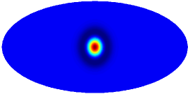
(a) Mexican hat $\epsilon=0.00$

(b) Mexican hat $\epsilon=0.95$

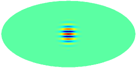
(c) Real Morlet $\mn@boldsymbol{k}=\left(10,0\right)^{T}$

Figure 2: Spherical wavelets (dilation $a=750\arcmin$; size on sky $\xi_{1}=2100\arcmin$, $\xi_{2}=236\arcmin$).

2.2.1 Elliptical Mexican hat wavelet

We propose a directional extension of the usual Mexican hat wavelet. The elliptical Mexican hat wavelet is defined as the negative of the Laplacian of an elliptical 2-dimensional Gaussian,

$$\psi_{\mathbb{R}^{2}}^{\rm Mex}(x,y;\sigma_{x},\sigma_{y})=\frac{1}{2\pi\sigma_{x}^{3}\sigma_{y}^{3}}\left(\sigma_{x}^{2}+\sigma_{y}^{2}-\frac{x^{2}}{(\sigma_{x}/\sigma_{y})^{2}}-\,\frac{y^{2}}{(\sigma_{y}/\sigma_{x})^{2}}\right)$$ (5)

$$\times\>\exp\left[-\frac{1}{2}\left(\frac{x^{2}}{\sigma_{x}^{2}}+\frac{y^{2}}{\sigma_{y}^{2}}\right)\right]\>,$$

which reduces to the usual symmetric Mexican hat wavelet for the special case where $\sigma_{x}=\sigma_{y}$. The elliptical Mexican hat wavelet is invariant under integer azimuthal rotations of $\pi$, thus the rotation angle $\gamma$ is always quoted in the range $[0,\pi)$.

We define the eccentricity of an elliptical Mexican hat wavelet as the eccentricity of the ellipse defined by the first zero-crossing, given by

$$\epsilon=\sqrt{1-\left(\frac{\sigma_{y}}{\sigma_{x}}\right)^{4}}\>.$$ (6)

Elliptical Mexican hat wavelets are subsequently parameterised by their eccentricity; the standard deviation in each direction is set by $\sigma_{y}=1$ and $\sigma_{x}=\sigma_{y}\sqrt[4]{1-\epsilon^{2}}$. Elliptical Mexican hat wavelets are illustrated in Figure 2 (a) and (b) for eccentricities $\epsilon=0.00$ and $\epsilon=0.95$ respectively.

We define the effective size on the sky of a spherical elliptical Mexican hat wavelet for a particular dilation as the angular separation between the first zero-crossings on the major axis of the ellipse, given by

$$\xi^{\rm Mex}_{1}(a)=4\tan^{-1}\left(\frac{a}{\sqrt{2}}\right)\approx 2\sqrt{2}\>a\>.$$ (7)

2.2.2 Real Morlet wavelet

The real Morlet wavelet is defined by

$$\psi_{\mathbb{R}^{2}}^{\rm Mor}(\mn@boldsymbol{x};\mn@boldsymbol{k})=\rm{Re}\left[\exp\left(\frac{\mathit{i}\>\mn@boldsymbol{k}\cdot\mn@boldsymbol{x}}{\sqrt{2}}\right)\exp\left(\frac{-\|\mn@boldsymbol{x}\|^{2}}{2}\right)\right]\>,$$ (8)

where $\mn@boldsymbol{k}$ is the wave vector of the wavelet (henceforth we consider only wave vectors of the form $\mn@boldsymbol{k}=\left(k_{0},0\right)^{T}$). We have scaled the usual definition of the real Morlet wavelet to achieve size consistency with the elliptical Mexican hat wavelet. The real Morlet spherical wavelet is also invariant under integer azimuthal rotations of $\pi$, thus the rotation angle $\gamma$ is always quoted in the domain $[0,\pi)$.

The real Morlet wavelet has two orthogonal scales: one defining the overall size of the wavelet and the other defining the size of its internal structure. The overall effective size on the sky of the spherical real Morlet wavelet is defined as the angular separation between opposite $e^{-1}$ roll-off points of the exponential decay factor, and is given by

$$\xi^{\rm Mor}_{1}(a)=4\tan^{-1}\left(\frac{a}{\sqrt{2}}\right)\approx 2\sqrt{2}\>a\>.$$ (9)

Notice that for a given dilation $a$, the spherical elliptical Mexican hat and real Morlet wavelets have an equivalent overall effective size on the sky. The effective size on the sky of the internal structure of the real Morlet wavelet is defined as the angular separation between the first zero-crossings in the direction of the wave vector $\mn@boldsymbol{k}$, and is given by

$$\xi^{\rm Mor}_{2}(a)=4\tan^{-1}\left(\frac{a\pi}{4k_{0}}\right)\approx\frac{a\pi}{k_{0}}\>.$$ (10)

3 Non-Gaussianity analysis

Spherical wavelet analysis is applied to probe the WMAP 1-year data for possible deviations from Gaussianity. We follow a similar strategy to Vielva et al. (2003), however we extend the analysis to directional spherical wavelets to probe orientated structure in the CMB.

3.1 Data preprocessing

We consider the same data set analysed by both Komatsu et al. (2003) and Vielva et al. (2003) in their non-Gaussianity studies. The observed WMAP maps for which the CMB is the dominant signal (two Q-band maps at 40.7GHz, two V-band maps at 60.8GHz and four W-band maps at 93.5GHz) are combined to give a single signal-to-noise ratio enhanced map. These maps, together with receiver noise and beam properties, are available from the Legacy Archive for Microwave Background Data Analysis (LAMBDA) website. The maps are provided in the HEALPix (Górski et al., 1999) format at a resolution of ${N_{side}}=512$ (the number of pixels in a HEALPix map is given by $12\,{N_{side}}^{2}$). The data processing pipeline specified by Komatsu et al. (2003) is applied to produce a single co-added map for analysis. The co-added temperature at a given position on the sky $\omega$ is given by

$$T(\omega)=\frac{\sum_{r=3}^{10}w_{r}(\omega)\>T_{r}(\omega)}{\sum_{r=3}^{10}w_{r}(\omega)}\>,$$ (11)

where $T(\omega)$ is a CMB temperature map and the $r$ index corresponds to the Q-, V- and W-band receivers respectively (indices $r=1,2$ correspond to the K and Ka receiver bands that are excluded from the analysis). The noise weights $w_{r}(\omega)$ are defined by

$$w_{r}(\omega)=\frac{N_{r}(\omega)}{{\sigma_{0_{r}}}^{2}}\>,$$ (12)

where $N_{r}(\omega)$ specifies the number of observations at each point on the sky for each receiver band and $\sigma_{0_{r}}$ is the receiver noise dispersion.

Foreground cleaned sky maps, where the Galactic foreground signal (consisting of synchrotron, free-free, and dust emission) has been removed, are directly available from the LAMBDA website. The Galactic foreground signal is removed by using the 3-band, 5-parameter template fitting method described by Bennett et al. (2003). We use these foreground cleaned maps in our analysis.

An independent foreground analysis of the WMAP data is performed by Tegmark et al. (2003). The Tegmark et al. map is also constructed from a linear summation of observed WMAP maps, however the weights used vary over both position on the sky and scale. We also perform our analysis on the Tegmark et al. map to ensure any detected deviations from Gaussianity are not due to differences in the various foreground removal techniques.

Following the analysis of Vielva et al. (2003) we down-sample map resolutions to ${N_{side}}=256$, since the very small scales are dominated by noise (and also to reduce computational requirements). The conservative Kp0 exclusion mask provided by the WMAP team (appropriately downsampled to conserve point source exclusion regions in the coarser resolution) is applied to remove emissions due to the Galactic plane and known point sources. The final preprocessed co-added map (hereafter referred to as the WMAP team map, or simply WMAP map) and the map produced by Tegmark et al. (2003) (hereafter referred to as the Tegmark map) are illustrated in Figure 3.

 

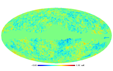
(a) Co-added WMAP team map

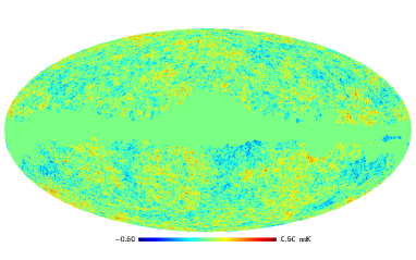
(b) Tegmark map

Figure 3: Preprocessed WMAP maps considered in the non-Gaussianity analysis.

3.2 Monte Carlo simulations

Monte Carlo simulations are performed to construct confidence bounds on the test statistics used to probe for non-Gaussianity in the WMAP 1-year data. 1000 Gaussian CMB realisations are produced from the theoretical power spectrum fitted by the WMAP team.

To simulate the WMAP observing strategy each Gaussian CMB realisation is convolved with the beam transfer function of each of the Q-, V- and W-band receivers. White noise of dispersion $\sigma_{r}(\omega)=\sigma_{0_{r}}/\sqrt{N_{r}(\omega)}$ is added to each band. The resultant simulated Q-, V- and W-band maps are combined in the same manner used to construct the co-added map, before down-sampling and applying the Kp0 mask, to give a final simulated Gaussian co-added map for analysis.

The same Gaussian simulations are also used for comparison with the Tegmark map. Since the weights used to construct the Tegmark map differ from those used to construct the WMAP team map, one should strictly produce a second set of Gaussian simulations following the Tegmark map construction method. The weights for the Tegmark map vary as a function of angular scale, and unfortunately are not quoted explicitly. Nevertheless, for both the WMAP and Tegmark maps, the weights sum to unity and the difference in the linear combination of maps used by Tegmark et al. (2003) should not lead to significant changes in the Gaussian confidence limits as compared with those obtained using the Gaussian simulations produced to model the WMAP map.

3.3 Wavelet analysis

The CSWT is a linear operation; hence the wavelet coefficients of a Gaussian map will also follow a Gaussian distribution. One may therefore probe a full sky CMB map for non-Gaussianity simply by looking for deviations from Gaussianity in the distribution of the spherical wavelet coefficients.

The analysis consists of first taking the CSWT at a range of scales and, for directional wavelets on the sphere, a range of $\gamma$ directions. The scales we consider (and the corresponding effective size on the sky for both the Mexican hat and real Morlet wavelets) are shown in Table 1. For directional wavelets we consider five evenly spaced $\gamma$ orientations in the domain $[0,\pi)$.

Table 1: Wavelet scales considered in the non-Gaussianity analysis. The overall size on the sky $\xi_{1}$ for a given scale are the same for both the Mexican hat and real Morlet wavelets. The size on the sky of the internal structure of the real Morlet wavelet $\xi_{2}$ is also quoted.

Scale	1	2	3	4	5	6	7	8	9	10	11	12
Dilation $a$	50′	100′	150′	200′	250′	300′	350′	400′	450′	500′	550′	600′
Size on sky $\xi_{1}$	141′	282′	424′	565′	706′	847′	988′	1130′	1270′	1410′	1550′	1690′
Size on sky $\xi_{2}$	15.7′	31.4′	47.1′	62.8′	78.5′	94.2′	110′	126′	141′	157′	173′	188′

Those wavelet coefficients distorted by the application of the Kp0 mask are removed, as subsequently described, before test statistics are calculated from the wavelet coefficients. An identical analysis is performed on each Monte Carlo CMB simulation in order to construct significance measures for the test statistics.

3.3.1 Coefficient exclusion masks

The application of the Kp0 exclusion mask distorts coefficients corresponding to wavelets that overlap with the mask exclusion region. These contaminated wavelet coefficients must be removed from any subsequent non-Gaussianity analysis. An extended coefficient exclusion mask is required to remove all contaminated wavelet coefficients.

On small scales masked point sources introduce significant distortion in wavelet coefficient maps and should not be neglected. On larger scales the masked Galactic plane introduces the most significant distortion, as point source distortions are averaged over a large wavelet support. Our construction of an extended coefficient mask inherently accounts for the dominant type of distortion on a particular scale. Firstly, the CSWT of the original Kp0 mask is taken. Admissible spherical wavelets have zero mean (Antoine et al., 2002), hence the only non-zero wavelet coefficients are those that are distorted by the mask boundary. These distorted coefficients may be easily detected and the coefficient exclusion mask extended accordingly. Coefficient exclusion masks are illustrated in Figure 4 for the Mexican hat $\epsilon=0.00$ wavelet for a range of scales and in Figure 5 for the real Morlet wavelet for a given scale (the scale that a significant non-Gaussianity detection is subsequently made) and a range of orientations. As scale increases the dominant form of distortion may be seen in Figure 4 to shift from point source to Galactic plane.

Vielva et al. (2003) construct an extended coefficient mask simply by extending the Galactic plane region of the Kp0 mask by $2.5a$ (the point source components of the original mask are not extended). Several other definitions for coefficient exclusion masks are analysed in detail by Mukherjee & Wang (2004), none of which alter the results of subsequent non-Gaussianity analysis. Although it is important to account correctly for the distortions introduced by the Kp0 mask, the results of Gaussianity analysis appear to be relatively insensitive to the particular mask chosen.

               

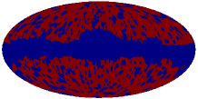
(a) $a_{1}=50\arcmin$

(b) $a_{2}=100\arcmin$

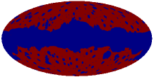
(c) $a_{3}=150\arcmin$

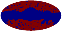
(d) $a_{4}=200\arcmin$

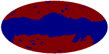
(e) $a_{5}=250\arcmin$

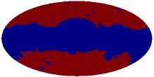
(f) $a_{6}=300\arcmin$

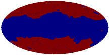
(g) $a_{7}=350\arcmin$

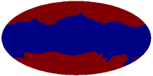
(h) $a_{8}=400\arcmin$

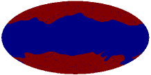
(i) $a_{9}=450\arcmin$

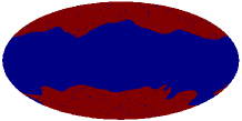
(j) $a_{10}=500\arcmin$

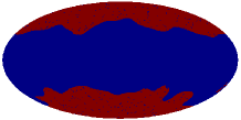
(k) $a_{11}=550\arcmin$

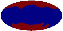
(l) $a_{12}=600\arcmin$

Figure 4: Symmetric Mexican hat $\epsilon=0.00$ wavelet coefficient exclusion masks for each scale.

     

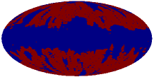
(a) $\gamma=0^{\circ}$

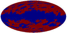
(b) $\gamma=72^{\circ}$

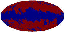
(c) $\gamma=144^{\circ}$

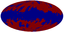
(d) $\gamma=216^{\circ}$

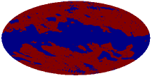
(e) $\gamma=288^{\circ}$

Figure 5: Real Morlet wavelet coefficient exclusion masks at scale $a_{11}=550\arcmin$ for each orientation.

3.3.2 Test statistics

The third (skewness) and fourth (kurtosis) moments about the mean are considered to test spherical wavelet coefficients for deviations from Gaussianity. These estimators describe the degree of symmetry and the degree of peakedness in the underlying distribution respectively. Skewness is defined by

$$\zeta(a,\gamma)=\frac{1}{N_{\rm eff}}\sum_{i=1}^{N_{\rm eff}}\frac{\left[\>W_{i}(a,\gamma)-\mu(a,\gamma)\>\right]^{3}}{\sigma^{3}(a,\gamma)}$$ (13)

and excess kurtosis by

$$\kappa(a,\gamma)=\frac{1}{N_{\rm eff}}\sum_{i=1}^{N_{\rm eff}}\frac{\left[\>W_{i}(a,\gamma)-\mu(a,\gamma)\>\right]^{4}}{\sigma^{4}(a,\gamma)}\>-\>3\>,$$ (14)

where $\mu$ is the mean and $\sigma$ the dispersion of the wavelet coefficients. The $i$ index ranges over all wavelet coefficients not excluded by the coefficient exclusion mask and indexes both $\alpha$ and $\beta$ components. The number of spherical wavelet coefficients retained in the analysis after the application of the coefficient exclusion mask is given by $N_{\rm eff}$.

Skewness and excess kurtosis for a Gaussian distribution are both zero. We look for deviations from zero in these test statistics to indicate the existence of non-Gaussianity in the distribution of spherical wavelet coefficients, and hence also in the corresponding CMB map.

4 Results

To probe for non-Gaussianity in the WMAP 1-year data, the analysis procedure described in Section 3 is performed on both the WMAP team and Tegmark maps. The three spherical wavelets illustrated in Figure 2 are considered, namely the symmetric Mexican hat $\epsilon=0.00$ wavelet, the elliptical Mexican hat $\epsilon=0.95$ wavelet and the real Morlet $\mn@boldsymbol{k}=\left(10,0\right)^{T}$ wavelet. The Mexican hat $\epsilon=0.00$ case has previously been analysed by Vielva et al. (2003) (although some scales considered differ), thereby providing a consistency check for the analysis.

4.1 Wavelet coefficient statistics

For a given wavelet, the skewness and kurtosis of wavelet coefficients is calculated for each scale and orientation. These statistics are displayed in Figure 6, with confidence intervals constructed from the Monte Carlo simulations also shown. For directional wavelets, only the orientations corresponding to the maximum deviations from Gaussianity are shown.

Our coefficient exclusion mask differs slightly from that applied by Vielva et al. (2003), thus for comparison purposes we also perform the Mexican hat $\epsilon=0.00$ analysis without applying any extended coefficient mask, as Vielva et al. (2003) also do initially. These results, although not shown, correspond identically. By applying different coefficient masks the shape of the plots differ slightly, nevertheless the findings drawn remain the same. Deviations from Gaussianity are detected in the kurtosis outside of the 99% confidence region constructed from Monte-Carlo simulations, on scales $a_{5}=250\arcmin$ and $a_{6}=300\arcmin$. Furthermore, a deviation outside the 99% confidence region is detected in the skewness at scale $a_{2}=100\arcmin$. Vielva et al. (2003) measure a similar skewness value at this scale, although this lies directly on the boundary of their 99% confidence region.

Deviations from Gaussianity are also detected in both skewness and kurtosis using the elliptical Mexican hat $\epsilon=0.95$ wavelet. In each case the observed deviations occur on a slightly larger scale than those found using the symmetric Mexican hat $\epsilon=0.00$ wavelet. This behaviour also appears typical for simulated Gaussian map realisations. Adjacent orientations exhibit similar results, although not at such large confidence levels (but still outside of the 99% confidence level).

An extremely significant deviation from Gaussianity is observed in the skewness of the real Morlet wavelet coefficients at scale $a_{11}=550\arcmin$ and orientation $\gamma=72^{\circ}$. The kurtosis measurement on the same scale and orientation also lies outside of the 99% confidence region.

       

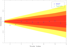
(a) Skewness – Mexican hat $\epsilon=0.00$

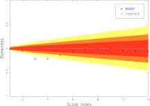
(b) Skewness – Mexican hat $\epsilon=0.95$; $\gamma=72^{\circ}$

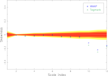
(c) Skewness – real Morlet $\mn@boldsymbol{k}=\left(10,0\right)^{T}$; $\gamma=72^{\circ}$

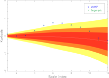
(d) Kurtosis – Mexican hat $\epsilon=0.00$

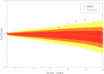
(e) Kurtosis – Mexican hat $\epsilon=0.95$; $\gamma=108^{\circ}$

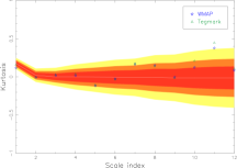
(f) Kurtosis – real Morlet $\mn@boldsymbol{k}=\left(10,0\right)^{T}$; $\gamma=72^{\circ}$

Figure 6: Spherical wavelet coefficient statistics for each wavelet. Confidence regions obtained from 1000 Monte Carlo simulations are shown for 68% (red), 95% (orange) and 99% (yellow) levels, as is the mean (solid white line). Only the orientations corresponding to the most significant deviations from Gaussianity are shown for the Mexican hat $\epsilon=0.95$ and real Morlet wavelet cases.

4.2 Statistical significance of detections

We now consider in more detail, the most significant deviation from Gaussianity obtained in each of the panels in Figure 6. In particular, we examine the distribution of each statistic, obtained from the Gaussian Monte Carlo simulations, and also perform a $\chi^{2}$ test for each statistic. Significance measures of the non-Gaussianity detections may then be constructed from each test.

Figure 7 shows histograms constructed from the Monte Carlo simulations for those test statistics corresponding to the most significant deviations from Gaussianity. The measured statistic for both the WMAP team and Tegmark maps is also shown on each plot, with the number of standard deviations these observations deviate from the mean. In particular, we note the large deviations shown in panel (c), corresponding to $5.61$ and $6.42$ standard deviations for the real Morlet wavelet analysis of the WMAP and Tegmark maps respectively.

       

(a) Skewness – Mexican hat $\epsilon=0.00$; $a_{2}=100\arcmin$

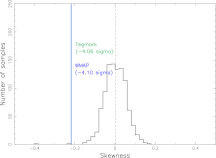
(b) Skewness – Mexican hat $\epsilon=0.95$; $a_{3}=150\arcmin$; $\gamma=72^{\circ}$

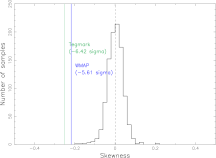
(c) Skewness – real Morlet $\mn@boldsymbol{k}=\left(10,0\right)^{T}$; $a_{11}=550\arcmin$; $\gamma=72^{\circ}$

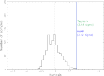
(d) Kurtosis – Mexican hat $\epsilon=0.00$, $a_{6}=300\arcmin$

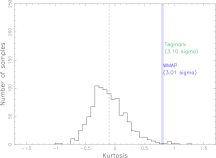
(e) Kurtosis – Mexican hat $\epsilon=0.95$; $a_{10}=500\arcmin$; $\gamma=108^{\circ}$

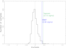
(f) Kurtosis – real Morlet $\mn@boldsymbol{k}=\left(10,0\right)^{T}$; $a_{11}=550\arcmin$; $\gamma=72^{\circ}$

Figure 7: Histograms of spherical wavelet coefficient statistic obtained from 1000 Monte Carlo simulations. The mean is shown by the dashed vertical line. The observed statistics for the WMAP and Tegmark maps are shown by the blue and green lines respectively. The number of standard deviations these observations deviate from the mean is also displayed on each plot. Only those scales and orientations corresponding to the most significant deviations from Gaussianity are shown for each wavelet.

Having determined separately the confidence level of the largest non-Gaussianity detection in each panel of Figure 6, we now consider the statistical significance of our results for each wavelet as a whole. Treating each wavelet separately, we search through the Gaussian simulations to determine the number of maps that have an equivalent or greater deviation in any of the test statistics calculated from that map using the given wavelet. That is, if any skewness or kurtosis statistic calculated from the Gaussian map – on any scale or orientation – deviates more than the maximum deviation observed in the WMAP data for that wavelet, then the map is flagged as exhibiting a more significant deviation. This is an extremely conservative means of constructing significance levels for the observed test statistics. Significance levels corresponding to the detections considered in Figure 7 are calculated and displayed in Table 2. Notice that although several individual test statistics fall outside of the 99% confidence region, the true significance level of the detection when all statistics are taken into account is considerably lower. Using our conservative test, the significance of the non-Gaussianity detection made by Vielva et al. (2003), previously quoted at greater than 99.9% significance, drops to a significance level of 95.3%. Of particular interest is the non-Gaussian detection in the skewness of real Morlet wavelet coefficients on scale $a_{11}=550\arcmin$ and orientation $\gamma=72^{\circ}$. This statistic deviates from the mean by $5.61$ standard deviations for the WMAP map and by $6.42$ standard deviations for the Tegmark map. The detection is made at an overall significance level of 98.3%.

Table 2: Deviation and significance levels of spherical wavelet coefficient statistics calculated from the WMAP map (similar results are obtained using the Tegmark map). Standard deviations and significant levels are calculated from 1000 Monte Carlo Gaussian simulations. The table variables are defined as follows: the number of standard deviations the observation deviates from the mean is given by $N_{\sigma}$; the number of simulated Gaussian maps that exhibit an equivalent or greater deviation in any test statistics calculated using the given wavelet is given by $N_{\rm dev}$; the corresponding significance level of the non-Gaussianity detection is given by $\delta$. Only those scales and orientations corresponding to the most significant deviations from Gaussianity are shown for each wavelet.

	Skewness	Kurtosis
	($a_{2}=100\arcmin$)	($a_{6}=300\arcmin$)
$N_{\sigma}$	$-3.38$	$3.12$
$N_{\rm dev}$	28 maps	47 maps
$\delta$	97.2%	95.3%

(a) Mexican hat $\epsilon=0.00$

	Skewness	Kurtosis
	($a_{3}=150\arcmin$; $\gamma=72^{\circ}$)	($a_{10}=500\arcmin$; $\gamma=108^{\circ}$)
$N_{\sigma}$	$-4.10$	$3.01$
$N_{\rm dev}$	39 maps	199 maps
$\delta$	96.1%	80.1%

(b) Mexican hat $\epsilon=0.95$

	Skewness	Kurtosis
	($a_{11}=550\arcmin$; $\gamma=72^{\circ}$)	($a_{11}=550\arcmin$; $\gamma=72^{\circ}$)
$N_{\sigma}$	$-5.61$	$2.66$
$N_{\rm dev}$	17 maps	642 maps
$\delta$	98.3%	35.8%

(c) Real Morlet $\mn@boldsymbol{k}=\left(10,0\right)^{T}$

The preceding analysis is based on the marginal distributions of individual statistics and makes a posterior selection of the critical confidence limit from the most discrepant values obtained from the data. A $\chi^{2}$ test provides an alternative analysis and method of constructing significance measures. This test instead considers the set of test statistics for each wavelet as a whole and hence is based on their joint distribution. The posterior statistic selection problem is thus eliminated, however including a large number of less useful test statistics has a pronounced effect on down-weighting the overall significance of the test. The $\chi^{2}$ statistic is given by

$$\chi^{2}=\sum_{i=1}^{N_{\rm stat}}\>\sum_{j=1}^{N_{\rm stat}}\>(\tau_{i}-\overline{\tau}_{i})\>(C^{-1})_{ij}\>(\tau_{j}-\overline{\tau}_{j})\>,$$ (15)

where $\tau_{i}$ gives each test statistic. For Gaussian distributed test statistics this should satisfy a $\chi^{2}$ distribution. Although our test statistics are not Gaussian distributed, one may still use the $\chi^{2}$ test if one is willing to estimate significance levels using Monte Carlo simulations. The test statistics include both skewness and kurtosis statistics for each scale and orientation, hence there are $24$ statistics for the symmetric Mexican hat analysis and $120$ for each of the directional wavelet analyses. The mean value for each test statistic $\overline{\tau}$ and the covariance matrix $C$ is calculated from the Gaussian simulations. $\chi^{2}$ values are calculated for the WMAP map, and also for all simulated Gaussian realisations. The previously described approach for constructing significance levels is applied to the $\chi^{2}$ statistics. Figure 8 summarises the results obtained. All spherical wavelet analyses flag deviations from Gaussianity of very high significance when all test statistics are incorporated in this manner. In particular, the detection made using the symmetric Mexican hat wavelet occurs at the 99.9% significance level and that made with the real Morlet wavelet occurs at the 99.3% significance level. In this case the superiority of the symmetric Mexican hat wavelet over the real Morlet wavelet arises since the real Morlet wavelet analysis contains a number of additional less useful statistics (due to the additional orientations), that dilute the overall results.

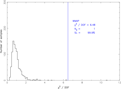
(d) Mexican hat $\epsilon=0.00$

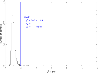
(e) Mexican hat $\epsilon=0.95$

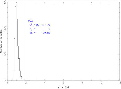
(f) Real Morlet $\mn@boldsymbol{k}=\left(10,0\right)^{T}$

Figure 8: Histograms of normalised $\chi^{2}$ test statistics obtained from 1000 Monte Carlo simulations. The normalised $\chi^{2}$ value obtained from the WMAP map is indicated by the blue vertical line (similar results are obtained using the Tegmark map). The number of simulated maps that exhibit a greater or equivalent $\chi^{2}$ value than the WMAP map is quoted ($N_{e}$), accompanied by the corresponding significance level (SL).

Since the first analysis is based on marginal distributions, as opposed to the joint distribution of statistics probed by the $\chi^{2}$ test, the former is more conservative. Thus we quote the overall significance of all detections of non-Gaussianity at the level calculated by the first method (which, in all cases, is the lower of the values calculated by the two methods).

4.3 Localised deviations from Gaussianity

Wavelet analysis inherently affords the spatial localisation of interesting signal characteristics. The most pronounced deviations from Gaussianity in the WMAP 1-year data may therefore be localised on the sky. In addition, directional wavelets also allow signal components to be localised in orientation.

The wavelet coefficients corresponding to the most significant non-Gaussian detections for each wavelet are displayed in Figure 9, accompanied by corresponding thresholded maps to localise the most pronounced deviations from Gaussianity. The regions displayed in Figure 9 (b) that are detected from the kurtosis Mexican hat $\epsilon=0.00$ analysis are in close accordance with those regions found by Vielva et al. (2003). Additional similarities appear to exist between the regions detected from different thresholded wavelet coefficient maps, as apparent in Figure 9. To quantify these similarities, the cross-correlation of all combinations of thresholded coefficient maps is computed (the cross-correlation is normalised to lie in the range $[-1,1]$, where unity indicates a fully correlated map). Table 3 shows the normalised cross-correlation values obtained. Deviation regions shown in Figure 9 (b) and Figure 9 (d), detected by the Mexican hat $\epsilon=0.00$ and $\epsilon=0.95$ wavelets respectively, are highly correlated. Interestingly, these coefficient maps are both flagged by excess kurtosis measures. Furthermore, the regions shown in Figure 9 (a) and Figure 9 (c), detected by the Mexican hat $\epsilon=0.00$ and $\epsilon=0.95$ wavelets respectively, are moderately correlated. These coefficient maps are both flagged by excess skewness measures. No other combinations of thresholded coefficient maps exhibit any significant similarities. In particular, the deviation regions detected by the skewness real Morlet analysis (Figure 9 (e)) do not correlate with any of the regions found using the Mexican hat wavelets. This is expected since a different wavelet that probes different structure is applied. The cross-correlation relationships exhibited here between detected deviation regions for the WMAP map, also appear typical of simulated Gaussian maps.

To investigate the impact of these localised regions on the initial non-Gaussianity detection, the corresponding coefficients are removed from the calculation of skewness and kurtosis test statistics. The non-Gaussian detections are substantially reduced for all of the six most significant test statistics considered in Figure 7. For the statistics considered in Figure 7 (c), (d) and (e) the detection of non-Gaussianity is completely eliminated. For the remaining cases considered in Figure 7 (a), (b) and (f) non-Gaussian detections are reduced in significance and lie between the 95% and 99% confidence levels.

Thus, the localised deviation regions identified do indeed appear to be the source of detected non-Gaussianity. Moreover, those detected regions shown in Figure 9 (a), (c) and (e) appear to introduce skewness into the WMAP map, whereas those detected regions shown in Figure 9 (b) and (d) appear to introduce kurtosis.

(Cruz et al.2004), in a continuation of the work of Vielva et al. (2003), consider localised regions in more detail and find the large cold spot at $(b=-57^{\circ},\;l=209^{\circ})$ to be the main source of non-Gaussianity detected by the symmetric Mexican hat wavelet analysis. A similar analysis may be performed using the wavelets we consider and the associated localised regions, although we leave this for a further work.

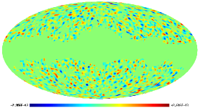
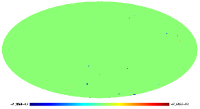
(a) Mexican hat $\epsilon=0.00$; $a_{2}=100\arcmin$

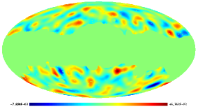
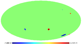
(b) Mexican hat $\epsilon=0.00$; $a_{6}=300\arcmin$

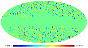
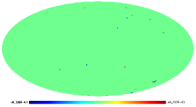
(c) Mexican hat $\epsilon=0.95$; $a_{3}=150\arcmin$; $\gamma=72^{\circ}$

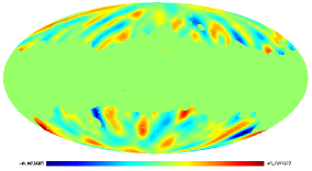
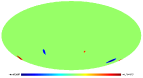
(d) Mexican hat $\epsilon=0.95$; $a_{10}=500\arcmin$; $\gamma=108^{\circ}$

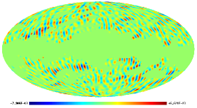
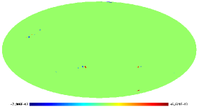
(e) Real Morlet $\mn@boldsymbol{k}=\left(10,0\right)^{T}$; $a_{11}=550\arcmin$; $\gamma=72^{\circ}$

Figure 9: Spherical wavelet coefficient maps (left) and thresholded maps (right). To localise most likely deviations from Gaussianity on the sky, the coefficient maps exhibiting strong non-Gaussianity are thresholded so that only those coefficients above $3\sigma$ (in absolute value) are shown. Due to the apparent similarity of the WMAP team and Tegmark maps, only coefficients for the analysis of the WMAP map are shown above.

Table 3: Normalised cross-correlation of thresholded spherical wavelet coefficient maps indicating the similarity between the localised most likely deviations from Gaussianity flagged by the most significant skewness and kurtosis observations for each wavelet. Notice that the regions detected from the skewness flagged maps of the symmetric and elliptical Mexican hat wavelets are moderately correlated, while the regions detected from the kurtosis flagged maps of the symmetric and elliptical Mexican hat wavelets are strongly correlated. The regions flagged by the real Morlet wavelet analysis are not correlated with any of the other regions detected by a Mexican hat wavelet analysis, as expected since a different wavelet that probes different structure is applied. (Note that the lettered key corresponds to the thresholded coefficient maps contained in the panels of Figure 9.)

Thresholded coefficient map		(a)	(b)	(c)	(d)	(e)
(a)	Mexican hat $\epsilon=0.00$	1.00	0.00	0.46	0.00	0.00
	$a_{2}=100\arcmin$
(b)	Mexican hat $\epsilon=0.00$	-	1.00	0.04	0.70	0.00
	$a_{6}=300\arcmin$
(c)	Mexican hat $\epsilon=0.95$	-	-	1.00	0.05	0.01
	$a_{3}=150\arcmin$; $\gamma=72^{\circ}$
(d)	Mexican hat $\epsilon=0.95$	-	-	-	1.00	0.00
	$a_{10}=500\arcmin$; $\gamma=108^{\circ}$
(e)	Real Morlet $\mn@boldsymbol{k}=\left(10,0\right)^{T}$	-	-	-	-	1.00
	$a_{11}=550\arcmin$; $\gamma=72^{\circ}$

4.4 Preliminary noise analysis

Naturally, one may wish to consider possible sources of the non-Gaussianity detected. We briefly consider the deviation regions detected to see if they correspond to regions on the sky that have higher noise dispersion than typical. We leave the analysis of residual foregrounds or further systematics, or whether the features detected do indeed exist in the CMB, for a further work.

The noise dispersion map for each WMAP band is combined,
according to

$$\sigma(\omega)=\sqrt{\frac{\sum_{r=3}^{10}\>w_{r}{}^{2}(\omega)\>\sigma_{r}{}^{2}(\omega)}{\left[\>\sum_{r=3}^{10}w_{r}(\omega)\>\right]^{2}}}\>\>,$$ (16)

to produce a single noise dispersion sky map for the WMAP map, and equivalently for the Gaussian realised maps. A histogram of this map, and a Kp0 masked version of the map, is illustrated in Figure 10 to investigate the noise dispersion distribution for the WMAP observing strategy. Also plotted is the mean noise dispersion level in the detected deviation regions for each thresholded coefficient map of Figure 9. All mean noise dispersion levels of deviation regions lie within the central region of the full noise distribution. Furthermore, full noise dispersion histograms for the deviation regions were also produced to ensure outliers did not exist. No outliers were observed in any deviation regions. These additional five plots are not shown to avoid clutter and since no pertinent additional findings may be drawn from them. It is therefore apparent that the deviation regions detected do not correspond to regions with greater noise dispersion than typical.

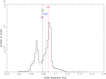
Figure 10: WMAP sky noise dispersion histogram, with the mean noise dispersion level obtained in detected deviation regions also shown. The solid histogram shown corresponds to the full sky noise dispersion map, whereas the dotted histogram corresponds to the Kp0 masked noise dispersion map. The dashed vertical lines indicate the mean noise dispersion level in the detected deviation regions illustrated in Figure 9. None of the detected deviation regions correspond to noise of higher dispersion than typical. The lettered key corresponds to the thresholded coefficient maps contained in the panels of Figure 9: (a) Mexican hat $\epsilon=0.00$, $a_{2}=100\arcmin$; (b) Mexican hat $\epsilon=0.00$, $a_{6}=300\arcmin$; (c) Mexican hat $\epsilon=0.95$, $a_{3}=150\arcmin$, $\gamma=72^{\circ}$; (d) Mexican hat $\epsilon=0.95$, $a_{10}=500\arcmin$, $\gamma=108^{\circ}$; (e) Real Morlet $\mn@boldsymbol{k}=\left(10,0\right)^{T}$, $a_{11}=550\arcmin$, $\gamma=72^{\circ}$.

5 Conclusions

A directional spherical wavelet analysis, facilitated by our fast CSWT, has been applied to the WMAP 1-year data to probe for deviations from Gaussianity. Directional spherical wavelets allow one to probe orientated structure inherent in the data. Non-Gaussianity has been detected by a number of test statistics for a range of wavelets.

We have reproduced the results obtained by Vielva et al. (2003) using the symmetric Mexican hat $\epsilon=0.00$ wavelet, thereby confirming their findings, whilst also providing a consistency check for our analysis. Deviations in the skewness and kurtosis of wavelet coefficients on scale $a_{2}=100\arcmin$ and $a_{6}=300\arcmin$ were detected, although using our more conservative test we make these detections at the 97.2% and 95.3% overall significance levels respectively (lower than the 99.9% significance level quoted by Vielva et al. (2003) for their kurtosis detection).

Similar detections of non-Gaussianity were made using the elliptical Mexican hat $\epsilon=0.95$ wavelet, although on slightly larger scales. In particular, a deviation from Gaussianity was detected in the skewness of the Mexican hat $\epsilon=0.95$ wavelet coefficients on scale $a_{3}=150\arcmin$ and orientation $\gamma=72^{\circ}$ at the 96.1% significance level. Although a detection was observed in the kurtosis outside of the 99% confidence region on scale $a_{10}=500\arcmin$ and orientation $\gamma=108^{\circ}$, the full statistical analysis of Monte Carlo simulations gave a significance of only 80.1% for this detection.

The most interesting result, however, is the deviation from Gaussianity observed in the real Morlet wavelet skewness measurement on scale $a_{11}=550\arcmin$ and orientation $\gamma=72^{\circ}$. This wavelet scale corresponds to an effective size on the sky of $\sim 26^{\circ}$ ($\sim 3^{\circ}$ for the internal structure of the real Morlet wavelet), or equivalently a spherical harmonic scale of $\ell\sim 7$ ($\ell\sim 63$). The detection deviates from the mean of 1000 Gaussian Monte Carlo simulations by $5.61$ standard deviations for the WMAP map and by $6.42$ standard deviations for the Tegmark map. Only 17 of 1000 Gaussian simulated maps exhibited a deviation this large in any real Morlet test statistic, hence the detection is conservatively made at 98.3% significance.

Significance levels were also calculated from $\chi^{2}$ tests for each spherical wavelet. This approach avoids the posterior selection of particular statistics, but rather considers the set of test statistics in aggregate. By considering the joint distribution of test statistics in this manner the analysis results may be diluted by including a large number of less powerful test statistics. Deviations from Gaussianity at significance levels of 99.9% and 99.3% were found using the symmetric Mexican hat and real Morlet wavelet respectively. In this case the directional real Morlet analysis is more severely affected by a larger number of less useful test statistics, nevertheless both deviations from Gaussianity are made at very high significance. We quote the overall significance of our findings, however, at the lower significance levels found using the previous most conservative test.

Deviations from Gaussianity corresponding to the most significant detections for each wavelet were localised on the sky. By removing the coefficients corresponding to these regions from the initial analysis, all significant non-Gaussianity detections were eliminated. These localised regions therefore appear to be the source of detected non-Gaussianity. Moreover, those regions that introduce skewness in the WMAP map may be localised, as may those regions that introduce kurtosis. Preliminary noise analysis indicates that these detected deviation regions do not correspond to regions that have higher noise dispersion than typical. Further analysis is required, however, to ascertain whether these regions correspond to the localised introduction of secondary non-Gaussianity or systematics, or whether in fact the non-Gaussianity detected in the WMAP 1-year data is due to intrinsic primordial fluctuations in the CMB.

An interesting first step in deducing whether the non-Gaussian signal discovered is of cosmological origin would be to repeat our analysis on the 4-year COBE-DMR data. Although it has been shown that these data contain some systematic effects that lead to non-Gaussianity (Magueijo & Medeiros, 2004), it is likely that these systematics are not shared by WMAP. Provided the most significant detection in the WMAP data is predominantly due to the global structure of the real Morlet wavelet at an angular scale of $\sim 26^{\circ}$, the angular resolution of the COBE-DMR data should be sufficient to observe it if it is astrophysical in origin. Clearly, it will also be of great interest to investigate whether the non-Gaussianity detections reported here are still present in the 2-year WMAP data.

Appendix A A fast directional CSWT

The CSWT at a particular scale is essentially a spherical convolution; hence it is possible to apply the fast spherical convolution algorithm proposed by Wandelt & Górski (2001) to evaluate the wavelet transform. The harmonic representation of the CSWT is first presented, followed by a discretisation and fast implementation. Without loss of generality we consider a single dilation only.

A.1 Harmonic formulation

There does not exist any finite point set on the sphere that is invariant under rotations (due to geometrical properties of the sphere), hence it is more natural, and in fact more accurate for numerical purposes, to recast the CSWT defined by (3) in harmonic space.

Both the wavelet and signal are represented in terms of a spherical harmonic expansion, defined for an arbitrary function $f\in L^{2}(S^{2})$ by

$$f(\omega)=\sum_{\ell=0}^{\infty}\sum_{m=-\ell}^{\ell}\widehat{f}_{\ell m}Y_{\ell m}(\omega)\>,$$ (17)

where the spherical harmonic coefficients are given by the usual projection of the signal onto each spherical harmonic basis function $Y_{\ell m}(\omega)$,

$$\widehat{f}_{\ell m}=\int_{S^{2}}f(\omega)\>{Y_{\ell m}}^{\ast}(\omega)\>\mathrm{\,d}\mu(\omega)\>.$$ (18)

In practice one requires that at least one of the functions, usually the wavelet, has a finite band limit so that negligible power is present in those coefficients above a certain $\ell_{\rm max}$. For all practical purposes, the outer summation of (17) may then be truncated to $\ell_{\rm max}$.

Substituting the spherical harmonic expansions of the wavelet and signal into the CSWT of (3) and noting the orthogonality of the spherical harmonics, yields the harmonic representation

$$W(\alpha,\beta,\gamma)=\sum_{\ell=0}^{\ell_{\rm max}}\>\sum_{m=-\ell}^{\ell}\>\sum_{m^{\prime}=-\ell}^{\ell}\left[{D_{mm^{\prime}}^{\ell}(\alpha,\beta,\gamma)\,\widehat{\psi}_{\ell m^{\prime}}}\right]^{\ast}\>\widehat{s}_{\ell m}.$$ (19)

The additional summation and $D_{mm^{\prime}}^{\ell}$ Wigner rotation matrices that are introduced characterise the rotation of a spherical harmonic, noting that a rotated spherical harmonic may simply be represented by a sum of rotated harmonics of the same $\ell$ by (Inui et al., 1996)

$$(\mathcal{R}_{\alpha,\beta,\gamma}Y_{\ell m})(\omega)=\sum_{m^{\prime}=-\ell}^{l}D_{mm^{\prime}}^{\ell}(\alpha,\beta,\gamma)\>Y_{\ell m^{\prime}}(\omega)\>.$$ (20)

The Wigner rotation matrices may be decomposed as

$$D_{mm^{\prime}}^{\ell}(\alpha,\beta,\gamma)=e^{-\mathit{i}m\alpha}\>d_{mm^{\prime}}^{\ell}(\beta)\>e^{-\mathit{i}m^{\prime}\gamma}\>,$$ (21)

where the real polar $d$-matrix is defined by, for example, Brink & Satchler (1993). The relationship shown in (21) is exploited by factoring the rotation $\mathcal{R}_{\alpha,\beta,\gamma}$ into two separate rotations, both of which only contain a constant $\pm\pi/2$ polar rotation:

$$\mathcal{R}_{\alpha,\beta,\gamma}=\mathcal{R}_{\alpha-\pi/2,\;-\pi/2,\;\beta}\>\>\mathcal{R}_{0,\;\pi/2,\;\gamma+\pi/2}\>.$$ (22)

By factoring the rotation in this manner and applying the decomposition described by (21), (19) can be written as

$$W(\alpha,\beta,\gamma)=\sum_{\ell=0}^{\ell_{\rm max}}\>\sum_{m=-\ell}^{\ell}\>\sum_{m^{\prime}=-\ell}^{\ell}\>\sum_{m^{\prime\prime}=-\min(m_{\rm max},\ell)}^{\min(m_{\rm max},\ell)}d_{m^{\prime}m}^{\ell}(\pi/2)\>d_{m^{\prime}m^{\prime\prime}}^{\ell}(\pi/2)$$ (23)

$$\times\>\>\widehat{\psi}_{\ell m^{\prime\prime}}{}^{\ast}\>\widehat{s}_{\ell m}\>e^{\mathit{i}[m(\alpha-\pi/2)+m^{\prime}\beta+m^{\prime\prime}(\gamma+\pi/2)]}\>,$$

where the symmetry relationship $d_{mm^{\prime}}^{\ell}(-\beta)=d_{m^{\prime}m}^{\ell}(\beta)$ has been applied. In many cases it is likely that the wavelet will have minimal azimuthal structure compared to the signal under analysis, in which case it may also have a lower effective azimuthal band limit $m_{\rm max}\ll\ell_{\rm max}$.

The harmonic formulation presented replaces the continuous integral of (3) by finite summations, although evaluating these summations directly would be no more efficient that approximating the initial integral using simple quadrature. Rotations are elegantly represented in harmonic space, however, and the approximation and interpolation required in any real space discretisation is avoided. Moreover, (23) is represented in such a way that the presence of complex exponentials may be exploited such that fast Fourier transforms (FFTs) may be applied to evaluate rapidly the three summations simultaneously.

A.2 Fast implementation

Azimuthal rotations may be applied with far less computational expense than polar rotations since they appear within complex exponentials in (23). Although the $d$-matrices can be evaluated reasonably quickly and reliably using recursion formulae (e.g. those given by Risbo 1996), the basis for the fast implementation is to avoid these polar rotations as much as possible and use FFTs to evaluate rapidly all of the azimuthal rotations simultaneously. This is the motivation for factoring the rotation by (22) so that all Euler angles occur as azimuthal rotations.

The discretisation of each Euler angle may in general be arbitrary. However, to exploit standard FFT routines uniform sampling is adopted. The uniformly sampled spherical wavelet coefficient samples are defined by

$$W_{n_{\alpha},n_{\beta},n_{\gamma}}=W\left(\frac{2\pi n_{\alpha}}{N_{\alpha}},\frac{2\pi n_{\beta}}{N_{\beta}},\frac{2\pi n_{\gamma}}{N_{\gamma}}\right)\>.$$ (24)

Discretising (23) in this manner and performing a little algebra we may recast it in a form amenable to fast Fourier techniques:

$$W_{n_{\alpha},n_{\beta},n_{\gamma}}=e^{-\mathit{i}2\pi(n_{\alpha}\ell_{\rm max}/N_{\alpha}+n_{\beta}\ell_{\rm max}/N_{\beta}+n_{\gamma}m_{\rm max}/N_{\gamma})}$$ (25)

$$\times\>\sum_{j=0}^{N_{\alpha}-1}\>\sum_{j^{\prime}=0}^{N_{\beta}-1}\>\sum_{j^{\prime\prime}=0}^{N_{\gamma}-1}t_{j,j^{\prime},j^{\prime\prime}}\>e^{\mathit{i}2\pi(jn_{\alpha}/N_{\alpha}+j^{\prime}n_{\beta}/N_{\beta}+j^{\prime\prime}n_{\gamma}/N_{\gamma})}\>,$$

where the second line is simply the unnormalised 3D inverse discrete Fourier transform (DFT) of

$$t_{m+\ell_{\rm max},m^{\prime}+\ell_{\rm max},m^{\prime\prime}+m_{\rm max}}=e^{i(m^{\prime\prime}-m)\pi/2}$$ (26)

$$\times\>\sum_{\ell=\max(\mid m\mid,\mid m^{\prime}\mid,\mid m^{\prime\prime}\mid)}^{\ell_{\rm max}}d_{m^{\prime}m}^{\ell}(\pi/2)\>d_{m^{\prime}m^{\prime\prime}}^{\ell}(\pi/2)\>\widehat{\psi}_{\ell m^{\prime\prime}}{}^{\ast}\>\widehat{s}_{\ell m}\>,$$

where the shifted indices show the conversion between the harmonic and Fourier conventions. The number of samples for each Euler angle is $N_{\alpha}=2\,\ell_{\rm max}+1$, $N_{\beta}=2\,\ell_{\rm max}+1$ and $N_{\gamma}=2\,m_{\rm max}+1$, enforced by uniform sampling and the standard Fourier relationship.

The CSWT may be performed very rapidly in spherical harmonic space by constructing the $t$-matrix of (26) from spherical harmonic coefficients and precomputed $d$-matrices, followed by the application of a FFT to evaluate rapidly all three Euler angles of the discretised CSWT simultaneously, before applying a final modulating complex exponential factor. Memory and computational requirements may be reduced by a further factor of two for real signals by exploiting the conjugate symmetry relationship $t_{-m,-m^{\prime},-m^{\prime\prime}}=t_{m,m^{\prime},m^{\prime\prime}}^{\ast}$.

The computational cost of the fast CSWT is dominated by the calculation of the $t$-matrix, which is of order $\mathcal{O}(\ell_{\rm max}^{\>3}m_{\rm max})$. A direct quadrature approximation of the CSWT integral is of order $\mathcal{O}(N_{\alpha}{}^{2}N_{\beta}{}^{2}N_{\gamma})$. The harmonic and real space size parameters are of the same order, that is $\mathcal{O}(\ell_{\rm max})\sim\mathcal{O}(N_{\alpha})\sim\mathcal{O}(N_{\beta})$ and $\mathcal{O}(m_{\rm max})\sim\mathcal{O}(N_{\gamma})$, hence the fast algorithm provides a saving of $\mathcal{O}(\ell_{\rm max})$. We give a more detailed comparison of the complexity of various CSWT implementations and typical execution times in McEwen et al. (2004).

References

- Antoine & Vandergheynst (1998) Antoine J. -P. and Vandergheynst P., 1998, Journal of Mathematical Physics, 39, 8, 3987–4008
- Antoine et al. (2002) Antoine J. -P., Demanet L., Jacques L., 2002, Applied Computational Harmonic Analysis, 13, 3, 177–200
- Barreiro & Hobson (2001) Barreiro R. B., Hobson M. P., 2001, MNRAS, 327, 813
- Barreiro et al. (2000) Barreiro R. B., Hobson M. P., Lasenby A. N., Banday A. J., Górski K. M. and Hinshaw G., 2000, MNRAS, 318, 475
- Bennett et al. (2003) Bennett C. L. et al., 2003, ApJS, 148, 97
- Brink & Satchler (1993) Brink D. M., Satchler G. R., 1993, Angular Momentum 3rd Ed., Clarendon Press, Oxford
- Cabella et al. (2004) Cabella P., Liguori M., Hansen F. K., Marinucci D., Matarrese S., Moscardini L., Vittorio N., 2004, MNRAS, submitted (astro-ph/0406026)
- Cayón et al. (2001) Cayón L., Sanz J. L., Martinez-González E., Banday A. J., Argüeso F., Gallegos J. E., Górski K. M., Hinshaw G., 2001, MNRAS, 326, 1243
- Chiang et al. (2003) Chiang L. -Y., Naselsky P. D., Verkhodanov O. V., 2003, ApJ, 590, 65
- Colley & Gott (2003) Colley W. N., Gott J. R., 2003, MNRAS, 344, 686
- Coles et al. (2004) Coles P., Dineen P., Earl J., Wright D., 2004, MNRAS, 350, 989
- (12) Copi C. J., Huterer D., Starkman G. D., 2004, Phys. Rev. D, in press (asto-ph/0310511)
- (13) Cruz M., Martinez-González E., Vielva P., Cayón L., 2004, MNRAS, in press (astro-ph/0405341)
- Eriksen et al. (2004) Eriksen, H. K., Novikov, D. I., Lilje, P. B, Banday, A. J., Górski K. M., 2004, ApJ, in press (astro-ph/0401276)
- Gaztanaga & Wagg (2003) Gaztanaga E., Wagg J., 2003, Phys. Rev. D., 68, 21302
- Górski et al. (1999) Górski K. M., Hivon E., Wandelt B. D., 1999, preprint (astro-ph/9812350)
- Hansen et al. (2004) Hansen F.K., Cabella P., Marinucci D., Vittorio N., 2004, ApJL, submitted (astro-ph/0402396)
- Hobson et al. (1999) Hobson M. P., Jones A. W., Lasenby A. N., 1999, MNRAS, 309, 125
- Inui et al. (1996) Inui T., Tanabe Y., Onodera Y., 1990, Group Theory and its Application in Physics, Springer Verlag
- Komatsu et al. (2003) Komatsu E. et al., 2003, ApJS, 148, 119
- Land & Magueijo (2004) Land K, Magueijo J., 2004, MNRAS, submitted (astro-ph/0405519)
- Larson & Wandelt (2004) Larson D. L., Wandelt B. D., 2004, ApJ, 613, 85
- McEwen et al. (2004) McEwen J. D., Hobson M. P., Lasenby A. N., Mortlock D. J., 2004, XXXIXth Rencontres de Moriond (astro-ph/0409288)
- Magueijo & Medeiros (2004) Magueijo J., Medeiros J., 2004, MNRAS, 351, L1
- Martinez-González et al. (2002) Martinez-González E., Gallegos J. E., Argüeso F., Cayón L., Sanz J. L., 2002, MNRAS, 336, 22
- Mukherjee & Wang (2004) Mukherjee P., Wang Y., 2004, ApJ, submitted (astro-ph/0402602)
- Mukherjee et al. (2000) Mukherjee P., Hobson M. P., Lasenby A. N., 2000, MNRAS, 318, 1157
- de Oliveira-Costa et al. (2004) de Oliveira-Costa A., Tegmark M., Zaldarriaga M., Hamilton A., 2004, Phys. Rev. D, 69, 63516
- Pando et al. (1998) Pando J., Valls-Gabaud D., Fang L. -Z., 1998, Phys. Rev. Lett., 81, 4568
- Risbo (1996) Risbo T., 1996, Journal of Geodesy, 70, 383
- Slosar & Seljak (2004) Slosar A., Seljak U., 2004, Phys. Rev. D, submitted, (astro-ph/0404567)
- Tegmark et al. (2003) Tegmark M., de Oliveira-Costa A., Hamilton A. J. S., 2003, Phys. Rev. D, 68, 12
- Vielva et al. (2003) Vielva P., Martinez-González E., Barreiro R. B., Sanz J. L., Cayón L., 2003, ApJ, 609, 22
- Wandelt & Górski (2001) Wandelt B. D., Górski K. M., 2001, Phys. Rev. D, 63, 123002, 1–6