Universal Non-Gaussian Velocity Distribution in Violent Gravitational Processes

Abstract

We study the velocity distribution in spherical collapses and cluster-pair collisions by use of N-body simulations. Reflecting the violent gravitational processes, the velocity distribution of the resultant quasi-stationary state generally becomes non-Gaussian. Through the strong mixing of the violent process, there appears a universal non-Gaussian velocity distribution, which is a democratic (equal-weighted) superposition of many Gaussian distributions (DT distribution). This is deeply related with the local virial equilibrium and the linear mass-temperature relation which characterize the system. We show the robustness of this distribution function against various initial conditions which leads to the violent gravitational process. The DT distribution has a positive correlation with the energy fluctuation of the system. On the other hand, the coherent motion such as the radial motion in the spherical collapse and the rotation with the angular momentum suppress the appearance of the DT distribution.

I Introduction

Galaxies and clusters of galaxies are typical structures formed through the gravity of their own. We would like to understand the history and universal characterization of these self-gravitating structures. Especially, we are interested in how extensively the formation process of them are involved in the resultant universal structure through their gravitational interaction. In these structure formation of self-gravitating systems (SGS), a cold collapse and a cluster-pair collision would be the fundamental processes. Therefore in this paper, we would like to focus on such fundamental dynamics disregarding the other non-gravity factors.

The cold collapsing process has been extensively studied as a crucial relaxation process of the collisionless systems such as elliptical galaxies where the stellar encounters are unimportant. After the violent cold collapse, a steady state is generally formed, whose density profile is well described by the de Vaucouleurs’s $r^{1/4}$ law deVaucouleurs48 ; Albada82 ; Jaffe87 ; Makino90 ; Aguilar90 . The spherical averaged density profile is found to be $\rho\propto r^{-4}$ in spherical cold collapsesHenon64 ; Albada82 and is found to be $\rho\propto r^{-3}-r^{-4}$ in the cluster-pair collision Merrall03 . The energy distribution is further discussed in Stiavelli85 . On the other hand, the velocity distribution has not yet been extensively studied except for the anisotropy of the velocity dispersionBinney87 . Recently, Merrall et al. have numerically showed that the radial velocity distribution in the central region of the bound particles becomes GaussianMerrall03 . After the spherical collapse and the cluster-pair collision, Kanaeda and Morikawa showed that the velocity distribution of all bound particles becomes non-GaussianKanaeda03 which is described by the superposed-Gaussian.

From a viewpoint of statistical mechanics, we cannot naively expect the ordinary Gaussian distributions for SGS, because the the long-range interaction of gravity apparently violates additivity, which is the basic standpoint of the ordinary Boltzmann statistical mechanicsTsallis95 . Then the question is whether we can expect any universal distribution function for SGS instead of the Gaussian distribution.

As one of the possible explanations for these non-Gaussian distributions in the stationary state with large fluctuations of intensive quantities such as temperature, Beck and CohenBeck proposed the superstatistics. According to this proposal, statistical properties of the temperature fluctuations determine overall non-Gaussian distributions. A special choice of the fluctuation leads to the Tsallis statisticsTsallis .

However, it is clear that the non-Gaussian properties of SGS are not always observed everywhere in the Universe. Moreover non-Gaussian properties of SGS are quite diverse in general and we cannot expect the completely universal properties of SGS. For example, we studied non-Gaussian properties in the self-gravitating ring modelSota01 , where many self-gravitating particles are constrained to move on a circular ring, which is fixed in the three-dimensional space. Only at the intermediate energy scale where the specific heat becomes negative, only the halo particles which belong to the intermediate energy scale, have shown non-Gaussian and power law velocity distribution: $f(v)\propto v^{-2}$. In this model, the existence of the halo particles plays an essential role in the appearance of non-Gaussian distributions. In our present paper therefore, we would like to clarify in which aspect of SGS and under which conditions the universal non-Gaussian properties are observed.

Non-Gaussian properties would be more naturally expected for the collisionless stage of the evolution ($t<t_{rel}$) than the later collisional stage of SGS ($t\gg t_{rel}$), where $t_{rel}$ is a local two-body relaxation timeSpitzer (In this paper, $t_{rel}$ is defined by Eq.(2)). This is because in the former stage, the system is not thermally relaxed and the local equilibrium is not yet established. A long range dynamical correlation among the whole system develops though the long range interaction. This property would yield non-additivity of the system and manifest deviation from the ordinary Gaussian distributions. On the other hand, in the later stage, the local equilibrium is established through two-body encounters and the situation is similar to the ordinary statistical mechanics which admits Gaussian distributions. Thus we would like to concentrate on the collisionless stage of SGS in this paper.

In section II, we begin our study with typical simulations for spherical cold collapses and cluster-pair collisions. We find the same form of non-Gaussian velocity distribution in both cases, and then we explore four different models of the superposed-Gaussian distributions to describe this velocity distribution. In section III, by analyzing the numerical data we show that the non-Gaussian velocity distribution observed in our simulation are well described by the “Democratic Temperature(DT) distribution”. This DT distribution is consistent with the fact that we observe the linear relation between the temperature and the inner mass. In section IV, we study the universality of this DT distribution and show that the mixing property under the violent gravitational process is the essence for the appearance of the DT distribution. The effect of coherent motion in the velocity distribution is discussed in section V. The last section VI is devoted to the discussions and further developments of the present work.

II the velocity distributions in N-body simulation

A self-gravitating N-body system is described by the following Hamiltonian:

$$H=\sum_{i=1}^{N}\frac{\bm{p}_{i}^{2}}{2m}-\sum_{i<j}^{N}\frac{Gm^{2}}{\left\{(\bm{r}_{i}-\bm{r}_{j})^{2}+\epsilon^{2}\right\}^{1/2}},$$ (1)

where $\bm{r}_{i}$ and $\bm{p}_{i}$ are respectively the position and the momentum of the $i$th particle, $m$ is the mass of the each particle, and $G$ is the gravitational constant. For numerical simulations, we have to introduce a cutoff parameter $\epsilon$. For the units of length, mass, and time, we use the initial system size $R$, the total mass $M:=Nm$, and the initial free fall time $t_{ff}:=\sqrt{R^{3}/(GM)}$, respectively. The local two-body relaxation time $t_{rel}$ in this simulation can be written in the following form:

$$t_{rel}=\frac{0.065\sigma^{3}(r)}{G^{2}\rho(r)m\ln(1/\epsilon)},$$ (2)

where $\sigma(r)$ is a velocity dispersion and $\rho(r)$ is a mass density. We use a leap-frog symplectic integrator on GRAPE-5, a special-purpose computer designed to accelerate N-body simulationsGRAPE . In all runs, the numerical errors in the total energy $|\Delta E/E_{0}|$ have been controlled to be less than $10^{-3}$.

In this section, we focus on the velocity distribution in the violent gravitational process by N-body simulation. Especially we consider two fundamental processes of violent gravitational dynamics; a spherical cold collapse and a cluster-pair collision.

II.1 Spherical Cold collapse process

We first glance at a typical example of a spherical cold collapse process (run SC in Table.1). All particles are homogeneously distributed within a sphere of radius $R$. The system is composed of $N=5000$ particles and we set the vanishing virial ratio $|2K/W|=0$ initially, where $K$ and $W$ are the kinetic energy and the potential energy of the whole system, respectively.

Fig.1 shows snapshots of particle distributions at different times. Most particles rapidly collapse into the center within the free-fall time $t\sim t_{ff}$. After this collapse, some particles obtain positive energy and escape from the system, and the rest particles remain bounded and gradually expand leaving a tight core at the center. This is a typical process of the formation of the core-halo structure for SGS.

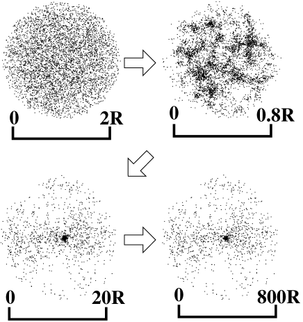
Figure 1: A snapshot of a spherical cold collapse case (run SC in Table 1): top left ($t=0$), top right ($t=1t_{ff}$), bottom left ($t=5t_{ff}$), and bottom right ($t=100t_{ff}$).

We now focus on the velocity distributions of the particles. Since we are interested in the global property, we extract the one-dimensional velocity distribution function combining all-directional components of velocity distributions. We will examine the anisotropy in the velocity distribution in Sec.V. The velocity distribution thus obtained is shown for bound particles, which have negative energy, in Fig.2. This velocity distribution is apparently different from the ordinary Gaussian distribution, especially in the small velocity region. There is an apparent cusp at the center. This velocity distribution has been stably observed just after the collapse during the whole simulation time ($t\sim t_{ff}\rightarrow 1000t_{ff}$). We emphasize that this non-Gaussian velocity distribution is quite universal and robust in various cold collapsing process, as we will demonstrate briefly.

Figure 2: A velocity distribution of a spherical cold collapse (run SC in Table 1) at $t=10t_{ff}$. Three best-fitted Gaussian distributions are superposed. Gauss (all) is fitted by use of the all data. Gauss (small) and Gauss (large) are fitted by use of data included for only small velocity and only large velocity, respectively.

II.2 Cluster-pair collision process

We turn our attention to another case of the violent gravitational process: The cluster-pair collision. Because we would like to clarify the basic process, we choose the simplest head-on collision (run CC in Table.2). Each cluster has an equal number of particles and all particles are homogeneously distributed in each sphere of radius $R$. The initial velocity distribution is set to be Gaussian and the initial virial ratio is $1$. We set the initial separation of the pair to $6R$ along the $x$ axis.

Fig.3 shows the snapshots of particle distributions for the run CC at different times. The cluster-pair collides at time $t\sim 20t_{ff}$ and then gradually merges into a single cluster. The velocity distribution profile after this merging is shown in Fig.4. The velocity distribution profile is very similar to the previous spherical collapse case(run SC). The excess of velocity distribution at the small value is prominent as before.

In both cases, we notice that the temperature or the velocity dispersion is different from place to place; the center of the core is much hotter than the outskirts of the system. Therefore it is clear from the beginning that the obtained velocity distribution cannot be fitted by a single Gaussian distribution. Thus we propose to describe these systems by the superposition of Gaussian distributions with various temperatures. This consideration is very natural because the collisionless SGS allows the coexistence of many temperatures. This is because (a) the collisionless SGS is not yet thermally relaxed, and (b) the virial relation implies that the system shows negative specific heat, which spontaneously yields inhomogeneous temperature.

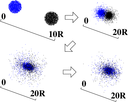
Figure 3: A snapshot of a cluster collision model (run CC in Table 2): top left ($t=0$), top right ($t=5t_{ff}$), bottom left ($t=20t_{ff}$), and bottom right ($t=500t_{ff}$).

Figure 4: Same as Fig.2, but for a cluster-pair collision model (run CC in Table 2) at $t=500t_{ff}$.

In general, superposition of Gaussian velocity distribution $f_{SG}(v_{i})$ has the form:

$$f_{SG}(v_{i}) = A\int_{0}^{M}dM^{\prime}\frac{1}{\sqrt{2\pi T(M^{\prime})}}e^{-v_{i}^{2}/2T(M^{\prime})},$$ (3)

$$= A\int_{0}^{T}dT^{\prime}\left|\frac{dM}{dT^{\prime}}\right|\frac{1}{\sqrt{2\pi T^{\prime}}}e^{-v_{i}^{2}/2T^{\prime}},$$

where $A$ is a normalization constant. The parameter function $M$ can be any function of temperature. However now in the present spherical symmetric case, we can choose it to be the inner mass: $M_{r}:=\int_{0}^{r}\rho\left(r^{\prime}\right)4\pi r^{\prime 2}dr^{\prime}$. This choice is not at all trivial and will be demonstrated briefly. Any special choice of the weight function for the superposition yields in general arbitrary distribution functions. In order to avoid such arbitrariness, we will choose the simplest weight functions. Here we consider four natural models of the superposed-Gaussian distribution.

• Model 1 (GT) Gaussian-weighted superposition of Gaussian distributions with various temperatures.

  The temperature distribution is the Gaussian with the dispersion $\tau$, and GT distribution $f_{GT}(v_{i},\tau)$ takes the following form:

  $$f_{GT}(v_{i},\tau) = \int_{0}^{\infty}dT\frac{1}{\sqrt{2\pi\tau}}\exp\left[-\frac{T^{2}}{2\tau}\right]\frac{1}{\sqrt{2\pi T}}\exp\left[-\frac{v_{i}^{2}}{2T}\right]$$ (4)

  $$= \frac{1}{2\pi\sqrt{\tau}}\left[\frac{\tau^{1/4}\Gamma(1/4){}_{0}F_{2}(1/2,3/4;-v_{i}^{4}/(32\pi))}{2^{3/4}}\right.$$

  $$\left.-\sqrt{2\pi}|v_{i}|{}_{0}F_{2}(3/4,5/4;-v_{i}^{4}/(32\tau))\right.$$

  $$\left.+\frac{v_{i}^{2}\Gamma(3/4){}_{0}F_{2}(5/4,3/2;-v_{i}^{4}/(32\pi))}{2^{1/4}\tau^{1/4}}\right],$$

  where $\Gamma(x)$ is a Gamma function and ${}_{p}F_{q}(\alpha_{1},\dots,\alpha_{p};\beta_{1},\dots,\beta_{q};z)$ is the generalized Hypergeometric function.

• Model 2 (DT) Equal-weighted superposition of Gaussian distributions with various temperatures.

  This case corresponds to $dT/dM=const.$ in terms of the parameter function $M$, and we call the velocity distribution in this case as “democratic temperature distribution”$f_{DT}(v_{i})$:

  $$f_{DT}(v_{i}) = \frac{1}{T}\int_{0}^{T}{dT^{\prime}\frac{1}{\sqrt{2\pi T^{\prime}}}e^{-v_{i}^{2}/\left(2T^{\prime}\right)}},$$

  $$= \frac{1}{T}\left[{\sqrt{\frac{2T}{\pi}}e^{-v_{i}^{2}/(2T)}-\left|{v_{i}}\right|\left\{{1-\mbox{Erf}\left({\frac{\left|{v_{i}}\right|}{\sqrt{2T}}}\right)}\right\}}\right],$$

  where $\mbox{Erf}(x)$ is the error function:

  $$\mbox{Erf}(x):=\frac{2}{\sqrt{\pi}}\int_{0}^{x}dte^{-t^{2}}.$$

• Model 3 (G$\sigma$ ) Gaussian-weighted superposition of Gaussian distributions with various standard deviations $\sigma:=\sqrt{T}$.

  The distribution of the standard deviation is the Gaussian with the dispersion $\gamma^{2}$, and G$\sigma$ distribution $f_{G\sigma}(v_{i},\gamma)$ takes the following form:

  $$f_{G\sigma}(v_{i},\gamma) = \int_{0}^{\infty}d\sigma\frac{1}{\sqrt{2\pi}\gamma}\exp\left[-\frac{\sigma^{2}}{2\gamma^{2}}\right]\frac{1}{\sqrt{2\pi}\sigma}\exp\left[-\frac{v_{i}^{2}}{2\sigma^{2}}\right],$$ (6)

  $$= \frac{K_{0}\left(\left|{v_{i}/\gamma}\right|\right)}{2\pi\gamma},$$

  where $K_{0}(z)$ is the modified Bessel function.

• Model 4 (D$\sigma$ ) Equal-weighted superposition of Gaussian distributions with various standard deviation $\sigma$.

  Since $d\sigma/dM=const.$, D$\sigma$ distribution $f_{D\sigma}(v_{i})$ has the following form:

  $$f_{D\sigma}(v_{i}) = \frac{1}{\sigma}\int_{0}^{\sigma}d\sigma^{\prime}\frac{1}{\sqrt{2\pi}\sigma^{\prime}}e^{-v_{i}^{2}/\left(2\sigma^{\prime 2}\right)},$$ (7)

  $$= \frac{\Gamma(0,v_{i}^{2}/\left({2\sigma^{2}}\right))}{2\sqrt{2\pi}\sigma},$$

  where $\Gamma(z,p)$ is the incomplete Gamma function.

In the next section, we examine the above four models in relation with our non-Gaussian velocity distributions.

III Democratic Temperature (DT) distribution

As shown in the preceding section, the velocity distribution functions for both processes, spherical cold collapses and cluster-pair collisions, take the same non-Gaussian form. Using the most natural four models of superposed-Gaussian distributions, we try to fit our velocity distribution function and to extract any universal character of SGS.

Figure 5: A linear-log plot for velocity distribution for the case of a spherical cold collapse (run SC) at $t=10t_{ff}$. The best fit Gaussian and the four superposed-Gaussian model (Eqs.(4),(LABEL:DT),(6), and (7)) with a best fit parameter are superposed. The $\chi^{2}$ of each model is 0.00095(Gauss), 0.00037(DT), 0.00048(GT), 0.0016(D$\sigma$), and 0.0025(G$\sigma$). The best fit model is a DT distribution.

Figure 6: Same as Fig.5, but for a cluster-pair collision model (run CC) at $t=500t_{ff}$. The $\chi^{2}$ of each model is 0.0030(Gauss), 0.0021(DT), 0.0030(GT), 0.010(D$\sigma$), and 0.015(G$\sigma$). The best fit model is a DT distribution.

The fitting results are shown in Fig.5 and 6. Using the $\chi^{2}$ analysis, the best fit model turns out to be the DT distribution in both cases.

In order to investigate the structure of velocity space for bound particles in detail, we divide the whole particles into several shells with equal number of particles. We introduce the inner mass coordinate $M_{r}:=4\pi\int_{0}^{r}dr^{\prime}r^{\prime 2}\rho(r^{\prime})$ and consider the averaged quantities within each shell as local variables.

Figure 7: A linear-log plot for a velocity distribution of each shell for the case of a spherical cold collapse (run SC). We divided the whole bound particles into 10 shells including an equal mass and calculated the velocity distribution by use of the data from $t=10t_{ff}$ and $t=20t_{ff}$.

Figure 8: Same as Fig.7, but for a cluster-pair collision (run CC). We calculated the velocity distribution by use of the data from $t=500t_{ff}$ and $t=510t_{ff}$.

The velocity distribution of each shell shows almost Gaussian (Fig.7 and 8). These figures show that each shell has a different temperature and suggest that the previous non-Gaussian distribution can be described by the superposition of Gaussians with various temperatures. The temperature is the highest at the most inner shell and monotonically decreases toward outside shells.

Figure 9: A mass dependence of velocity dispersion ($<v^{2}(M_{r})>$) for the case of a spherical cold collapse (run SC). The mass is normalized by the mass of whole bound particles $M_{b}$. The velocity dispersion is time averaged and the error bar is calculated from the time fluctuation.

Figure 10: Same as Fig.9, but for a cluster-pair collision (run CC).

The local velocity dispersion $<v^{2}>$ is plotted against the inner mass $M_{r}$ in Fig.9 and 10. In both cases, it is remarkable that the velocity dispersion decreases linearly in the inner mass $M_{r}$. We emphasize here that this linear relation is quite robust and universal. Actually this relation is observed in our two processes with wide range class of initial conditions, which will be further discussed in the subsequent sections. If we carefully look at Fig.9, the temperature gradient in the inner region gradually reduces in time, while it remains constant in the outer region. Since the mass density at the inner region increases in time and eventually the effect of two-body relaxation turns on, such a tilt of the temperature gradient is thought to be caused by this collisional effect. A careful check of our numerical simulation supports this interpretation. Therefore the linearity of the temperature gradient is thought to be the property of the collisionless SGS. Further collisional effect would eventually yield the uniform temperature distributions.

The almost Gaussian velocity distribution in each shell guarantees the form of Eq.(3) and the linearity of the temperature-mass relation leads to the relation $|dM/dT|=const.$ in Eq.(3), which indicates the DT distribution for the velocity distributions. This is perfectly consistent with the result that the DT distribution is the best fit to the velocity distribution among several models which we examined.

Besides this linearity in the diagram of the local velocity dispersion $<v^{2}>$ and the inner mass $M_{r}$, we observe another prominent fact that the virial relation between the potential energy and kinetic energy holds locally at each spatial region. Using the local kinetic energy $K_{r}$ and the local potential energy $W_{r}$ inside the radius $r$, we can locally define the virial ratio $|2K_{r}/W_{r}|$. The time evolution of this local virial ratio is depicted in Fig.11 and 12. The value of the local virial ratio stays almost unity within the error $\pm 10\%$ everywhere anytime. This suggests that not only the whole system but also each shell is locally virialized. This fact may be deeply related with the robustness of the DT distribution, and will be separately discussed in Sota04 .

Figure 11: The local virial relation for run SC. The ratio $\left|2\overline{K}_{r}/\overline{W}_{r}\right|$ is plotted as a function of $M_{r}$. The virial ratios of each shell at different times ($t=5t_{ff}$, $10t_{ff}$, $50t_{ff}$, and $100t_{ff}$) are superposed.

Figure 12: Same as Fig.11, but for a cluster-pair collision (run CC). The virial ratios of each shell at different times ($t=100t_{ff}$, $200t_{ff}$, $500t_{ff}$, and $1000t_{ff}$) are superposed.

In order to examine the stability of DT distribution, we calculate the time evolution of the $\chi^{2}$ value for DT ($\chi_{DT}^{2}$) and Gaussian distributions ($\chi_{Gauss}^{2}$), which is depicted in Fig.13 and 14. Immediately after the collapse or the merging, the velocity distribution always becomes the DT distribution during the whole period of our simulations. This robustness makes DT distribution one of the most characteristic properties of collisionless SGS.

Figure 13: Time evolution of $\chi^{2}_{DT}$ of DT distribution and $\chi^{2}_{Gauss}$ of Gaussian for the case of a spherical cold collapse (run SC).

Figure 14: Same as Fig.13, but for a cluster-pair collision (run CC).

IV Universality of DT distribution - degree of violence

As we have seen in the preceding section, DT distribution, supported from the linear $<v^{2}>$ - $M_{r}$ relation, is one of the most relevant characteristics of SGS such as the spherical cold collapses and cluster-pair collisions. We would like to further clarify the condition for the appearance of the DT distribution function. From the beginning of our numerical experiments, we have implicitly chosen the violent processes such as cold collapse and the quiet cluster-pair collision. We had in mind the expectation that the strong mixing property associated with the violent gravitational process would yield the most prominent characteristics for the collisionless SGS. Actually it is well known that a violent mixing becomes an important factor to realize the quasi-equilibrium virialized stateLynden67 .

In this section, we will quantitatively demonstrate this expectation. Especially we would like to explore the correlation between the DT distribution and the degree of violence of the processes.

We control the degree of violence of the process by the choice of initial conditions in our numerical experiments. The initial conditions of all runs are listed in Table.1 for spherical collapses and Table.2 for cluster-pair collisions.

Table 1: Initial condition for spherical collapse case. $N$ is a number of particles and $|2K/W|$ is an initial virial ratio and $\rho\propto r^{-a}$ is an initial density profile and $\epsilon$ is a cutoff parameter in Eq.(1).

run	N	$|2K/W|$	$\rho\propto r^{-a}$	$\epsilon$
SC	5000	0	0	$2^{-8}$
SCN1	10000	0	0	$2^{-8}$
SCN2	50000	0	0	$2^{-8}$
SCV1	5000	0.1	0	$2^{-8}$
SCV2	5000	0.2	0	$2^{-8}$
SCV3	5000	0.3	0	$2^{-8}$
SCV4	5000	0.4	0	$2^{-8}$
SCV5	5000	0.5	0	$2^{-8}$
SCV6	5000	1.0	0	$2^{-8}$
SCA1	5000	0	0.5	$2^{-8}$
SCA2	5000	0	1.0	$2^{-8}$
SCA3	5000	0	1.5	$2^{-8}$
SCA4	5000	0	2.0	$2^{-8}$
SCC1	5000	0	0	$2^{-4}$
SCC2	5000	0	0	$2^{-6}$
SCC3	5000	0	0	$2^{-10}$
SCS1	5000	0.1	0	$2^{-8}$
SCS2	5000	0.5	0	$2^{-8}$
SCS3	5000	1.0	0	$2^{-8}$

Table 2: Initial condition for cluster collision case. $N$ is the total number of particles and the number of particles in each cluster is $N/2$. $|2K/W|$ is an initial virial ratio of each cluster where the kinetic energy $K$ is contributed by only the random motion. $K_{rot}$ is a kinetic energy by only the rotation with an orbital angular moment around the z axis ($L_{z}$) initially.

run	$N$	$|2K/W|$	$|2K_{rot}/W|(L_{z})$
CC	5000	1	0
CCL1	5000	1	0.1
CCL2	5000	1	0.2

As the indicator for the degree of violence of the process, we use the total energy fluctuation of particles; more violent the process the more rapid the energy mixing of each particles. More precisely, the energy fluctuation of the $i$th particle is defined as

$$\sigma_{e;i}:=\sqrt{\overline{e_{i}^{2}(t)}-\overline{e_{i}(t)}^{2}},$$ (8)

where $e_{i}(t)$ is the energy of $i$th particle at time $t$ and $\overline{\ast}$ is the time averaged value of $\ast$ during the whole simulation period. Then we define the total energy fluctuation of the system as the sum of $\sigma_{e;i}$ for all particles as

$$\sqrt{\Delta E^{2}}:=\sum_{i=1}^{N}\sigma_{e;i}.$$ (9)

In order to check the efficiency of $\sqrt{\Delta E^{2}}$ as the indicator of the degree of violence, we calculate the correlations with other physical quantities which are naturally expected to be connected with the strength of the mixing. When violent mixing in the phase space occurs, some of the particles obtain enough energy to escape from the system through the energy exchange by the potential oscillation. Then the rest of the particles becomes more tightly bounded due to the extraction of energy by the escaping particles. Therefore both (a) the system size and (b) the total energy of the bound particles, $E_{b}(<0)$, will become smaller after the collapse, provided the mixing is strong and effective. As the quantitative indicator for (a), i.e., the size of the system after the collapse, we introduce the half-mass radius divided by it’s initial value: $R_{hm}$. Further, we need to take ensemble average $<\ast>$ of all those quantities for the regular continuous indicator for the process.

Figure 15: The half-mass radius normalized by it’s initial value at $t=0$, $R_{hm}$ and the absolute value of the total energy of bound particles, $|E_{b}|$ are plotted against $\sqrt{\Delta E^{2}}$ for all cases in Table.1 and Table.2. We take the ensemble average for each data with several times. It ranges from $t=10t_{ff}$ to $t=100t_{ff}$ with $10t_{ff}$ intervals in the spherical case, and from $t=100t_{ff}$ and $t=1000t_{ff}$ with $100t_{ff}$ intervals in cluster collisions. The error bar is calculated from the ensemble average.

Figure 16: $\chi^{2}_{DT}/\chi^{2}_{Gauss}$ for all cases in Table.1 and Table.2. $\chi^{2}$ is a time averaged from $t=10t_{ff}$ and $t={100t_{ff}}$ at $10t_{ff}$ intervals for the spherical collapse case, from $t=100t_{ff}$ and $t={1000t_{ff}}$ at $100t_{ff}$ intervals for the cluster collision case. The error bar is calculated from the time fluctuation.

Figure 17: Same as Fig.16, but for $\chi^{2}_{DT}$.

As in shown in Fig.15, $<\sqrt{\Delta E^{2}}>$ is apparently correlated with both $<R_{hm}>$ and $<E_{b}>$. This fact supports that the total energy fluctuation $<\sqrt{\Delta E^{2}}>$ is actually an effective indicator of the degree of strength of the mixing.

Keeping in mind that $<\sqrt{\Delta E^{2}}>$ is a good indicator of the violence of the process, we now examine the correlation between the degree of violence in the initial stage and the occurrence of the DT distribution for bound particles in the quasi-equilibrium stage. We calculated $\chi^{2}$ values for the fitting of velocity distributions with DT distribution and Gaussian distribution for all runs. The result is shown in Fig.16, where the ratio of $\chi_{DT}^{2}$ of DT distribution to $\chi_{Gauss}^{2}$ of Gaussian distribution is plotted against $<\sqrt{\Delta E^{2}}>$ for all initial conditions. The value is greater than one for the simulations with small value of $<\sqrt{\Delta E^{2}}>$, which means that the velocity distribution is better fitted by Gaussian rather than DT distribution. On the other hand, for the larger values of $<\sqrt{\Delta E^{2}}>$, the data is better fitted by DT distribution rather than Gaussian. Thus DT velocity distribution is always favorable in the simulation with violent processes.

This point is further clarified in Fig.17, where we plotted the value of $\chi_{DT}^{2}$ against $<\sqrt{\Delta E^{2}}>$. It is apparent that the $\chi_{DT}^{2}$ monotonically decreases for increasing $\sqrt{\Delta E^{2}}$. These results manifestly support our expectation that the DT velocity distribution is associated with the strength of the violent mixing.

From these results, we can claim that the DT velocity distribution function is universal for various initial conditions provided that the violent gravitational process is included. Moreover, the DT distribution becomes more prominent for stronger violent processes.

V Universality of DT distribution - degree of coherence

We have so far studied the universality of DT distribution and its correlation with the degree of violence of the dynamical process. Here in this section, we further discuss another aspect of universality of DT distribution function.

In the above argument, we have neglected possible anisotropy in the velocity space; we have extracted one dimensional velocity data set by simply combining all the velocity components. However actually in the processes of spherical collapse and cluster-pair collision, the velocity space is anisotropic in general. Further the anisotropy in the rotating collapse (runs SCS1-3 in Table1) is apparent.

For example, we first consider the spherical cold collapse (run SC). Fig.18 shows the measure of validity of DT distribution, i.e., the time evolution of $\chi_{DT}^{2}$ divided by $\chi_{Gauss}^{2}$. The radial velocity distribution is better fitted by Gaussian for a while until $t\sim 50t_{ff}$ and after that time DT distribution becomes better. On the other hand, the tangential velocity distribution is always well fitted by DT distribution during all our simulation period.

This behavior will be related with the coherent motion of the particles. More precisely, in the early stage of the evolution, there exists a coherent radial motion such as a collapse and a subsequent bounce, which eventually decays. This coherent motion does not affect the tangential velocity distribution. Moreover this coherent motion may inherit some amounts of randomness in the initial distribution of particles. Therefore in the early stage, only the radial velocity component is dominated by the coherent motion with this initial spatially random distribution, and eventually recovers the intrinsic DT distribution when the coherent motion decays.

The above consideration is also applicable for the anisotropy in the rotating collapse (runs SCS1-3 in Table1). Fig.19 shows the measure of validity of DT distribution, i.e., the time evolution of $\chi_{DT}^{2}$ divided by $\chi_{gauss}^{2}$ in this case. Only the $v_{z}$-component shows DT distribution all the time, and the $v_{x},v_{y}$-components, the direction of coherent rotation, never show DT distribution during our simulation time.

Therefore the condition for the appearance of the universal DT distribution would be, besides the violence of the system, the decay of the coherent motion, which keeps the information of initial conditions.

Figure 18: Time evolution of $\chi_{DT}^{2}$ of DT distribution divided by the $\chi_{Gauss}^{2}$ for the case of a spherical cold collapse (run SC).

Figure 19: Same as Fig.18, but for the case of a spherical collapse with the angular momentum $L_{z}$ (run SCS2).

VI Conclusions and Discussions

We have studied the velocity distribution function of self-gravitating systems (SGS) which experienced violent gravitational processes by use of N-body simulation method. Especially we have chosen two fundamental processes which mimic the galaxy formation dynamics; the spherical cold collapse and the cluster-pair collision.

In both cases, after the collapses or the collisions, all the bound particles form a single stationary state, which are characterized by the local virial relation and the linearity in the mass-temperature relation. In this stationary state, the velocity distribution is well described by the democratic (=equally weighted) superposition of Gaussian distributions of various temperatures (DT distribution).

This DT velocity distribution is robust against various initial conditions such as the change of the particle number, the virial ratio, and the density profile. Moreover, using the half-mass radius and the root mean square of energy variation as a measure of the degree of violent mixing, we found a firm positive correlation between the DT distribution and the degree of violent mixing. This correlation suggests that the DT distribution originates from a violent mixing in SGS.

Carefully examining the anisotropy in the velocity distributions, we have also found another condition for the appearance of DT distributions. If any systematic coherent motion exists then it could inherit special initial condition and could suppress any intrinsic properties such as DT distribution for SGS. This coherent motion actually exists in the radial velocity distribution in the spherical collapse processes, and in the rotational velocity distribution in the processes with non-vanishing angular momentum.

As a conclusion, we postulate that both the local virial relation and DT velocity distribution, associated with the linear temperature-mass relation, are universal properties of SGS which undergo violent gravitational mixing.

The origin of the above universal properties should be further investigated. One possible candidate would be a steady heat flow from the center toward outskirts of the spherical system. In our calculation, the two-body relaxation process is initiated at the very center of the core region, within our numerical calculation period. Release of the gravitational energy at the center would yield a steady heat flow toward the outskirts of the system. This flow may guarantee the two properties we found in this paper and their duration. We hope we can report the detail very soon.

In this paper, we paid attention only to the velocity distribution function. However, we need the information of matter configuration like density profile to understand the full characteristic of gravitationally bound systems in quasi-equilibrium state. We will show that the combination of the local virial condition and the linear mass-temperature relation leads to a universal density profile for gravitationally bound systems in a separate report Sota04 . This information should give a hint for the origin of the universality profile of dark matter or elliptical galaxies like de Vaucouleurs law deVaucouleurs48 .

In our previous workSota01 , we have studied the self-gravitating ring model and have obtained a non-Gaussian velocity distribution. This velocity distribution shows a power law and is apparently different from the results obtained in this paper. We believe that this discrepancy originates from the difference of the boundary conditions. In the self-gravitating ring model, the configuration space is compact. On the other hand, in the present simulation, the configuration space is open. We would like to extensively consider the effect of boundary conditions soon.

In this work, we restricted our models only to the spherical collapses and the cluster-pair collisions. However actual galaxies may undergo much more diverse evolution processes including chemical evolution, the environment effects, and a possible special nature of the cold dark matter. So the actual observational possibility of the universality we found for astronomical objects should be further investigated.

- (1) G. de Vaucouleurs, Ann. Astrophys. 11, 247 (1948).
- (2) T. S. van Albada, Mon. Not. R. Astron. Soc. 201, 939 (1982).
- (3) W. Jaffe, Structure and Dynamics of Elliptical Galaxies, I. A. U. Symp. 127, ed. T. de Zeeuw (D. Reidel, Dordrecht), p.511 (1987).
- (4) J. Makino, K. Akiyama, and D. Sugimoto, Publ. Astron. Soc. Japan 42, 205 (1990).
- (5) L. A. Aguilar and D. Merritt, Astrophys. J. 354, 33 (1990).
- (6) M. Hénon, Ann. Astrophys. 27, 83 (1964).
- (7) T. E. C. Merrall and R. N. Henriksen, Astrophys. J. 595, 43 (2003).
- (8) M. Stiavelli and G. Bertin, Mon. Not. R. Astron. Soc. 217, 735 (1985).
- (9) N. Kanaeda and M. Morikawa, Natural Science Report of the Ochanomizu University 54, 19 (2003).
- (10) J. Binney and S. Tremaine, Galactic Dynamics (Princeton University Press, Princeton, 1987).
- (11) P. Jund, S.G. Kim, and C. Tsallis, Phys. Rev. B 52 (1995), 50.
- (12) C. Beck and E. D. G. Cohen, Physica A 322, 267 (2003).
- (13) C. Tsallis, J. Stat. Phys. 52, 479 (1988).
- (14) Y. Sota, O. Iguchi, M. Morikawa, T. Tatekawa, and K. Maeda, Phys. Rev. E 64, 056133 (2001).
- (15) L. Spitzer, Jr., Dynamical evolution of globular clusters (Princeton University Press, Princeton, 1987).
- (16) A. Kawai, T. Fukushige, J. Makino, and M. Taiji, Publ. Astron. Soc. Japan 52, 659 (2000).
- (17) L. Bell, Mon. Not. R. Astron. Soc 136, 101 (1967).
- (18) Y. Sota, O. Iguchi, M. Morikawa, and A. Nakamichi, astro-ph/0403411, submitted to Phys. Rev. Lett, (2004).