SDSS galaxy bias from halo mass-bias relation and its cosmological implications

Abstract

We combine the measurements of luminosity dependence of bias with the luminosity dependent weak lensing analysis of dark matter around galaxies to derive the galaxy bias and constrain amplitude of mass fluctuations. We take advantage of theoretical and simulation predictions that predict that while halo bias is rapidly increasing with mass for high masses, it is nearly constant in low mass halos. We use a new weak lensing analysis around the same SDSS galaxies to determine their halo mass probability distribution. We use these halo mass probability distributions to predict the bias for each luminosity subsample. Galaxies below $L_{*}$ are antibiased with $b<1$ and for these galaxies bias is only weakly dependent on luminosity. In contrast, for galaxies above $L_{*}$ bias is rapidly increasing with luminosity. These observations are in an excellent agreement with theoretical predictions based on weak lensing halo mass determination combined with halo bias-mass relations. We find that for standard cosmological parameters theoretical predictions are able to explain the observed luminosity dependence of bias over 6 magnitudes in absolute luminosity. We combine the bias constraints with those from the WMAP and the SDSS power spectrum analysis to derive new constraints on bias and $\sigma_{8}$. For the most general parameter space that includes running and neutrino mass we find $\sigma_{8}=0.88\pm 0.06$ and $b_{*}=0.99\pm 0.07$. In the context of spatially flat models we improve the limit on the neutrino mass for the case of 3 degenerate families from $m_{\nu}<0.6$eV without bias to $m_{\nu}<0.18$eV with bias (95% c.l.), which is weakened to $m_{\nu}<0.24$eV if running is allowed. The corresponding limit for 3 massless + 1 massive neutrino is 1.37eV.

I Introduction

Galaxy clustering has long been recognized as a powerful tool to constrain cosmology. Galaxies are assumed to trace dark matter on large scales and so the galaxy power spectrum can be related to that of the dark matter. The latter depends on several cosmological parameters, such as the epoch of matter-radiation equality, baryon to dark matter ratio and the primordial power spectrum shape and amplitude. The key assumption underlying this approach is that galaxies trace dark matter up to an overall factor, called the linear bias $b$, so that the galaxy and matter power spectra are related as $P_{\delta_{\rm g}}(k)=b^{2}P_{\delta_{\rm dm}}(k)$, where $\delta_{\rm g}$ and $\delta_{\rm dm}$ are the galaxy and dark matter density fluctuations, respectively, and $P(k)$ is their power spectrum.

The linear bias assumption is thought to be accurate on large scales, but becomes less and less accurate on small scales, where details of galaxy formation play an important role. The exact transition scale between the linear and nonlinear regimes does not have to equal that of dark matter and may depend on the type of galaxies one is observing, the treatment of redshift space distortions and the cosmological model. For normal galaxies it is believed to be somewhere around $k=0.1-0.2h/{\rm Mpc}$ (Hatton and Cole, 1998; Scoccimarro et al., 2001; Seljak, 2001).

While the shape of the galaxy power spectrum for $k<0.2h/{\rm Mpc}$ has been used to constrain the cosmological parameters (Percival et al., 2002; Tegmark et al., 2003a), the overall amplitude is often ignored. The reason for this is that the galaxies can be biased relative to the dark matter and the bias parameter $b$ depends on the galaxy properties, such as luminosity or type. This has long been observed as a function of morphological type (Davis and Geller, 1976). More recent surveys emphasized the luminosity dependence of bias, finding that brighter galaxies cluster more strongly both in 2dF (Norberg et al., 2001) and in SDSS (Zehavi et al., 2002). These early studies focused on the nonlinear or quasi-linear scales below 10$h^{-1}$Mpc, so it was not clear that their conclusions applied to the linear regime. In particular, on small scales the clustering strength can increase as a function of luminosity if the brighter galaxies preferentially populate larger halos with many galaxies inside, such as groups and clusters. In this case the increase in clustering amplitude on small scales is a reflection of the enhanced correlations inside the halo and is not necessarily a reflection of these halos being more correlated among themselves. In contrast with these previous studies a recent analysis of SDSS galaxy survey data has focused the analysis on $k<0.2h$/Mpc (scales above 10$h^{-1}$Mpc) and thus measured the linear bias directly (Tegmark et al., 2003b). This analysis also found that bias increases as a function of luminosity, in a similar way as in the previous studies (Norberg et al., 2001; Zehavi et al., 2002). The relative amplitudes of fluctuation power spectra for different luminosity subsamples was found to differ by almost a factor of 2.5 from the bright to the faint end. It appears therefore that the evidence for linear bias increasing with luminosity has finally been established. In this situation it is not clear which of the galaxies are unbiased ($b=1$). In the absence of additional information the overall amplitude of galaxy fluctuations thus cannot be directly related to that of dark matter.

There are at least three ways that have been proposed so far to break the degeneracy. One is to use redshift space distortions, which on large scales depend on the parameter $\beta=\Omega_{m}^{0.6}/b$, where $\Omega_{m}$ is the matter density of the universe. Unfortunately, even with modern surveys such as 2dF and SDSS, this parameter has considerable statistical uncertainty, so in itself this method cannot give a sufficiently precise bias determination. For example, the SDSS analysis gives $\beta=0.5\pm 0.2$ on scales where nonlinear redshift space distortion modeling is reliable (Tegmark et al., 2003b).

A second approach is to determine the bias from the bispectrum, as was done for 2dF galaxies (Verde et al., 2002). It is difficult to measure the bispectrum on very large scales, where deviations from nongaussianity are small. In Verde et al. (2002) most of the weight comes from scales with $0.2h/{\rm Mpc}<k<0.3h/$Mpc, in which case however it is not obvious that the bias measured there also applies to the larger scales where the power spectrum is measured, given how rapidly the nonlinear effects become important. In principle one could verify this with simulations, but pure N-body simulations (used so far) are not sufficient to verify this hypothesis, since galaxies do not trace dark matter on small scales and the details of how galaxies populate halos change the two and three point functions and depend on the specifics of the particular galaxy formation model.

A third approach is to compare a weak lensing power spectrum determination, tracing dark matter, to the galaxy power spectrum or the weak lensing-galaxy cross-correlation. This approach can also give the bias directly, but is limited by the statistical power of weak lensing measurements. These are currently significantly more noisy than those of galaxies, since on large scales the weak lensing signal is weak and the survey areas probed so far are small. Current data sets have not yet reached the scales where linear theory is valid (Hoekstra et al., 2002; Sheldon et al., 2003). In addition, shear calibration and background galaxy redshift distribution errors remain and may lead to errors as large as 20% on the linear amplitude Hirata et al. (2004). Finally, so far these studies have averaged over galaxies covering a broad range of luminosity over which the bias changes significantly, in which case comparing galaxy auto-correlation with galaxy-dark matter cross-correlation overestimates the bias even on linear scales, since $\langle b^{2}\rangle/\langle b\rangle>\langle b\rangle$ (where $\langle\rangle$ denotes averaging over luminosity).

Given the difficulties of the methods described above, most workers adopt the conservative approach and ignore the overall amplitude of fluctuations (i.e., marginalize over a completely unconstrained bias factor when deriving constraints on other parameters). Alternatively one can use other methods to determine the amplitude, such as the cluster abundance or weak lensing. These methods have systematics of their own, and at present various estimates of $\sigma_{8}$ vary by up to 30-40% (see Tegmark et al. (2003a) for a recent overview of current results). It would be useful to improve upon this situation, as the overall amplitude of fluctuations at zero redshift is an important source of information. It is especially useful to constrain the dark energy equation of state and neutrino mass.

The purpose of this paper is to propose a new approach to determine the bias parameter and to apply it to SDSS data. The main element of the method is to relate the observed luminosity bias to ab initio predictions of the halo-to-mass bias relation. The relation between bias and halo mass is one of the fundamental predictions of large scale structure models (Cole and Kaiser, 1989; Mo and White, 1996; Sheth and Tormen, 1999; Sheth et al., 2001). The bias predictions depend on the cosmological model, in particular on the nonlinear halo mass (defined below) where the bias is unity. Above this mass the bias is rapidly increasing with halo mass. Below this mass the bias is slowly decreasing to a value $b\sim 0.7$, independent of the other cosmological parameters (Jing, 1998; Sheth et al., 2001; Seljak and Warren, 2004). If one determines observationally the bias as a function of halo mass one can compare it to theoretical predictions to establish the viability of this model. This is particularly simple if one observes directly the low mass plateau, since one can then determine the absolute bias even without accurate halo mass determinations.

If we determine the correlations of dark matter halos as a function of their mass we also determine the overall amplitude of fluctuations. However, we observe galaxies, not dark matter halos, so we need to relate the two. While it is generally accepted that all galaxies form in halos we also know that the relation between the two is not one to one and galaxies of the same luminosity can be found in halos of different masses. For example, a typical galaxy like our Milky Way may be found at the center of a low mass halo with a typical size of 200kpc, it may be part of a small group with typical size of 500kpc or it may be a satellite in a cluster with a typical size of 1-2Mpc. If we want to predict bias for a given luminosity subsample we must therefore determine the probability $\Delta P$ for a galaxy in this sample to be in a halo of mass $M\pm\Delta M/2$. To describe this we will use the conditional halo mass probability distribution $dP/dM\equiv p(M;{\rm L})$ ((Guzik and Seljak, 2002), hereafter GS02). It is important that the full distribution $p(M;{\rm L})$ is determined and not just the mean halo mass at a given luminosity. This is because bias is a strong function of halo mass and some fraction of galaxies are known to be in very massive halos, which have a significantly larger bias than field galaxies. Even if only a small fraction of galaxies at a given luminosity are in clusters they can have a significant effect on the mean bias.

In this work we determine the halo mass probability distribution for a given subsample using the weak lensing signal around these galaxies, the so called galaxy-galaxy (g-g) lensing. Gravitational lensing leads to tangential shear distortions of background galaxies around foreground galaxies (Tyson et al., 1984; Brainerd et al., 1996; Hudson et al., 1998; Fischer et al., 2000; Smith et al., 2001). The individual distortions are small, but by averaging over all galaxies within a given subsample we obtain high signal to noise in the shear as a function of angular separation from the galaxy. Since we know the galaxy redshift (the foreground galaxies are taken from the same spectroscopic sample also used to determine the galaxy power spectrum), the shear signal can be related to the projected mass distribution as a function of proper distance from the galaxy (McKay et al., 2001). This allows us to determine statistically the dark matter distribution around any given galaxy sample. With g-g lensing one can determine the full halo mass function, since small halos contribute only at small scales, while large halos such as clusters give rise to a signal also at larger 500-2000kpc scales typical of groups and clusters (Guzik and Seljak, 2002). Because g-g lensing measures the signal over a wide range of scales, this allows one to determine the full halo mass function for a given subsample. In this paper we will take advantage of the latest SDSS data compilation based on 3800 square degrees of spectroscopic data and imaging, a significant increase over the previous analyses of g-g lensing in SDSS (McKay et al., 2001; Sheldon et al., 2004).

One of the key advantages of this method is that bias is a weak function of the halo mass, which in turn is determined with high accuracy from the g-g lensing analysis. For example, the “re-Gaussianization” method of PSF correction used for this work methods allows a 2-3% calibration error due to the PSF dilution correction Hirata and Seljak (2003); the inclusion of other sources of systematic error as in Mandelbaum et al. (2005) raises the systematic error to roughly 10% (1-$\sigma$), which leads roughly to a 15% error in the halo mass determination. This in turn changes the bias only by 1% around $b=1$. The effect is even smaller for masses well below the nonlinear mass, where the bias approaches a constant independent of the halo mass. This is very different from the other methods of bias determination discussed above, where the bias is (at best) a linear function of the signal. For example, the same 10% weak lensing calibration error leads to a 10% error in bias if the large scale weak lensing-galaxy cross-spectrum is used as a method to determine the bias. The bias normalization can be predicted at any luminosity where the halo mass function can be determined. Since we can determine the halo mass function at several luminosity bins this provides many consistency checks on the method and different bins can be averaged to reduce the statistical error on the bias.

This method has other advantages as well. One is that we can use the same galaxies in the lensing analysis as in the galaxy clustering analysis. Using the SDSS data we can perform the g-g lensing analysis on the same luminosity subsamples as the ones used to obtain the large scale bias as a function of luminosity. There is no ambiguity regarding the selection of the catalog, which often causes galaxies selected in different surveys to have different properties. Here we work exclusively with SDSS data. Another advantage is that the expression for large scale bias weights the galaxies linearly, just as does g-g lensing. This is important if the number of galaxies in a halo is stochastic, in which case for example a pair weighted statistic (such as galaxy clustering on small scales) differs from a linearly weighted statistic.

G-g lensing is one of the most direct and model independent methods to determine the halo probability distribution, short of observing the dark matter halos directly. In particular, this method avoids the problems with optical (or X-ray, SZ etc.) identification of halos, which is only reliable for large halos such as clusters. Most of the galaxies are in low mass halos ($10^{11}M_{\hbox{$\odot$}}-10^{13}M_{\hbox{$\odot$}}$), so it is important that the mass probability distribution is reliable in that range. Another approach to parametrize the halo occupation distribution is with a conditional luminosity function (Yang et al., 2003). This was used to determine the bias in 2dF galaxies van den Bosch et al. (2003), but in the absence of lensing information a more model dependent analysis had to be used. Initial results seemed to give higher bias than the bispectrum analysis of bias in 2dF (Verde et al., 2002), but this may be a consequence of using theoretical predictions from Sheth and Tormen (1999), which overestimate bias by up to 20% compared to simulations Seljak and Warren (2004).

The remainder of the paper is organized as follows. In §2 we present an overview of the theory, first discussing the theoretical predictions for halo bias and then the relation between halos and galaxies within the context of halo models. The analysis of the galaxy clustering data, weak lensing and bias is presented in §3. The cosmological implications of the results are presented in §4, followed by conclusions in §5.

II Overview of the theory

In this section we first review the concept of halo bias and then the formalism which relates galaxies to dark matter halos. We also discuss weak lensing as a method to connect the two.

II.1 Halo bias

In current cosmological models structure grows hierarchically from small, initially Gaussian fluctuations. Once the fluctuations go nonlinear they collapse into virialized halos. The spatial density of halos as a function of their mass $M$ is specified by the halo mass function $dn/dM$, which in general is a function of redshift $z$. It can be written as

$${dn\over dM}dM={\bar{\rho}\over M}f(\nu)d\nu,$$ (1)

where $\bar{\rho}$ is the mean matter density of the universe. We introduced the function $f(\nu)$, which can be expressed in units in which it has a theoretically universal form independent of the power spectrum or redshift if written as a function of peak height

$$\nu=[\delta_{c}(z)/\sigma(M)]^{2}.$$ (2)

Here $\delta_{c}$ is the linear overdensity at which a spherical perturbation collapses at $z$ ($\delta_{c}=1.68$ for the spherical collapse model) and $\sigma(M)$ is the rms fluctuation in spheres that contain on average mass $M$ at an initial time, extrapolated using linear theory to $z$.

The first analytic model for the mass function has been proposed by Press and Schechter (1974). While it correctly predicts the abundance of massive halos, it overpredicts the abundance of halos around the nonlinear mass scale $M_{\rm nl}$ (defined below). An improved version has been proposed by Sheth and Tormen (1999). It has been shown that it can be derived analytically within the framework of the ellipsoidal collapse model (Sheth et al., 2001). The halo mass is defined in terms of the linking length parameter of the friends-of-friends (FoF) algorithm, which is 0.2 for the simulations used in Sheth and Tormen (1999). This roughly corresponds to spherical overdensity halos of 180 times the background density (Jenkins et al., 2001). For the range of masses of interest here it is 30% larger than the mass defined as the mass within the radius where the density is 200 times the critical density White (2001); Seljak (2002). To be specific, we will use $\Omega_{m}=0.3$ when computing the virial masses, so they are defined as the mass within the radius within which the mean density is 54 times the critical density.

Just like the underlying dark matter the halos are correlated among themselves. The correlation amplitude depends on the halo mass, with more massive halos being more strongly clustered. This is called halo bias and can be easily understood within the the peak-background split of the spherical collapse model (Cole and Kaiser, 1989; Mo and White, 1996): an underlying long wavelength density perturbation contributes to the threshold collapse value $\delta_{c}=1.68$, leading to a larger number of halos collapsing in a local overdensity of the background relative to an underdensity. The more massive halos are more strongly clustered, with the strength related to the derivative of the mass function.

What does the halo bias depend on? While the theoretical predictions of Sheth and Tormen (1999) depend on the amplitude and shape of the power spectrum and the density parameter $\Omega_{m}$, for the relevant models most of the dependence can be expressed in terms of the nonlinear mass $M_{\rm nl}$, defined as the mass enclosed in a sphere of radius within which the rms fluctuation amplitude is 1.68. In Seljak and Warren (2004) it was shown that a good fit to the bias relation from simulations is given by

$$b(x = M/M_{\rm nl})=0.53+0.39x^{0.42}+{0.08\over 40x+1}$$ (3)

$$+ 10^{-4}x^{1.7}+\log_{10}(x)[0.4(\Omega_{m}-0.3+n_{s}-1)$$

$$+ 0.3(\sigma_{8}-0.9+h-0.7)+0.8\alpha_{s}].$$

Here $\Omega_{m}$ is matter density, $\sigma_{8}$ is matter amplitude of fluctuations in spheres of 8$h^{-1}$Mpc, $h$ is the Hubble parameter in units of 100km/s/Mpc, $n_{s}$ is the scalar slope at $k=0.05$/Mpc and $\alpha_{s}=dn_{s}/d\ln k$ is the running of the slope, which we approximate as constant. This expression should be accurate to about 0.03 over the range $0.01<x<10$. It improves upon previous fits to simulations Jing (1998); Sheth and Tormen (1999), in particularly in the regime below the nonlinear mass, where previous expressions overestimate the bias by as much as 20%. It is clear that the dominant parameter for bias determination is halo mass in units of nonlinear mass, while the variations of cosmological parameters produce only small deviations from the universality of this expression.

II.2 Halo-galaxy connection

In all of the current models of structure formation galaxies form inside dark matter halos. A galaxy of a given luminosity $L$ can form in halos of different mass $M$. This is described by the conditional halo mass probability distribution at a given luminosity $p(M;L)$, normalized to unity when integrated over mass. The linear bias on large scales at a given luminosity is given by

$$b(L)=\int p(M;L)b(M)dM.$$ (4)

A given cosmological model determines $b(M)$; to determine $b(L)$ we therefore need $p(M;L)$.

As mentioned in the introduction the most direct route to the conditional mass probability distribution $p(M;L)$ is via g-g lensing. This measures the tangential shear distortions in the shapes of background galaxies induced by the mass distribution around foreground galaxies. The shear distortions $\gamma_{T}$ are very small, in our case $10^{-3}$, while the typical galaxy shape noise is 0.3. To extract the signal we must average over many foreground-background pairs. This results in a measurement of the shear-galaxy cross-correlation as a function of their relative separation on the sky. If the redshift of the foreground galaxy is known then one can express the relative separation in terms of transverse physical scale $R$. If, in addition, the redshift distribution of the background galaxies, or their actual redshifts, are known, then one can relate the shear distortion $\gamma_{T}$ to $\Delta\Sigma(R)=\bar{\Sigma}(R)-\Sigma(R)$, where $\Sigma(R)$ is the surface mass density at the transverse separation $R$ and $\bar{\Sigma}(R)$ its mean within $R$, via

$$\gamma_{T}={\Delta\Sigma(R)\over\Sigma_{\rm crit}}.$$ (5)

Here

$$\Sigma_{\rm crit}={c^{2}\over 4\pi G}{r_{S}\over(1+z_{L})r_{L}r_{LS}},$$ (6)

where $r_{L}$ and $r_{S}$ are the comoving distances to the lens and source, respectively, and $r_{LS}$ is the comoving distance between the two (we work with comoving units throughout the paper). If only the probability distribution for source redshifts is known then this expression needs to be integrated over it. In principle the relation between angular diameter distance and measured redshift depends on cosmology, but since we are dealing with low redshift objects varying cosmology within the allowed range makes little difference. We will assume a cosmology with $\Omega_{m}=0.3$ and $\Omega_{\Lambda}=0.7$.

We will now overview the formalism of GS02, beginning the discussion with a simplified description. Let us assume that a given halo of mass $M$ produces an average lensing profile $\Delta\Sigma(R,M)$. This can be obtained from a line of sight integration over the dark matter profile, which in this paper is modeled as an NFW profile (Navarro et al., 1996)

$$\rho(r)={\rho_{s}\over(r/r_{s})(1+r/r_{s})^{2}}.$$ (7)

This model assumes that the profile shape is universal in units of scale radius $r_{s}$, while its characteristic density $\rho_{s}$ at $r_{s}$ or concentration $c_{\rm dm}=r_{v}/r_{s}$ may depend on the halo mass, which here will be modelled as $c_{\rm dm}=10(M/M_{\rm nl})^{-0.13}$ (Bullock et al., 2001; Eke et al., 2001). We will define the virial radius as the radius within which the density is 180 times the mean density of the universe. Note that this definition depends on $\Omega_{m}$: we will adopt $\Omega_{m}=0.3$. Since most of the signal is at $R>50-100h^{-1}{\rm kpc}$, baryonic effects can be neglected, dark matter profiles are well determined from simulations and concentration or the choice of the halo profile does not play a major role. The average g-g lensing signal for a galaxy with luminosity $L$ is

$$\langle\Delta\Sigma\rangle(R;L)=\int p(M;L)\Delta\Sigma(R,M)dM.$$ (8)

From above we see that the same conditional mass probability distribution $p(M;L)$ enters in both the lensing signal and in the expression for bias. One measures the function $\langle\Delta\Sigma\rangle(R;L)$; since the profile for individual halos is known one can invert the relation in equation 8 to obtain $p(M;L)$.

Given the noisy measurements of the g-g lensing signal we cannot invert the conditional mass probability distribution with arbitrary precision, so we must assume some functional form for it and then fit for its parameters. We wish to model the probability distribution $p(M;L)$ in as model independent way as possible. We will begin with the simplest physically motivated model and then add more parameters to see how the results change. By relaxing the assumed functional form we can test the robustness of the final results on the model assumptions.

The simplified description so far ignores the fact that there are two distinct galaxy types that need to be modeled separately. The first type are the galaxies that formed at the centers of dark matter halos, such as the so called field galaxies or CDs sitting at the cluster centers. The second type are the non-central galaxies, such as satellites of Milky Way type halos or group and cluster members. We know that a galaxy of a given luminosity can be of either type, so we split $p(M;L)$ into two parts, $p^{\rm C}$ and $p^{\rm NC}$, representing respectively central and non-central galaxies, with the fraction of non-central galaxies in each luminosity bin $L_{i}$ given by a free parameter $\alpha_{i}$, i.e.,

$$p(M;L_{i})=(1-\alpha_{i})~{}p^{\rm C}(M;L_{i})+\alpha_{i}~{}p^{\rm NC}(M;L_{i})~{}.$$ (9)

For the central galaxy population we assume that the relation between the halo mass and galaxy luminosity is tight and we model this component with a delta-function,

$$p^{\rm C}(M;L_{i})dM=\delta^{D}(M-M_{0,i})dM~{},$$ (10)

where $M_{0,i}$ are 6 more free parameters (we will be working with 6 luminosity bins). In reality this component should have some width both because of intrinsic scatter in the $M-L$ relation and because we work with luminosity bins of finite width. We will ignore this, since explicit tests have shown that the results are only weakly affected even if the scatter is more than a factor of two in mass (Guzik and Seljak, 2002). Instead, we will use simulations to account for any such effects.

The non-central galaxies are different in that they have presumably formed in smaller halos which then merged into larger ones. It is thus reasonable to assume that their luminosity is not related to the final halo mass. Instead we assume a relation between the number of these non-central galaxies and the halo mass: the larger the halo the more satellites of a given luminosity one expects to find in it. We assume this relation is a power law, $\langle N\rangle(M;L)\propto M^{\epsilon}$, above some minimal halo mass $M_{\rm min}$, which should be larger than the halo mass of the central galaxy component above, since we are assuming that there is already another galaxy at the halo center. Below this cutoff the number of galaxies quickly goes to zero. These assumptions imply

$$p^{\rm NC}(M;L_{i})dM\propto F(M)M^{\epsilon_{i}}\frac{dn}{dM}dM~{}.$$ (11)

In GS02 we have chosen $F(M)=\Theta^{H}(M-M_{{\rm min},i})$ where $M_{{\rm min},i}=3M_{0,i}$, while here we will use a slightly more realistic functional form where $\epsilon=2$ below $M_{{\rm min},i}$. We have verified that the two expressions do not differ significantly in final results. Semi-analytic models of galaxy formation (Kauffmann et al., 1999; Guzik and Seljak, 2002), subhalos in N-body simulations (Kravtsov et al., 2003) as well as explicit comparisons with simulations Mandelbaum et al. (2004) agree with this model and predict that for most galaxies $\epsilon\approx 1$ and $\alpha\sim 0.2$.

For the non-central component the weak lensing profile $\Delta\Sigma(R,M)$ is a convolution of the halo profile with the radial distribution of the galaxies, which we assume to be proportional to the dark matter profile, $c_{g}=ac_{\rm dm}$. Observationally there is not much evidence for any departures from $a=1$ and we can test it using lensing data itself. Since we are explicitly excluding the central galaxies the non-central galaxy component of the g-g lensing signal does not peak at the center. Instead, for a given halo mass, it is small at small radii, peaks at a fraction of virial radius and then drops off at large radii. A given halo mass peaks at a given scale, so by measuring the signal over a broad range of scales one can extract the relative contributions of different halo masses (note that the signal of lensing from neighboring halos can be neglected for $R<2$Mpc). See GS02 for a more detailed discussion of the predictions of our model for lensing.

The remaining uncertainty is how much of the dark matter around non-central galaxies remains attached to them. Since their fraction $\alpha$ is typically low ($\alpha<0.2$) the correction due to this is small and is limited to the inner region with $R<200h^{-1}{\rm kpc}$. We assume the dark matter was tidally stripped in the outer parts of the halo, but remains unmodified in the inner parts of the satellite halo. Effectively this means that each non-central galaxy also has a central contribution, which we model in the same way as for the central galaxies (i.e., as a halo with mass $M_{0,i}$ before stripping) out to $0.4r_{\rm vir}$ and totally stripped beyond that, in which case $\Delta\Sigma\propto R^{-2}$. This cutoff is equivalent to having 50% of mass stripped and agrees with simulation results in next section.

With this parametrization the mean bias in a given luminosity bin is

$$b(L_{i})=(1-\alpha_{i})b(M_{0,i})+\alpha_{i}{\int_{M_{{\rm min},i}}^{\infty}M^{\epsilon_{i}}b(M){dn\over dM}dM\over\int_{M_{{\rm min},i}}^{\infty}M^{\epsilon_{i}}{dn\over dM}dM}.$$ (12)

In the simplest form the parametrization for the conditional halo distribution function only has two parameters at each luminosity, $M_{0,i}$ and $\alpha_{i}$, with the other parameters fixed to their expected values. Since we will be working with 6 luminosity bins this implies a 12 parameter parametrization, which is already significantly more than in previous analysis of this type McKay et al. (2001). Even with the order of magnitude increase in the data size not all of them can be determined with high statistical significance. We will begin with these 12 parameter fits and then allow $\epsilon_{i}$ and $c_{g}$ to vary to see its effect on the final result. Our goal is to make the model description as non-parametric as possible and to show that our conclusions are robust against different parameterizations.

The halo model of GS02 is phenomenological and needs to be verified and possibly calibrated on simulations. A detailed comparison has been presented elsewhere Mandelbaum et al. (2004); here we simply highlight the results that are of most relevance for the present study. Overall, the halo model is able to extract the relevant information from the simulations remarkably well. We find that the satellite fraction is determined to better than 10%. The simulations reproduce well the $N(M)$ parametrization and indicate $\epsilon=1$. We also find that if simulations have little or no scatter in the mass luminosity relation then the halo model is able to extract the halo mass to within 10%. However, if there is a significant scatter then our assumption that the central mass distribution is a delta function breaks down and there is no unique definition of halo mass. In the case of a severe scatter there may be a significant difference between median and mean mass and weak lensing analysis determines something in between the two Tasitsiomi et al. (2004). For the purpose of bias we wish to determine the mean mass or, even better, the full halo mass distribution. Thus the halo mass determined by the lensing analysis has to be increased. Here we apply corrections as derived in Mandelbaum et al. (2004) by direct comparison to numerical simulations. At the faint end these corrections are small, while for the brightest bin we apply up to a 50% increase. These corrections are somewhat uncertain since we do not know the exact amount of scatter, so we also add a gaussian scatter with rms 0.5 of the correction factor to the masses from the bootstrap resamplings to account for the additional uncertainty due to the scatter in mass luminosity relation. We emphasize again that even a 50% correction in mass has only a small effect on halo bias below the nonlinear mass.

III Data Analysis

We wish to determine the lensing-constrained prediction for bias as a function of luminosity and compare it to the observations. In this section we present the required procedure to achieve this goal. This involves four steps:

1. Determine the galaxy bias for each luminosity bin from the galaxy clustering analysis. This step was already done in Tegmark et al. (2003b).

2. Determine the conditional halo mass probability distribution from the weak lensing analysis for the same luminosity bins (i.e., determine the allowed values for $\alpha_{i}$, $M_{0,i}$, and possibly $\epsilon_{i}$).

3. Compute the predicted biases and their associated errors separately for each luminosity bin by varying over all possible configurations of the conditional halo mass probability distribution consistent with the data.

4. Compare the observed bias and the predictions to place constraints on the cosmological model.

III.1 Galaxy clustering analysis

The Sloan Digital Sky Survey (York et al., 2000) uses a drift-scanning imaging camera (Gunn et al., 1998) and a 640 fiber double spectrograph on a dedicated 2.5m telescope. It is an ongoing survey to image 10,000 sq. deg. of the sky in the SDSS $ugriz$ AB magnitude system (Fukugita et al., 1996; Stoughton et al., 2002) and to obtain spectra for $\sim 10^{6}$ galaxies and $\sim 10^{5}$ quasars. The astrometric calibration is good to better than $0\hbox{$.\!\!^{\prime\prime}$}1$ rms per coordinate (Pier et al., 2003), and the photometric calibration is accurate to 3% or better (Hogg et al., 2001; Smith et al., 2002). The data sample used for the clustering analysis was compiled in Summer 2002 and is all part of data releases two (Abazajian et al., 2004). This sample consists of 205,443 galaxies. For our purpose the data are divided into 6 luminosity bins specified in table 1.

Galaxies are selected for spectroscopic observations using the algorithm described in Strauss et al. (2002). To a good approximation, the main galaxy sample consists of all galaxies with $r$-band apparent Petrosian magnitude $r<17.77$. These targets are assigned to spectroscopic plates by an adaptive tiling algorithm (Blanton et al., 2003a). The spectroscopic data reduction and redshift determination are performed by automated pipelines.

Table 1 – The table summarizes the luminosity subsamples used in our analysis, listing evolution and k corrected absolute magnitude $M_{{{}^{0.1}\!{r}}}$ (for $h=1$), mean redshift $z$ in the lensing sample, number of foreground galaxies used in lensing analysis, observed bias relative to $M_{{{}^{0.1}\!{r}}}=-20.8$ and its error, theoretically predicted bias for 2-parameter models $b_{\rm 2p}$ and its error $\sigma_{b_{\rm 2p}}$ and theoretically predicted bias for 3-parameter models $b_{\rm 3p}$ and its error $\sigma_{b_{\rm 3p}}$. Both fits are for a model with $M_{0}=5.6\times 10^{12}h^{-1}M_{\hbox{$\odot$}}$, which corresponds to $\sigma_{8}=0.9$, $\Omega_{m}=0.27$ model. For other values see figure 2. $M_{{{}^{0.1}\!{r}}}$ was computed from magnitude $r$ and redshift $z$ assuming a flat cosmological model with $\Omega_{\Lambda}=0.7$. Apparent magnitude cuts are $14.5<r<17.77$.

Sample name	Abs. mag	Mean redshift	# of galaxies	$b/b_{*}\,$	$\sigma_{b/b_{*}}\,$	$b_{\rm 2p}\,$	$\sigma_{b_{\rm 2p}}\,$	$b_{\rm 3p}\,$	$\sigma_{b_{\rm 3p}}\,$
L1	$-18<M_{{{}^{0.1}\!{r}}}<-17$	$0.023$	4,912	0.723	0.073	0.67	0.04	0.67	0.04
L2	$-19<M_{{{}^{0.1}\!{r}}}<-18$	$0.035$	15,920	0.764	0.123	0.77	0.05	0.77	0.05
L3	$-20<M_{{{}^{0.1}\!{r}}}<-19$	$0.072$	49,505	0.873	0.077	0.82	0.03	0.83	0.03
L4	$-21<M_{{{}^{0.1}\!{r}}}<-20$	$0.107$	88,405	0.969	0.054	0.85	0.03	0.85	0.03
L5	$-22<M_{{{}^{0.1}\!{r}}}<-21$	$0.151$	55,440	1.106	0.063	1.04	0.05	1.05	0.05
L6	$-23<M_{{{}^{0.1}\!{r}}}<-22$	$0.205$	6,000	1.631	0.119	1.94	0.20	1.92	0.25

The power spectrum analysis is described in detail in Tegmark et al. (2003b). It involves several steps. In the first step the group finding algorithm identifies all groups and clusters, which are then isotropized to remove finger of god effects. In the next step linear decomposition into 4000 KL modes is performed, which maximize the signal on large scales. These are then used in the quadratic estimation of the power spectra. The redshift space distortions (modeled using linear theory) are analyzed in terms of their velocity power spectrum, which is estimated together with the galaxy power spectrum and the cross-correlation between the two. This analysis is performed for each of the 6 luminosity bins.

The result are 6 power spectra with similar shapes, but offset amplitudes. To quantify this similarity of shapes, one fits each of the measured power spectra to the reference $\Lambda$CDM curve with the amplitude freely adjustable. All six cases produce acceptable fits with reduced $\chi^{2}$ of order unity, and the corresponding best-fit normalizations and associated errors are given in table 1 and shown in figure 3. They are normalized relative to $L_{*}$ galaxies with $M_{{{}^{0.1}\!{r}}}=-20.8$ and are expressed in terms of linear amplitude of fluctuations $\sigma_{8}$ in figure 3.

III.2 Weak lensing analysis

In this section we briefly review the weak lensing analysis. More details are given in a separate publication, Mandelbaum et al. (2005). The basic model has already been outlined above. For each luminosity bin we parametrize the conditional halo mass probability distribution $p(M;L)$ with a few free parameters that we determine from the observed galaxy-lensing correlation function. We compute this correlation function in several radial bins and use random sample catalogs and bootstrap resampling of real galaxies to determine the covariance matrix of these bins. We use the same 6 luminosity bins as in the clustering analysis. We use the SDSS sample compiled in Summer 2003 for this analysis, which consists of $279{,}616$ galaxies, somewhat larger than what was used in the clustering analysis, but with identical selection criteria.

For the background galaxies we use two samples for which the shape information has been extracted from the images using the re-Gaussianization method of Hirata and Seljak (2003), with the implementation described in Mandelbaum et al. (2005). We require this shape information to be available in at least two colors. In the first sample are those with assigned photometric redshifts, obtained by kphotoz v3.2 Blanton et al. (2003b), which are used for brighter galaxies with $r<21$. In second sample are the fainter galaxies with $21<r<22$, for which only the expected redshift distribution is known. Details of the photometric redshift error distributions for the brighter source sample and the redshift distributions for the fainter sample are given in Mandelbaum et al. (2005). The typical redshift distribution of the background sample is $0.1<z<0.6$.

We use a minimization routine to determine the model parameters. A detailed description of the model and its reliability when applied to simulated data is presented in Mandelbaum et al. (2004), here we just show the results in figure 1 for the two parameter fits, virial halo mass satellite fraction $\alpha$. Since we only estimate two parameters at a time the minimization always converges to the global minimum. We see that the model is an adequate description of the data, which is confirmed by the $\chi^{2}$ values (for L1 to L6, the $\chi^{2}$ values are 47, 74, 36, 36, 51, and 44 respectively for 44 degrees of freedom). Note that for all but the faintest bin there is a clear detection of the signal and both the central and noncentral components are determined. In some of the brightest bins the signal to noise in these detections is enormous compared to previous analyses of this sort McKay et al. (2001). The virial mass of the central component scales nearly linearly with luminosity in all but the brightest bin (there is no detection in the faintest bin), while the non-central fraction is roughly constant at $\alpha=0.13$ except in the faintest bin where it is much lower and in the brightest bin where it is much higher. These are the values assuming $M_{\rm nl}=8\times 10^{12}M_{\hbox{$\odot$}}$. This value increases as the nonlinear mass decreases, since the mass function is exponentially cut-off above nonlinear mass, so the abundance of high mass halos is reduced and to fit the observed signal the fraction $\alpha$ must increase. We do the fits on a grid of values for $M_{\rm nl}$ that spans the range of interest. In the faintest bin no detection of the noncentral component is obtained and the central component is marginal. However, the resulting upper limits are still useful, since they imply that a majority of these galaxies cannot live in massive halos, otherwise we would have detected a stronger lensing signal. For low mass halos the bias is only weakly dependent on mass, so even an upper limit leads to a strong constraint on the bias. In fact, if the low mass plateau where $b\sim 0.65-0.7$ could be reached then one could determine the absolute bias directly just from this low luminosity population without any additional modeling. In practice whether or not this low mass limit is reached with the range of halo masses we can probe here depends on the value of nonlinear mass, but the fact that the bias is flattening at the faint end does place useful constraints when compared to observations, where the same trend is observed.

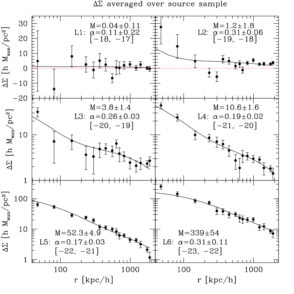
Figure 1: Weak lensing signal $\Delta\Sigma(r)$ as a function of transverse separation $r$ as measured from SDSS data, together with the best fit 2-parameter model for each of 6 luminosity bins. Also shown are the best fit values for halo virial mass $M$ (in units of $10^{11}h^{-1}M_{\hbox{$\odot$}}$) and $\alpha$, the fraction of galaxies that are non-central, assuming $M_{\rm nl}=8\times 10^{12}M_{\hbox{$\odot$}}$. The model fits the data well in all bins. The mass fits are what comes from the fitting procedure and are a typical halo mass somewhere between mean and median. For bias calculations they are increased by varying amounts to account for the difference between fitted mass and mean mass, as described in the text.

We repeat the analysis by adding more parameters to the fit. The most relevant parameter for bias is $\epsilon$, which changes the relative proportion of less massive versus more massive halos for the non-central component. We find that we cannot determine all 3 parameters separately at each luminosity bin, so that $\epsilon$ is strongly anti-correlated with $\alpha$. For example, we find that even solutions with $\epsilon=2$ are allowed, suggesting a large fraction of massive halos. However, at the same time $\alpha$ is reduced, so that the overall fraction of massive halos is more or less unchanged. This is exactly what one would expect, since the signal at $R=300-2000h^{-1}$kpc is measuring directly the contribution from these massive halos (groups and clusters). In other words, the 3-parameter fit is essentially a non-parametric fit to the data with large degeneracies between the parameters, but little variation in the halo mass probability distribution in the relevant range.

We also tried a different nonparametric fit, where we divide the halo masses into several bins and fit for the fraction in each separately. Not surprisingly we find huge degeneracies between individual components in this case, especially at the low mass end. Even in this most general case the fraction of galaxies residing in large halos (above $10^{14}h^{-1}M_{\hbox{$\odot$}}$) is constrained to be below 0.2 at the bright end and below 0.01 at the faint end. It is particularly important that the fraction of galaxies in these high mass halos is strongly constrained, as these halos have the largest bias and a poor constraint on them leads to a larger error on the bias predictions. The variations of bias consistent with these various halo mass probability distributions are in fact very small.

While for standard analysis we assumed that radial distribution of galaxies is the same as that of dark matter, we also explored other possibilities. Weak lensing data have some sensitivity to determine the radial distribution directly, since a shallow galaxy distribution also leads to a shallow radial dependence of $\Delta\Sigma$ Mandelbaum et al. (2004). However, this only makes a difference at large radii and the central mass determination only weakly depends on it. We find that the central halo mass changes by less than 10% if $c_{g}$ is varied by a factor of 2 from its assumed value $c_{\rm dm}$.

One possible source of systematical error is the shear calibration from measured ellipticities. For this analysis using re-Gaussianization, as shown in Mandelbaum et al. (2005), when we include all sources of shear calibration error (not just the 2-3% PSF dilution correction), we are left with a roughtly 10% shear calibration error ($2\sigma$).

The redshifts of background galaxies are another possible source of systematic error. For those galaxies that have photometric redshifts the main difficulty is knowing the error distribution, since even a relatively minor fraction of outliers can skew the distribution and lead to a bias in the lensing signal. This is particularly problematic for the brighter galaxies ($r<21$) for which the typical redshift is 0.2-0.4. We use direct matching of SDSS objects with deeper spectroscopic surveys (DEEP2) to calibrate our photometric redshifts. An independent analysis using Luminous Red Galaxies (LRG) for which we know the redshift error distribution, provides an independent confirmation of our photoz calibration. Details of the LRG redshift distributions are given in Padmanabhan et al. (2004), and the comparison with the other methods used for this paper is in Mandelbaum et al. (2005).

The redshift distributions as a function of magnitude are relatively well measured at these magnitudes, so one could use those instead of photometric redshifts. However, the existing redshift distributions that apply to the overall population of galaxies cannot be directly used in the lensing analysis, especially not at the faint end. This is because a significant fraction of galaxies are rejected or downweighted in the lensing analysis because they are too small to give reliable ellipticity measurements. These galaxies tend to be smaller and thus at a higher redshift relative to the overall population. So the effective redshift of the “lensing weighted” population tends to be lower than that of the overall population at the same magnitude. The same effect may also lead to an underestimate of $\sigma_{8}$ in weak lensing measurements of the power spectrum, where it can have much more damaging consequences. It is very difficult to account for this effect if one does not have the complete redshift information of a representative portion of the data.

Besides the shear calibration and redshift distribution, there are several other sources of systematic error in the weak lensing signal: magnification bias, stellar contamination, intrinsic alignments, sky level determination errors. We use estimates of the values of these errors for our analysis from Mandelbaum et al. (2005), and place a 10% $1-\sigma$ overall calibration error on the lensing signal on top of the (comparable) statistical errors.

III.3 Bias predictions

In the next step we take the results from the previous section to compute the predicted bias as a function of luminosity. Bias is a nonlinear function of the model parameters and we wish to determine both the mean and the variance. The fits for the halo mass probability distribution can be strongly degenerate, so a Gaussian approximation for the fitted parameters is not necessarily valid. In addition, one must impose physical constraints such as $\alpha>0$ and $M_{0}>0$. Our approach is to use bootstrap resampling to determine the errors. We divide the observed area into 200 chunks of roughly equal area. We then bootstrap resample these, by randomly choosing 200 chunks with replacement (so some of these are duplicated). We perform the fitting procedure as described above on each of the bootstrap realizations. We use the fitted parameters to compute the bias using equation 12. Finally, we compute the mean and variance of the bias parameter by averaging over 2500 of these bootstrap resamplings.

Before discussing the results we need to address the redshift evolution. Redshift evolution can affect the weak lensing analysis, the bias analysis and the clustering analysis. Most of the galaxies are at low redshift up to $z\sim 0.2$ (table 1), so any corrections due to the redshift evolution are small. Moreover, there are various competing effects that further suppress the redshift evolution effects.

We work in comoving coordinates, so redshift effects are minor. One usually applies the evolution correction to the galaxy luminosity to account for the fact that higher redshift galaxies are brighter because their stars are younger. We use the correction as given in Blanton et al. (2003c), adding the quantity $1.6(z-0.1)$ to the $r$-band absolute magnitudes. This correction is not important as long as we use the same definition of luminosity in our weak lensing analysis as is in the clustering analysis. The definition of the virial mass as defined by FOF algorithm of simulations is in comoving coordinates: FOF algorithm finds clusters with a density contrast of order $b^{-3}$ relative to the mean, where $b$ is the linking length of FOF. This definition does not vary with redshift in comoving coordinates. The main effect of redshift evolution is that nonlinear mass at higher redshifts is lower, which affects the mass function and bias predictions. We perform the analysis on a grid of nonlinear masses defined at z=0 and for each use the nonlinear mass value appropriate for the median redshift for a given luminosity bin. Regarding the clustering evolution with redshift, for $L_{*}$ galaxies a typical redshift is 0.1, so once we find bias for these galaxies and multiply it with the observed amplitude of galaxy clustering we need to evolve this amplitude of fluctuations to redshift 0, which increases it by roughly 5% in a $\Lambda$CDM universe.

The results for 2-parameter models are shown in figure 2 for several values of the nonlinear mass $M_{\rm nl}$, spanning the range from $1.6\times 10^{11}h^{-1}M_{\hbox{$\odot$}}$ (corresponding to $\sigma_{8}=0.6$, $\Omega_{m}=0.2$ model) at the top to $2.5\times 10^{13}h^{-1}M_{\hbox{$\odot$}}$ (corresponding to $\sigma_{8}=1.1$, $\Omega_{m}=0.3$ model) at the bottom (we vary $\sigma_{8}$ from 1.1 to 0.6 from bottom up assuming $\Omega_{m}=0.3$, the top one has $\sigma_{8}=0.6$ and $\Omega_{m}=0.25$). Note that the weak lensing determination of $\alpha$ depends on $M_{\rm nl}$, since the cluster contribution depends on the cluster mass function: for higher value of nonlinear mass the exponential cutoff in the mass function is at a higher mass and so the fraction of galaxies in this component can be lower to match the observational constraints. We include this by performing the lensing analysis on all the values of $M_{\rm nl}$ of interest and use that information when computing bias predictions as a function of $M_{\rm nl}$.

One can see that as a consequence of the weak lensing determination of the halo mass distribution models with low nonlinear masses (low $\sigma_{8}$ and/or $\Omega_{m}$) predict higher bias than those with higher nonlinear masses. Notice how the models with high nonlinear mass predict almost constant bias with luminosity, a consequence of bias being independent of mass below 0.1$M_{\rm nl}$. On the other hand, if nonlinear mass is close to the halo mass of $L_{*}$ galaxies then the bias is rapidly changing with luminosity.

We can address the robustness of the bias predictions by comparing the results between 2 and 3-parameter models. These are shown in table 1 for nonlinear mass $M_{\rm nl}=5.6\times 10^{12}h^{-1}M_{\hbox{$\odot$}}$, corresponding to the $\sigma_{8}=0.9$, $\Omega_{m}=0.27$ model. 3-parameter models are very degenerate and often give unlikely values such as $\epsilon=0$ (corresponding to the case where the number of galaxies within a halo is constant regardless of halo mass). This is compensated by increasing the value of $\alpha$ so that the data are still fit well. Remarkably, the mean bias and its error hardly change from 2-parameter models to 3-parameter models in all bins. This demonstrates that the bias predictions are robust against the parametrization of the halo probability distribution.

Figure 2: This figure shows the lensing-constrained model predictions for bias as a function of nonlinear mass using the 2-parameter models of the halo mass probability distribution. More general models of the halo probability distribution give very similar results and are not shown here. The nonlinear masses from top to bottom are $3.4\times 10^{11}h^{-1}M_{\hbox{$\odot$}}$, $6.2\times 10^{11}h^{-1}M_{\hbox{$\odot$}}$, $1.7\times 10^{12}h^{-1}M_{\hbox{$\odot$}}$, $4.0\times 10^{12}h^{-1}M_{\hbox{$\odot$}}$, $8.0\times 10^{12}h^{-1}M_{\hbox{$\odot$}}$, $1.5\times 10^{13}h^{-1}M_{\hbox{$\odot$}}$ and $2.4\times 10^{13}h^{-1}M_{\hbox{$\odot$}}$. Errors have been suppressed (see Table 1).

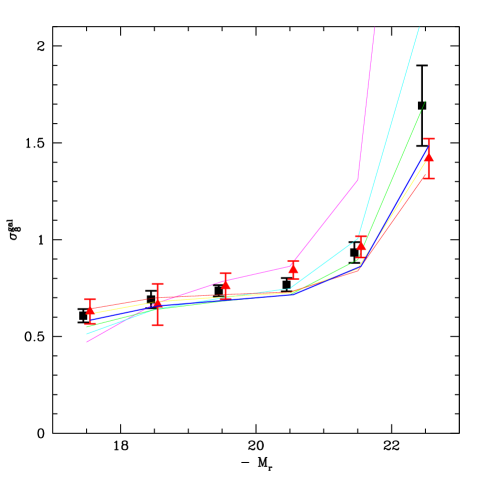
Figure 3: The halo bias predictions of galaxy fluctuation amplitude $\sigma_{8}^{\rm gal}$ as a function of luminosity varying linear matter amplitude $\sigma_{8}$: 0.6, 0.7, 0.8, 0.9, 1.0, 1.1, from top to bottom on the right hand side. The remaining parameters have been fixed to $\Omega_{m}=0.3$ and $n_{s}=1$. Squares are for model with $\sigma_{8}=0.88$, $n_{s}=1.0$ and $\Omega_{m}=0.3$. For this model we show errors from theoretical modelling. Also shown as triangles are the observed values of $\sigma_{8}^{\rm gal}$.

Figure 3 shows the predicted values for galaxy clustering amplitude $\sigma_{8}$ for models with $\sigma_{8}$ varying from 0.6 to 1.1, with $\sigma_{8}=0.88$ in bold. This is obtained by taking predicted bias values and multiply them with $\sigma_{8}$. Also shown is the observed values of $\sigma_{8}$ which are obtained by taking $b/b_{*}$ values in table 1 and multiplying them with $\sigma_{8}(M_{{{}^{0.1}\!{r}}}=-20.8)=0.875$ value as obtained from Tegmark et al. (2003b). The latter is almost independent on cosmological parameters and has a statistical error of 0.013. The first thing to notice is the agreement between the theoretical predictions and the observations, with theoretical predictions being slightly lower than observations at L4. Theoretical models predict both the gradual flattening of bias for galaxies fainter than L4, as well as a rapid increase in bias from L5 to L6, both of which are observed in SDSS data. This rapid increase in bias from L5 to L6 is caused both by the rapid increase in bias above the nonlinear mass as well as by the rapid decrease in star formation efficiency for the most massive halos: going from L5 to L6 we increase the luminosity by a factor of 2.5, while the halo mass has increased by a factor of 6.5 (figure 1), and the fraction of non-central galaxies has also increased. So the scaling between halo mass and luminosity becomes much steeper at the bright end and most of the galaxies in the $[-22,-23]$ bin reside in group and cluster halos with masses above $10^{13}h^{-1}M_{\hbox{$\odot$}}$.

This agreement between the theoretical bias predictions and observations suggests that a fundamental prediction of large scale structure models, that of the bias dependence on halo mass, has been confirmed. Very low values of $M_{\rm nl}$ predict that bias is rapidly changing with mass over the observed range, which is not observed. On the other side of the mass range, very high values of $M_{\rm nl}$ predict bias is changing very slowly with mass, which would also be in contradiction with the observations. These results constrain $\sigma_{8}$, but these constraints by themselves are not very strong. In fact, one can find good agreement for $\sigma_{8}\sim 0.7-1.0$.

At first this agreement between theoretical predictions and observations is so good it is almost disappointing, since the two agree over a broad range of $M_{\rm nl}$. While this result confirms the basic prediction of the structure formation models it would appear that it does not allow us to place useful constraints on cosmological models. This conclusion is too pessimistic, since nonlinear mass is also changed by varying $\Omega_{m}$ and slope $n_{s}$. For example, reducing $\Omega_{m}$ to 0.27 from 0.3 and $n_{s}$ to 0.96 from 1 reduces nonlinear mass by a factor of 2 and increases theoretical bias predictions by 10% at L4. This brings the observations into a better agreement with theoretical predictions and improves the fit to $\chi^{2}\sim 7$ at $\sigma_{8}=0.88$. The data thus favor slightly lower values of $\Omega_{m}$ or $n_{s}$ than their canonical values of 0.3 and 1, respectively. We note that this analysis is strongly sensitive on the accuracy of the bias as a function halo mass relation and we would find very different conclusions using expressions in Jing (1998); Sheth and Tormen (1999) over the more recent ones in Seljak and Warren (2004).

These heuristic arguments are formalized in the next section, where we incorporate the bias constraints into the parameter estimation procedure. It is clear from this discussion that the bias constraints depend on nonlinear mass, which in turn depends on several cosmological parameters such as $\sigma_{8}$, $\Omega_{m}$ and $n_{s}$, so the best strategy is to perform a full analysis over the parameter space of interest.

However, it is worth highlighting where the strongest constraints are coming from and explore if the bias determination of flux limited sample would improve the cosmological constraints. One can see from figure 2 that for $L4$ in the range $\sigma_{8}=0.6-0.9$ all models give essentially the same value of $\sigma_{8}(L4)\sim 0.75$, which is lower than the observed value of 0.85. Similarly, we can take the predictions for bias as a function of luminosity and weight it by galaxy numbers (given in table 1) to obtain the bias prediction for the flux limited sample. This has the advantage that it can be related to the observed value which has very small errors, $\sigma_{8}(M_{{{}^{0.1}\!{r}}}=-20.8)=0.88\pm 0.02$. However, the predictions are almost independent of $\sigma_{8}$: we find 0.77 at $\sigma_{8}=0.7$ and 0.73 at $\sigma_{8}=1$ for $\Omega_{m}=0.3$ and $n_{s}=1$. The fact that the predictions are lower than observed value again argues that these two parameters (or shape parameter $\Gamma$ which depends on Hubble parameter $h$ as well) must be lower. Therefore, using the flux limited sample amplitude one cannot determine the bias and $\sigma_{8}$ despite a relatively small error on the observationally determined amplitude of galaxy clustering. The reason for that is the degeneracy in the way bias changes with amplitude of fluctuations: reducing $\sigma_{8}$ by 10% reduces $M_{\rm nl}$ by a factor of 2 and increases bias predictions around $M=M_{\rm nl}$ by 10%, so the product $b\sigma_{8}$, which determines the galaxy clustering amplitude, remains unchanged. We find that by using the full range of luminosity breaks this degeneracy, because the bias is very slowly changing with nonlinear mass on one end and very strongly changing with it on the other end of luminosity range.

III.4 Bias error budget

We will include the following $\chi^{2}$ component in the overall likelihood evaluation,

$$\chi^{2}=\sum_{i=1}^{6}{\left(b_{\rm model,i}-b_{*}(b/b_{*})_{\rm i}\right)^{2}\over\sigma_{b_{\rm model,i}}^{2}+b_{*}^{2}\sigma_{b/b_{*},i}^{2}+\sigma_{\rm sys}^{2}},$$ (13)

where $b_{\rm model,i}$ is the predicted bias for the i-th luminosity bin and $\sigma_{b_{\rm model,i}}$ the corresponding error, $(b/b_{*})_{\rm i}$ is the observed bias at the same luminosity and $\sigma_{b/b_{*},i}$ the corresponding error and $\sigma_{\rm sys}=0.03$ accounts for systematic uncertainties in the theoretical modeling of the bias and its variations with the model Seljak and Warren (2004). For a given model we first compute $M_{\rm nl}$ and then interpolate between the values shown in figure 2 to obtain $b_{\rm model,i}$ and $\sigma_{b_{\rm model,i}}$. Note that $b_{*}$ is one of the parameters we are varying and is constrained both by the $\chi^{2}$ above and by the overall amplitude of the galaxy power spectrum. For $b_{\rm model,i}$ we use the 2-parameter fits as given in table 1, although using the 3-parameter fits would give almost identical results.

Equation 13 contains 3 contributions to the bias error. First is the error on the theoretical bias prediction, $\sigma_{b_{\rm model,i}}$. This error is dominated by the uncertainties in the conditional halo mass probability distribution $p(M;L)$. Despite significant uncertainties in the probability distributions (specially for the 18 parameter fits) the resulting values of $\sigma_{b_{\rm model,i}}$ are between 0.02-0.08 for $M_{\rm nl}\sim 10^{13}h^{-1}M_{\hbox{$\odot$}}$. This is typically smaller than the errors on the observed bias $\sigma_{b/b_{*},i}$, which range from 0.054 to 0.12. We assign a systematic uncertainty $\sigma_{\rm sys}=0.03$ to all of the bins except the brightest one (L6), where we use $\sigma_{\rm sys}=0.1$ to account for larger variations in model predictions, as well as larger systematic uncertainties due to the rapid variation of the bias with luminosity and redshift. The systematic error is subdominant compared to the clustering or lensing error. Current bias constraints are mostly dominated by the observational uncertainties in the bias from the clustering analysis and not by the modeling uncertainties of either the bias or conditional halo mass probability distribution as determined by weak lensing. Note that systematic uncertanties in calibration and redshift distribution have already been included in the lensing analysis and corresponds to about 0.03 in bias. The current statistical error in the bias, averaging over all 6 bins in table 1, is 0.03, so the systematic error is at most equal to the statistical error.

Much of the error budget in $\sigma_{b/b_{*},i}$ is due to the sampling variance. We are treating the bias estimates as uncorrelated between luminosity bins, assuming they come from independent volumes. In reality there is some overlap in volume between neighboring luminosity bins and some of the same large scale structure contributes to two bins at the same time (see e.g. figure 3 in Tegmark et al. (2003b)). Because of this our error estimation is conservative, since for overlapping regions sampling variance between luminosity subsamples should be reduced. The reduction is however rather modest even for very large scales Seljak and Warren (2004). Note that systematic uncertainties lead to some correlations between the errors, which we ignore in the present analysis since they are small. It would be straightforward to generalize upon this by computing the correlations between the bootstrap samples.

IV Cosmological parameter determination

In this section we include the bias constraints in the parameter determination procedure to see if we can constrain cosmological models better than without this information. We combine the constraints from the SDSS power spectrum with CMB observations from WMAP (Bennett et al., 2003; Hinshaw et al., 2003; Kogut et al., 2003). We implement the Monte Carlo Markov Chain method (Christensen and Meyer, 2001) using CMBFAST version 4.5 Seljak and Zaldarriaga (1996), outputting both the CMB spectra and the corresponding matter power spectra $P(k)$. We evolve all the matter power spectra to a high $k$ using CMBFAST and we do not employ any analytical approximations. In addition, we use linear to nonlinear mapping of the matter power spectrum using expressions given in Smith et al. (2003).

Our implementation of the MCMC is the same as in Seljak et al. (2003). It is independent of that used in Tegmark et al. (2003a), but we verified that the results for the case of WMAP+SDSS without bias agree. A typical run is based on 48 independent chains, contains 50,000-200,000 chain elements and requires 2-4 days of running on a 48 processor cluster in a serial mode of CMBFAST. The success rate was of order 30-50%, correlation length (as defined in Tegmark et al. (2003a)) 10-30 and the effective chain length of order 3,000-20,000. We use 23-39 chains and in terms of Gelman and Rubin $\hat{R}$-statistics (Gelman and Rubin, 1992) we find the chains are sufficiently converged and mixed, with $\hat{R}<1.05$, ie we are more conservative than the recommended value $\hat{R}<1.2$.

Our pivot point is at $k=0.05/$Mpc and we use the tensor normalization convention in which for the simplest inflationary models the tensor to scalar ratio is $r=T/S=-8n_{T}$. Our most general parameter space is

$$\hbox{\boldmath{$p$}}=(\tau,\omega_{b},\omega_{m},m_{\nu},\Omega_{\lambda},{\cal R},n_{s},\alpha_{s},T/S,b_{*}),$$ (14)

where $\tau$ is the optical depth, $\omega_{b}=\Omega_{b}h^{2}$ is proportional to the baryon to photon density ratio, $\omega_{m}=\Omega_{m}h^{2}$ is proportional to the matter to photon density ratio, $m_{\nu}$ is the massive neutrino mass, $\Omega_{\lambda}$ is the dark energy density today and $w$ its equation of state, ${\cal R}$ is the amplitude of curvature perturbations at $k=0.05$/Mpc, $n_{s}$ is the scalar slope at the same pivot and $\alpha_{s}=dn_{s}/d\ln k$ is the running of the slope, which we approximate as constant. We fix the tensor slope $n_{T}$ using $T/S=-8n_{T}$. We do not allow for non-flat models, since curvature is already tightly constrained by CMB and other constraints, which leads to $\Omega_{K}=0.02\pm 0.02$ for the simplest models Spergel et al. (2003). For the more general models, such as those with dark energy equation of state, relaxing this assumption can lead to a significant expansion of errors. We are therefore testing a particular class of models with $K=0$ and not presenting model independent constraints on equation of state. We follow the WMAP team in imposing a $\tau<0.3$ constraint. Upcoming polarization data from WMAP will allow a verification of this prior. From this basic set of parameters we can obtain constraints on several other parameters, such as the baryon and matter densities $\Omega_{b}$ and $\Omega_{m}$, Hubble parameter $h$ and amplitude of fluctuations $\sigma_{8}$. Since we do now allow for curvature one has $\Omega_{\lambda}=1-\Omega_{m}$ and we use $\Omega_{m}$ in table 2. In fact, our primary parameter is $\Theta_{s}$, the angular scale of the acoustic horizon, which is tightly constrained by the CMB. Similarly, although we use ${\cal R}$ as the primary parameter in the MCMC we present the amplitude in terms of the more familiar $\sigma_{8}$.

The basic result for two different MCMC runs are given in table 2 for SDSS combined with WMAP. For most of the parameters we quote the median value (50%), [15.84%,84.16%] interval ($\pm 1\sigma$), and [2.3%,97.7%] interval ($\pm 2\sigma$). These are calculated from the cumulative one-point distributions of MCMC values for each parameter and do not depend on the Gaussian assumption. For the parameters without a detection we only quote a 95% confidence limit. All of the restricted parameter space fits are acceptable based on $\chi^{2}$ values, starting from the 6-parameter model with no tensors, running or neutrino mass. Introducing additional parameters does not improve the fit significantly. However, we wish to determine the amplitude of fluctuations in an as model independent way as possible and for this reason we explore the most general parameter space possible.

Below we discuss the results from this table in more detail. Our standard model has 6 cosmological parameters: $\tau,\omega_{b},\omega_{m},\Omega_{\lambda}=1-\Omega_{m},{\cal R},n_{s}$, plus “nuisance parameter” bias $b_{*}$. For the case without bias our results are in a broad agreement with those in Tegmark et al. (2003a), although a slightly different treatment (modification of lowest multipoles in WMAP and inclusion of $\tau<0.3$ constraint) does lead to small changes in the best fit parameters and their errors.

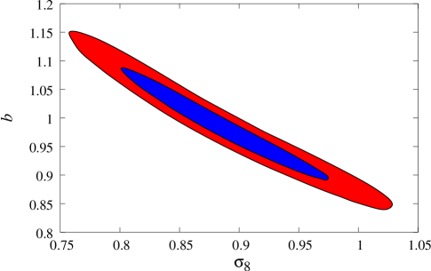
Figure 4: 68% (inner, blue) and 95% (outer, red) contours in $(\sigma_{8},b_{*})$ plane using SDSS+WMAP+bias measurements. The two parameters are strongly correlated because only their product is determined from SDSS clustering analysis. The additional bias constraint helps reduce the degeneracy.

IV.1 $\sigma_{8}$ and bias

Table 2: median value, $1\sigma$ and $2\sigma$ constraints on cosmological parameters combining CMB, SDSS power spectrum shape and SDSS bias information. The columns compare different theoretical priors. The parameters for 7 parameter models are $\tau,\omega_{b},\omega_{m},\Omega_{\lambda}=1-\Omega_{m},{\cal R},n_{s}$, plus “nuisance parameter” bias $b_{*}$.

	7par	7par+T/S	7par+$m_{\nu}$	7par+$\alpha_{s}$	7par+T/S+$m_{\nu}$+$\alpha_{s}$
$10^{3}\omega_{b}$	$23.4^{+1.2}_{-1.1}{}^{+2.5}_{-2.1}$	$25.1^{+1.6}_{-1.5}{}^{+3.4}_{-2.8}$	$23.7^{+1.3}_{-1.2}{}^{+2.5}_{-2.2}$	$22.9^{+1.4}_{-1.4}{}^{+2.8}_{-2.7}$	$24.8^{+1.6}_{-1.6}{}^{+3.3}_{-3.1}$
$\Omega_{m}$	$0.253^{+0.027}_{-0.026}{}^{+0.053}_{-0.047}$	$0.226^{+0.027}_{-0.026}{}^{+0.055}_{-0.053}$	$0.259^{+0.031}_{-0.027}{}^{+0.074}_{-0.048}$	$0.269^{+0.041}_{-0.033}{}^{+0.091}_{-0.062}$	$0.262^{+0.051}_{-0.036}{}^{+0.138}_{-0.072}$
$n_{s}$	$0.987^{+0.037}_{-0.031}{}^{+0.071}_{-0.055}$	$1.040^{+0.045}_{-0.042}{}^{+0.094}_{-0.078}$	$0.995^{+0.037}_{-0.034}{}^{+0.065}_{-0.060}$	$0.959^{+0.052}_{-0.053}{}^{+0.104}_{-0.106}$	$1.00^{+0.054}_{-0.058}{}^{+0.118}_{-0.121}$
$\tau$	$0.181^{+0.068}_{-0.066}{}^{+0.110}_{-0.116}$	$0.187^{+0.063}_{-0.062}{}^{+0.103}_{-0.119}$	$0.202^{+0.064}_{-0.072}{}^{+0.092}_{-0.130}$	$0.195^{+0.065}_{-0.068}{}^{+0.097}_{-0.123}$	$0.232^{+0.046}_{-0.064}{}^{+0.064}_{-0.127}$
$b_{*}$	$0.984^{+0.070}_{-0.065}{}^{+0.129}_{-0.119}$	$0.965^{+0.068}_{-0.062}{}^{+0.131}_{-0.113}$	$1.02^{+0.079}_{-0.074}{}^{+0.157}_{-0.137}$	$0.970^{+0.069}_{-0.060}{}^{+0.133}_{-0.106}$	$0.986^{+0.078}_{-0.065}{}^{+0.158}_{-0.115}$
$\sigma_{8}$	$0.884^{+0.064}_{-0.057}{}^{+0.120}_{-0.098}$	$0.904^{+0.062}_{-0.60}{}^{+0.121}_{-0.105}$	$0.854^{+0.066}_{-0.060}{}^{+0.127}_{-0.112}$	$0.896^{+0.058}_{-0.058}{}^{+0.108}_{-0.104}$	$0.882^{+0.062}_{-0.063}{}^{+0.116}_{-0.119}$
$h$	$0.732^{+0.034}_{-0.031}{}^{+0.065}_{-0.056}$	$0.773^{+0.042}_{-0.038}{}^{+0.097}_{-0.071}$	$0.728^{+0.034}_{-0.034}{}^{+0.067}_{-0.069}$	$0.716^{+0.039}_{-0.039}{}^{+0.078}_{-0.079}$	$0.738^{+0.045}_{-0.050}{}^{+0.100}_{-0.112}$
$T/S$	0	$<0.49$ (95%)	0	0	$<0.57$ (95%)
$m_{\nu}$	0	0	$<0.18$eV (95%)	0	$<0.24$eV (95%)
$\alpha_{s}$	0	0	0	$-0.024^{+0.031}_{-0.031}{}^{+0.062}_{-0.061}$	$-0.045^{+0.036}_{-0.040}{}^{+0.073}_{-0.089}$

Figure 4 shows the 68% and 95% contours in the $(\sigma_{8},b_{*})$ plane. The two parameters are strongly correlated because the SDSS power spectrum constrains their product to be $b_{*}\sigma_{8}=0.87\pm 0.02$. Both bias and $\sigma_{8}$ are in a good agreement with the SDSS+WMAP analysis without bias constraints, which gives for the basic 6-parameter model $b_{*}=0.96\pm 0.08$ and $\sigma_{8}=0.92\pm 0.09$ Tegmark et al. (2003a), but which in the presence of massive neutrinos changes to $b_{*}=1.06\pm 0.10$ and $\sigma_{8}=0.82\pm 0.09$. We find $\sigma_{8}=0.88\pm 0.06$ and $b_{*}=0.99\pm 0.07$ in the presence of neutrinos and running with bias constraints included. There remains a significant degeneracy between $\sigma_{8}$ and optical depth $\tau$, as shown in figure 5. The upcoming WMAP polarization analysis may help improve this degeneracy.

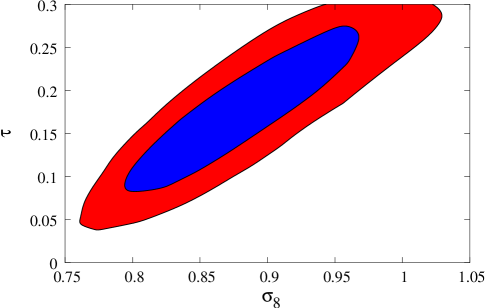
Figure 5: 68% (inner, blue) and 95% (outer, red) contours in $(\sigma_{8},\tau)$ plane using SDSS+WMAP+bias measurements. There is a correlation between the two, so a better determination of optical depth $\tau$ from polarization data would help improve the constraints.

Let us now compare these constraints to other methods to determine bias and $\sigma_{8}$. The closest analysis to ours is that of the WMAP+2dF bispectrum using $k\sim(0.2-0.3)h$/Mpc modes. Our $\sigma_{8}$ is in a good agreement with the WMAP+2dF analysis with the bias constraint from the bispectrum, which gives $\sigma_{8}=0.84\pm 0.04$. The 2dF bispectrum analysis has been performed on scales smaller than the scale of the power spectrum analysis ($k<0.2h/$Mpc), so many of subsequent analysis papers chose not to adopt this constraint. The fact that a completely independent approach presented here finds the same result is therefore encouraging and suggests that the systematics are not dominating the statistical errors in either approach.

There are several other methods of $\sigma_{8}$ determination, such as cluster abundance, weak lensing and Sunyaev-Zeldovich effect. Cluster abundance estimations of $\sigma_{8}$ range from 0.6 to 1, often with very small errors (see a recent overview of the current situation in Tegmark et al. (2003a)). Many of these are reported for $\Omega_{m}=0.3$, so if the actual value is somewhat lower the required value for $\sigma_{8}$ increases. The main difficulty is in calibrating the mass-temperature relation, which cannot be done with simulations, because these still lack some of the physics of cluster formation such as cooling, feedback, conduction etc. Direct calibration from the mass and temperature measurements on individual clusters is more promising, but is limited by statistical and systematic errors. With this method the results are particularly sensitive to calibration errors at various steps of the analysis, so the challenge for the future will be to control them at the required level.

Weak lensing observations also have a similar spread in reported values of $\sigma_{8}$ (between 0.7 and 1, see overview in Tegmark et al. (2003a)). The assigned statistical errors are larger, so there may not be much conflict among different observations. In addition, with this method there are also systematic calibration effects at the 10-20% level in $\sigma_{8}$. Some of these are discussed in in the context of present analysis in §III.B, but a similar discussion applies to other weak lensing analyses as well. These are often not included in the error budget. As discussed above, these arise both for shear calibration from ellipticity measurements and for the redshift distribution of background galaxies.

Finally, CBI Mason et al. (2003); Readhead et al. (2004) and BIMA Dawson et al. (2002) measurements of the CMB at high $l$ find excess power, which can be interpreted as a Sunyaev-Zeldovich signal. If so this would require a fairly high normalization, with estimates of $\sigma_{8}$ ranging from $0.98^{+0.06}_{-0.07}$ Readhead et al. (2004) to $1.04\pm 0.12({\rm stat})\pm 0.1({\rm sys})$ (Komatsu and Seljak, 2002), where both errors are 2-sigma. Some of the difference between the two estimates is due to the drop of the CBI amplitude in the latest analysis, while the rest is due to the differences in the modeling of the signal from either simulations or analytic models.

In summary, our value of $\sigma_{8}$ is consistent with most recently reported values. It is at the lower end of what is required to explain the CBI/BIMA excess power in terms of the SZ effect and at the upper end of some of the weak lensing and cluster abundance measurements. Each one of these may have additional systematic errors that could bring the results into a better agreement. Our values are in excellent agreement with the WMAP+2dF analysis.

IV.2 Neutrino mass

Galaxy surveys are important as tracers of neutrino mass, since neutrinos have a considerable effect on the matter power spectrum. At the time of decoupling such neutrinos are still relativistic, but become nonrelativistic later in the evolution of the universe if their mass is sufficiently high. Neutrinos free-stream out of their potential wells, erasing their own perturbations on scales smaller than the so-called free streaming length, defined as the distance at which a neutrino of a given rms velocity $v_{\rm th}$ can still escape against gravity. The velocity is $c$ when neutrinos are relativistic and drops as $1/a$ afterwords because of momentum conservation, so

$$v_{\rm th}\sim{k_{B}T\over m_{\nu}}=50(1+z)(m_{\nu}/{\rm eV})^{-1}{\rm km/s}.$$ (15)

Since the comoving Hubble time is proportional to $\tau_{H}\sim[(1+z)\Omega_{m}]^{-1/2}H_{0}^{-1}$ the product of the two gives an estimate of the free-streaming length. The resulting comoving free-streaming wavevector is (for one massive family)

$$k_{fs}=0.4(\Omega_{m}h^{2})^{1/2}(1+z)^{-1/2}{m_{\nu}\over 1{\rm eV}}{\rm Mpc}^{-1}.$$ (16)

It should be evaluated at redshift when neutrinos become non-relativistic, since the dominant contribution comes from when neutrinos are relativistic.

For a given wavevector $k$ neutrino perturbations are suppressed while $k>k_{fs}$. After that they can grow again and may even catch up with the matter perturbations. When neutrinos are dynamically important the neutrino damping also affects the matter fluctuations, decreasing their amplitude on scales below the free streaming length. One can see from equation 16 that the scale is fairly large for the neutrino masses of interest, $k_{\rm fs}\sim 0.1{\rm Mpc}^{-1}$ at $z=0$ for $m_{\nu}\sim 1eV$. Below this suppression scale the power spectrum shape is the same as in regular CDM models, so on small scales the only consequence is the suppression of the amplitude (see figure 6). We can thus adopt the halo bias predictions from CDM models and apply them to massive neutrino models as well. We should note that while qualitatively the effects are similar for 1 or 3 massive neutrino families, they differ in detail (figure 6), so the constraints are not directly comparable and one must do a separate analysis in the two cases. We mostly focus on 3 degenerate neutrino families here, but also present MCMC results for 3 massless+1 massive family below.

While it is commonly believed that massive neutrinos have a minor effect on the CMB, this is actually not entirely the case for the masses of interest below 2eV. This is because neutrinos with such a low mass are still relativistic when they enter the horizon for scales around $k=0.1h$/Mpc and are either relativistic or quasi-relativistic at the time of recombination, $z\sim 1100$ (equation 15). As a result neutrinos cannot be treated as a nonrelativistic component with regard to the CMB. Figure 6 shows how much the CMB spectrum changes for various neutrino masses relative to the zero mass case, keeping $\Omega_{m}=\Omega_{\rm cdm}+\Omega_{b}+\Omega_{\nu}$ constant (as well as the other cosmological parameters). One can see that for $m_{\nu}=0.3$eV massive neutrinos increase the spectrum by 6% at $l=200$, well above the errors (neutrinos are also not degenerate with respect to the CMB if we compare them to a fixed $\Omega_{\rm cdm}+\Omega_{b}$ instead). In addition, massive neutrinos increase the CMB spectrum but suppress the power spectrum (figure 6), which enhances the sensitivity when the two tracers are combined.

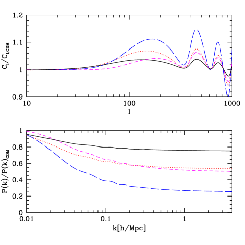
Figure 6: Top panel shows the change in CMB spectrum $C_{l}$ for several neutrino masses relative to zero mass. The masses are $m_{\nu}=0.15$eV (solid, black), 0.3eV (dotted, red) and 0.6eV (long dashed, blue), all with 3 neutrino families of equal mass. Also shown (short dashed) is the case of 3 massless + 1 massive neutrino family with $m_{\nu}=0.9$eV. Bottom shows the ratio of matter power spectra for the same models. We see that while increasing neutrino mass increases the CMB spectrum it decreases the matter power spectrum. For the same total mass the 3+1 model is more non-relativistic at recombination, has a smaller effect on the CMB spectrum relative to 3 families of equal mass and the corresponding mass limits are weaker.

We note that our bias constraints significantly improve upon neutrino mass limits. In the absence of biasing constraints the neutrino mass limit from WMAP+SDSS is $m_{\nu}<0.6$eV if their masses are nearly degenerate Tegmark et al. (2003a). Biasing constraints improve significantly upon this. We find

$$m_{\nu}<0.18{\rm eV}(95\%)~{}{\rm(3~{}families,~{}without~{}running)},$$ (17)

at 95% for a single component if we assume no running, as was done in all of the work to date. Our constraints improve upon WMAP+2dF constraints, where $m_{\nu}<0.23$eV was found by combining WMAP and 2dF with the bias determination from the bispectrum analysis (Verde et al., 2002).

However, this result was based on the assumption of no running. This assumption was present in all of the work so far, including Spergel et al. (2003) where it was argued that there is a weak evidence of running. A running spectral index changes the shape of the power spectrum as the massive neutrinos do, so including the running in the parameter estimation can significantly expand the limits. Naive expectations are that a negative running (which seems to be preferred by the data) suppresses the power on small scales just as a massive neutrino and so would lead to a tighter constraint on neutrino mass, but MCMC analysis does not confirm this and the constraints are weakened. With biasing constraints and running our constraint changes to

$$m_{\nu}<0.24{\rm eV}(95\%)~{}{\rm(3~{}families,~{}with~{}running)}.$$ (18)

All of the mass limits presented here are based on 3 degenerate massive neutrino families. If one assumes a model with 3 massless families and 1 massive family (a sterile neutrino model), as motivated by LSND Athanassopoulos et al. (1996), then the mass limits on the sum change, since both the CMB and and the transfer function change. One finds the limits are significantly weakened: in the WMAP+2dF analysis without bias the limit is 1.4eV Hannestad (2003). We find the same

$$m_{\nu}<1.37{\rm eV}(95\%)~{}{\rm(3+1~{}families,~{}no~{}running)}.$$ (19)

The reason for the relatively weak constraint is that this case is much more degenerate with $\Omega_{m}$ than the case of 3 degenerate massive neutrino families. From the LSND experiment the allowed regions are four islands with the lowest mass $m_{\nu}=0.9$eV and the next lowest 1.4eV Maltoni et al. (2003). We see that the windows are rapidly closing with cosmological constraints, but the case is not yet air tight.

There were recent claims that the neutrino mass may have already been detected from cosmological observations (Allen et al., 2003a). These claimed detections are inconsistent with our WMAP+SDSS or with WMAP+2dF constraints and are based primarily on the cluster abundance analysis of Allen et al. (2003b), which seems to prefer a low value for the amplitude, $\sigma_{8}\sim 0.7$. As discussed above, cluster abundance estimates of $\sigma_{8}$ range from 0.6 to 1 and are likely to be dominated by systematics often not included in the quoted errors, such as mass-temperature calibration. Increasing the error on this method to account for systematics removes the evidence for neutrino mass.

V Discussion and Conclusions

In this paper we presented a detailed comparison between observations and theoretical predictions of one of the fundamental predictions of structure formation models, that of linear bias as a function of halo mass. In doing so we combine two separate observational analyses of SDSS data, the galaxy clustering analysis and a weak lensing analysis, both as a function of galaxy luminosity. The former gives us the relative bias as a function of luminosity, while the latter connects the galaxies of a given luminosity class to their dark matter halo mass distribution. We find a remarkable agreement between the observations and theoretical predictions of bias over a range of halo masses from $10^{11}h^{-1}M_{\hbox{$\odot$}}$ to $10^{13}h^{-1}M_{\hbox{$\odot$}}$. This success should be viewed as an important new confirmation of the current large scale structure paradigm in predicting the properties of the universe we live in.

The second goal of this work is to provide a determination of the bias for SDSS galaxies, which can be used to improve the cosmological parameter estimation. For any given model we can determine bias from the halo mass-bias relation and from the amplitude of galaxy clustering. The two must agree, which requires the bias of $M_{{{}^{0.1}\!{r}}}=-20.8$ galaxies to be very close to unity. As a result we can place constraints on the amplitude of fluctuations, $\sigma_{8}=0.88\pm 0.06$, as well as on the other other cosmological parameters. Our results are in an excellent agreement with the WMAP+2dFGRS analysis of Spergel et al. (2003). In particular, we find no evidence for any systematic differences between the SDSS and 2dF power spectra in either amplitude or shape.

The systematic errors from the galaxy clustering data have been thoroughly examined in Tegmark et al. (2003b), but some open question remain to be addressed. One of them is the correction for nonlinear effects in the power spectrum analysis. These can affect both the conversion from redshift space to real space and from the real space power spectrum to the linear power spectrum. The current analysis in Tegmark et al. (2003b) is based on the power spectrum with $k<0.2h$/Mpc, but this cutoff is somewhat arbitrary and should be justified within a more realistic model, which will provide an estimate of the systematic error as a function of $k$. Currently the nonlinear corrections are based on the nonlinear evolution model of Smith et al. (2003). However, galaxies are not a perfect tracer of dark matter and the nonlinear correction for galaxies could be different from that of dark matter. For example, in the context of halo models nonlinear effects are entirely due to the correlations within the halos. If galaxies populate larger (smaller) halos than the dark matter then the nonlinear corrections will be larger (smaller). The halo model is not sufficiently accurate to address these questions in detail and simulations are needed instead. To put things in perspective, the overall galaxy clustering amplitude $b_{*}\sigma_{8}$ from SDSS using $k<0.2h$/Mpc data points has an error of 1.5%, while the nonlinear correction at $k=0.2h$/Mpc is around 10%. In this situation it does not take much for the systematic error to dominate over the statistical error. However, much of the error will be on the overall amplitude and this is still limited by the error on our bias determination, which is around 7%. Nonlinear effects are likely to be even more important for the luminosity dependent analysis of galaxy clustering, which was used in this paper as a basis for bias determination, but statistical errors in this analysis are larger and systematics may not dominate the results. It is clear that these issues have to be revisited if one is to believe the cosmological implications from these results.

We have argued that the method presented here is in many ways more robust than some of the other methods to determine the bias from observations. Still, there remain possible systematic errors in the present analysis that need to be explored further. Two uncertainties mentioned in the present analysis are the calibration of the weak lensing signal and the accuracy of the bias-halo mass relation. We have argued that the weak lensing method is robust in that even a 20% calibration error leads to only 0.03 error in bias. This does not dominate relative to the statistical error and we have included it in the analysis. Similarly, the bias-halo mass relation has been calibrated to an accuracy of 0.03 using a suite of large simulations covering some of the parameter space of interest Seljak and Warren (2004), but larger simulations and more extensive grid of parameter space is needed to improve this to an accuracy of 0.01.

The current paper should be viewed as a first application of this method of bias determination, rather than the last word on it. There are many ways the current analysis could be improved. The most important among these is reducing the error on the clustering amplitude as a function of luminosity, specially for low luminosity galaxies. As we argued most of the leverage for bias determination comes from the low luminosity galaxies, which reside in low mass halos, and for which the bias is only weakly dependent on the nonlinear mass (it is also relatively insensitive to errors in the lensing analysis). A better analysis optimized to reduce the sampling variance errors should reduce the errors considerably. Galaxies with absolute luminosities in the range $[-18,-20]$ seem particularly promising, since they have a reliable lensing detection (figure 1) and a weak bias dependence on nonlinear mass (figure 2), unless the nonlinear mass is very low. Their clustering amplitude is currently very poorly determined compared to the overall sample (Table 1), which could be improved dramatically with a more careful analysis. In addition, the systematic errors in the lensing analysis could be reduced further. All of these aspects can be improved in the near future. This could lead to significant improvements on the cosmological parameters such as neutrino mass or equation of state.

The present paper is only the first in several possible attempts to estimate the large scale bias in SDSS. An ongoing project closest to our approach is to use the galaxy auto-correlation function on small scales to constrain the halo occupation probability distribution. A bispectrum analysis of SDSS galaxies is also in progress and should yield results which are statistically comparable to the present analysis. A weak lensing analysis on large scales can also determine the bias, although this would require larger survey areas than currently available and a tight control of all possible systematics. Current efforts are limited to small scales and their statistical power remains weak Sheldon et al. (2003). Finally, with better modeling of redshift space distortions the constraints on $\beta$ may also improve beyond the current limits, which at the moment remain weak Tegmark et al. (2003b). Combining and comparing these with the current analysis will provide additional checks of systematics in these methods.

The method presented here can be applied to other samples of galaxies, such as those selected by color, spectral type or stellar mass. Of particular interest would be to apply it to the higher redshift galaxies, such as the Luminous Red Galaxies, which are very numerous in surveys such as SDSS and whose photometric redshifts are relatively accurate and well understood. Their clustering amplitude on large scales can be determined with a high accuracy, close to 1%, in several redshift bins up to $z=0.7$. Without a model for bias the amplitude does not give useful information. If one could determine their halo mass distribution function with lensing that would allow one to predict the bias and thus extract the growth factor as a function of redshift. While the absolute calibrations of bias are still difficult at a 1% level, the relative calibration as a function of redshift may be more promising. This may be one of the most promising methods to place constraints on the dark energy equation of state and its evolution.

Funding for the creation and distribution of the SDSS Archive has been provided by the Alfred P. Sloan Foundation, the Participating Institutions, the National Aeronautics and Space Administration, the National Science Foundation, the U.S. Department of Energy, the Japanese Monbukagakusho, and the Max Planck Society. The SDSS Web site is http://www.sdss.org/. We thank M. Strauss, P. Steinhardt and L. Verde for useful comments.

The SDSS is managed by the Astrophysical Research Consortium (ARC) for the Participating Institutions. The Participating Institutions are The University of Chicago, Fermilab, the Institute for Advanced Study, the Japan Participation Group, The Johns Hopkins University, Los Alamos National Laboratory, the Max-Planck-Institute for Astronomy (MPIA), the Max-Planck-Institute for Astrophysics (MPA), New Mexico State University, University of Pittsburgh, Princeton University, the United States Naval Observatory, and the University of Washington.

Our MCMC simulations were run on a Beowulf cluster at Princeton University, supported in part by NSF grant AST-0216105. US is supported by fellowships from the David and Lucile Packard Foundation, Alfred P. Sloan Foundation, NASA grants NAG5-1993, NAG5-11489 and NSF grant CAREER-0132953. MT was supported by NSF grant AST-0134999, NASA grant NAG5-11099 and fellowships from the David and Lucile Packard Foundation and the Cottrell Foundation.

Funding for the DEEP2 survey has been provided by NSF grant AST-0071048 and AST-0071198. Some of the data presented herein were obtained at the W.M. Keck Observatory, which is operated as a scientific partnership among the California Institute of Technology, the University of California and the National Aeronautics and Space Administration. The Observatory was made possible by the generous financial support of the W.M. Keck Foundation. The DEEP2 team and Keck Observatory acknowledge the very significant cultural role and reverence that the summit of Mauna Kea has always had within the indigenous Hawaiian community and appreciate the opportunity to conduct observations from this mountain.

References

- Hatton and Cole (1998) S. Hatton and S. Cole, MNRAS 296, 10 (1998).
- Scoccimarro et al. (2001) R. Scoccimarro, R. K. Sheth, L. Hui, and B. Jain, ApJ 546, 20 (2001).
- Seljak (2001) U. Seljak, MNRAS 325, 1359 (2001).
- Percival et al. (2002) W. J. Percival, W. Sutherland, J. A. Peacock, C. M. Baugh, J. Bland-Hawthorn, T. Bridges, R. Cannon, S. Cole, M. Colless, C. Collins, et al., MNRAS 337, 1068 (2002).
- Tegmark et al. (2003a) M. Tegmark, M. Strauss, M. Blanton, K. Abazajian, S. Dodelson, H. Sandvik, X. Wang, D. Weinberg, I. Zehavi, N. Bahcall, et al., ArXiv eprint astro-ph/0310723 (2003a).
- Davis and Geller (1976) M. Davis and M. J. Geller, ApJ 208, 13 (1976).
- Norberg et al. (2001) P. Norberg, C. M. Baugh, E. Hawkins, S. Maddox, J. A. Peacock, S. Cole, C. S. Frenk, J. Bland-Hawthorn, T. Bridges, R. Cannon, et al., MNRAS 328, 64 (2001).
- Zehavi et al. (2002) I. Zehavi, M. R. Blanton, J. A. Frieman, D. H. Weinberg, H. J. Mo, M. A. Strauss, S. F. Anderson, J. Annis, N. A. Bahcall, M. Bernardi, et al., ApJ 571, 172 (2002).
- Tegmark et al. (2003b) M. Tegmark, M. Blanton, M. Strauss, F. Hoyle, D. Schlegel, R. Scoccimarro, M. Vogeley, D. Weinberg, I. Zehavi, A. Berlind, et al., ArXiv e-print astro-ph/0310725 (2003b).
- Verde et al. (2002) L. Verde, A. F. Heavens, W. J. Percival, S. Matarrese, C. M. Baugh, J. Bland-Hawthorn, T. Bridges, R. Cannon, S. Cole, M. Colless, et al., MNRAS 335, 432 (2002).
- Hoekstra et al. (2002) H. Hoekstra, L. van Waerbeke, M. D. Gladders, Y. Mellier, and H. K. C. Yee, ApJ 577, 604 (2002).
- Sheldon et al. (2003) E. S. Sheldon, D. E. Johnston, J. A. Frieman, R. Scranton, T. A. McKay, A. J. Connolly, T. Budavari, I. Zehavi, N. Bahcall, J. Brinkmann, et al. (2003).
- Hirata et al. (2004) C. M. Hirata, R. Mandelbaum, U. Seljak, J. Guzik, N. Padmanabhan, C. Blake, J. Brinkmann, T. Budavari, A. Connolly, I. Csabai, et al. (2004), eprint astro-ph/0403255.
- Cole and Kaiser (1989) S. Cole and N. Kaiser, MNRAS 237, 1127 (1989).
- Mo and White (1996) H. J. Mo and S. D. M. White, MNRAS 282, 347 (1996).
- Sheth and Tormen (1999) R. K. Sheth and G. Tormen, MNRAS 308, 119 (1999).
- Sheth et al. (2001) R. K. Sheth, H. J. Mo, and G. Tormen, MNRAS 323, 1 (2001).
- Jing (1998) Y. P. Jing, ApJ 503, L9+ (1998).
- Seljak and Warren (2004) U. Seljak and M. S. Warren, ArXiv e-print astro-ph/0403698 (2004), eprint astro-ph/0403698.
- Guzik and Seljak (2002) J. Guzik and U. . Seljak, MNRAS 335, 311 (2002).
- Tyson et al. (1984) J. A. Tyson, F. Valdes, J. F. Jarvis, and A. P. Mills, ApJ 281, L59 (1984).
- Brainerd et al. (1996) T. G. Brainerd, R. D. Blandford, and I. Smail, ApJ 466, 623 (1996).
- Hudson et al. (1998) M. J. Hudson, S. D. J. Gwyn, H. Dahle, and N. Kaiser, ApJ 503, 531+ (1998).
- Fischer et al. (2000) P. Fischer, T. A. McKay, E. Sheldon, A. Connolly, A. Stebbins, J. A. Frieman, B. Jain, M. Joffre, D. Johnston, G. Bernstein, et al., AJ 120, 1198 (2000).
- Smith et al. (2001) D. R. Smith, G. M. Bernstein, P. Fischer, and M. Jarvis, ApJ 551, 643 (2001).
- McKay et al. (2001) T. A. McKay, E. S. Sheldon, J. Racusin, P. Fischer, U. Seljak, A. Stebbins, D. Johnston, J. A. Frieman, N. Bahcall, J. Brinkmann, et al. (2001), eprint astro-ph/0108013.
- Sheldon et al. (2004) E. S. Sheldon, D. E. Johnston, J. A. Frieman, R. Scranton, T. A. McKay, A. J. Connolly, T. Budavári, I. Zehavi, N. A. Bahcall, J. Brinkmann, et al., AJ 127, 2544 (2004).
- Hirata and Seljak (2003) C. Hirata and U. Seljak, MNRAS 343, 459 (2003).
- Mandelbaum et al. (2005) R. Mandelbaum, C. Hirata, U. Seljak, J. Guzik, N. Padmanabhan, C. Blake, M. R. Blanton, R. Lupton, and J. Brinkmann, ArXiv Astrophysics e-prints (2005), eprint astro-ph/0501201.
- Yang et al. (2003) X. Yang, H. J. Mo, and F. C. van den Bosch, MNRAS 339, 1057 (2003).
- van den Bosch et al. (2003) F. C. van den Bosch, H. J. Mo, and X. Yang, MNRAS 345, 923 (2003).
- Press and Schechter (1974) W. H. Press and P. Schechter, ApJ 187, 425 (1974).
- Jenkins et al. (2001) A. Jenkins, C. S. Frenk, S. D. M. White, J. M. Colberg, S. Cole, A. E. Evrard, H. M. P. Couchman, and N. Yoshida, MNRAS 321, 372 (2001).
- White (2001) M. White, A&A 367, 27 (2001).
- Seljak (2002) U. Seljak, MNRAS 337, 774 (2002).
- Navarro et al. (1996) J. F. Navarro, C. S. Frenk, and S. D. M. White, ApJ 462, 563+ (1996).
- Bullock et al. (2001) J. S. Bullock, T. S. Kolatt, Y. Sigad, R. S. Somerville, A. V. Kravtsov, A. A. Klypin, J. R. Primack, and A. Dekel, MNRAS 321, 559 (2001).
- Eke et al. (2001) V. R. Eke, J. F. Navarro, and M. Steinmetz, ApJ 554, 114 (2001).
- Kauffmann et al. (1999) G. Kauffmann, J. M. Colberg, A. Diaferio, and S. D. M. White, MNRAS 303, 188 (1999).
- Kravtsov et al. (2003) A. V. Kravtsov, A. A. Berlind, R. H. Wechsler, A. A. Klypin, S. Gottloeber, B. Allgood, and J. R. Primack (2003).
- Mandelbaum et al. (2004) R. Mandelbaum, A. Tasitsiomi, U. Seljak, A. V. Kravtsov, and R. H. Wechsler, ArXiv Astrophysics e-prints (2004), eprint astro-ph/0410711.
- Tasitsiomi et al. (2004) A. Tasitsiomi, A. V. Kravtsov, R. H. Wechsler, and J. R. Primack, ArXiv Astrophysics e-prints (2004), eprint astro-ph/0404168.
- York et al. (2000) D. G. York, J. Adelman, J. E. Anderson, S. F. Anderson, J. Annis, N. A. Bahcall, J. A. Bakken, R. Barkhouser, S. Bastian, E. Berman, et al., AJ 120, 1579 (2000).
- Gunn et al. (1998) J. E. Gunn, M. Carr, C. Rockosi, M. Sekiguchi, K. Berry, B. Elms, E. de Haas, Ž. Ivezić, G. Knapp, R. Lupton, et al., AJ 116, 3040 (1998).
- Fukugita et al. (1996) M. Fukugita, T. Ichikawa, J. E. Gunn, M. Doi, K. Shimasaku, and D. P. Schneider, AJ 111, 1748 (1996).
- Stoughton et al. (2002) C. Stoughton, R. H. Lupton, M. Bernardi, M. R. Blanton, S. Burles, F. J. Castander, A. J. Connolly, D. J. Eisenstein, J. A. Frieman, G. S. Hennessy, et al., AJ 123, 485 (2002).
- Pier et al. (2003) J. R. Pier, J. A. Munn, R. B. Hindsley, G. S. Hennessy, S. M. Kent, R. H. Lupton, and Ž. Ivezić, AJ 125, 1559 (2003).
- Hogg et al. (2001) D. W. Hogg, D. P. Finkbeiner, D. J. Schlegel, and J. E. Gunn, AJ 122, 2129 (2001).
- Smith et al. (2002) J. A. Smith, D. L. Tucker, S. Kent, M. W. Richmond, M. Fukugita, T. Ichikawa, S. Ichikawa, A. M. Jorgensen, A. Uomoto, J. E. Gunn, et al., AJ 123, 2121 (2002).
- Abazajian et al. (2004) K. Abazajian, J. K. Adelman-McCarthy, M. A. Agüeros, S. S. Allam, K. S. J. Anderson, S. F. Anderson, J. Annis, N. A. Bahcall, I. K. Baldry, S. Bastian, et al. (2004), eprint astro-ph/0403325.
- Strauss et al. (2002) M. A. Strauss, D. H. Weinberg, R. H. Lupton, V. K. Narayanan, J. Annis, M. Bernardi, M. Blanton, S. Burles, A. J. Connolly, J. Dalcanton, et al., AJ 124, 1810 (2002).
- Blanton et al. (2003a) M. R. Blanton, H. Lin, R. H. Lupton, F. M. Maley, N. Young, I. Zehavi, and J. Loveday, AJ 125, 2276 (2003a).
- Blanton et al. (2003b) M. R. Blanton, J. Brinkmann, I. Csabai, M. Doi, D. Eisenstein, M. Fukugita, J. E. Gunn, D. W. Hogg, and D. J. Schlegel, AJ 125, 2348 (2003b).
- Padmanabhan et al. (2004) N. Padmanabhan, T. Budavari, D. J. Schlegel, T. Bridges, J. Brinkmann, R. Cannon, A. J. Connolly, S. M. Croom, I. Csabai, M. Drinkwater, et al. (2004), eprint astro-ph/0407594.
- Blanton et al. (2003c) M. R. Blanton, D. W. Hogg, N. A. Bahcall, J. Brinkmann, M. Britton, A. J. Connolly, I. Csabai, M. Fukugita, J. Loveday, A. Meiksin, et al., ApJ 592, 819 (2003c).
- Bennett et al. (2003) C. L. Bennett, M. Halpern, G. Hinshaw, N. Jarosik, A. Kogut, M. Limon, S. S. Meyer, L. Page, D. N. Spergel, G. S. Tucker, et al., ApJS 148, 1 (2003).
- Hinshaw et al. (2003) G. Hinshaw, D. N. Spergel, L. Verde, R. S. Hill, S. S. Meyer, C. Barnes, C. L. Bennett, M. Halpern, N. Jarosik, A. Kogut, et al., ApJS 148, 135 (2003).
- Kogut et al. (2003) A. Kogut, D. N. Spergel, C. Barnes, C. L. Bennett, M. Halpern, G. Hinshaw, N. Jarosik, M. Limon, S. S. Meyer, L. Page, et al., ApJS 148, 161 (2003).
- Christensen and Meyer (2001) N. Christensen and R. Meyer, Phys. Rev. D 64, 22001 (2001).
- Seljak and Zaldarriaga (1996) U. Seljak and M. Zaldarriaga, ApJ 469, 437 (1996).
- Smith et al. (2003) R. E. Smith, J. A. Peacock, A. Jenkins, S. D. M. White, C. S. Frenk, F. R. Pearce, P. A. Thomas, G. Efstathiou, and H. M. P. Couchman, MNRAS 341, 1311 (2003).
- Seljak et al. (2003) U. Seljak, P. McDonald, and A. Makarov, MNRAS 342, L79 (2003).
- Gelman and Rubin (1992) A. Gelman and D. Rubin (1992).
- Spergel et al. (2003) D. N. Spergel, L. Verde, H. V. Peiris, E. Komatsu, M. R. Nolta, C. L. Bennett, M. Halpern, G. Hinshaw, N. Jarosik, A. Kogut, et al., ApJS 148, 175 (2003).
- Mason et al. (2003) B. S. Mason, T. J. Pearson, A. C. S. Readhead, M. C. Shepherd, J. Sievers, P. S. Udomprasert, J. K. Cartwright, A. J. Farmer, S. Padin, S. T. Myers, et al., ApJ 591, 540 (2003).
- Readhead et al. (2004) A. C. S. Readhead, B. S. Mason, C. R. Contaldi, T. J. Pearson, J. R. Bond, S. T. Myers, S. Padin, J. L. Sievers, J. K. Cartwright, M. C. Shepherd, et al., ArXiv e-print astro-ph/0402359 (2004), eprint astro-ph/0402359.
- Dawson et al. (2002) K. S. Dawson, W. L. Holzapfel, J. E. Carlstrom, M. Joy, S. J. LaRoque, A. D. Miller, and D. Nagai, ApJ 581, 86 (2002).
- Komatsu and Seljak (2002) E. Komatsu and U. Seljak, MNRAS 336, 1256 (2002).
- Athanassopoulos et al. (1996) C. Athanassopoulos, L. B. Auerbach, R. L. Burman, I. Cohen, D. O. Caldwell, B. D. Dieterle, J. B. Donahue, A. M. Eisner, A. Fazely, F. J. Federspiel, et al., Physical Review Letters 77, 3082 (1996).
- Hannestad (2003) S. Hannestad, Journal of Cosmology and Astro-Particle Physics 5, 4 (2003).
- Maltoni et al. (2003) M. Maltoni, T. Schwetz, M. A. Tórtola, and J. W. F. Valle, Nuclear Physics B Proceedings Supplements 114, 203 (2003).
- Allen et al. (2003a) S. W. Allen, R. W. Schmidt, and S. L. Bridle (2003a).
- Allen et al. (2003b) S. W. Allen, R. W. Schmidt, A. C. Fabian, and H. Ebeling, MNRAS 342, 287 (2003b).