A decreasing column density during the prompt emission from GRB000528 observed with BeppoSAX

Abstract

We report observation results of the prompt X– and $\gamma$–ray emission from GRB 000528. This event was detected with the Gamma-Ray Burst Monitor and one of the two Wide Field Cameras aboard the BeppoSAX satellite. The GRB was promptly followed on with the BeppoSAX Narrow Field Instruments and with ground optical and radio telescopes. The X–ray afterglow source was identified, but no optical or radio counterpart found. We report here results from the prompt and afterglow emission analysis. The main feature derived from spectral evolution of the prompt emission is a high hydrogen-equivalent column density with evidence of its decrease with time. We model this behavior in terms of a time-dependent photoionization of the local circum-burst medium, finding that a compact and dense environment is required by the data. We also find a fading of the late part of the 2–10 keV prompt emission which is consistent with afterglow emission. We discuss this result in the light of the external shock model scenario.

1 Introduction

The prompt emission of long duration ($>$2 s) Gamma Ray Bursts (GRBs) in the broad 2–700 keV energy band, which was accessible to the BeppoSAX wide field instruments (Wide Field Cameras, Jager et al. 1997 , and Gamma Ray Burst Monitor, Frontera et al. 1997), has been demonstrated to provide information not only on the X–ray emission mechanisms of GRBs but also on their environments (e.g., Frontera et al. 2000, Frontera 2004a). The properties of these environments are of key importance to unveil the nature of the GRB progenitors, which is a still open issue. Many observational results point to the collapse of massive stars, in particular to the explosion of type Ic supernovae, as the most likely progenitors of long GRBs. However the simultaneity of the GRB event and supernova explosion (hypernova model, e.g., Paczynski 1998), in spite of the convincing results obtained from GRB0303289 Stanek et al. (2003); Hijorth et al. (2003), cannot be considered a solved problem for all GRBs. A two-step process, in which first the massive star gives rise to a supernova explosion with the formation of a neutron star, and thus, after some time, to a GRB from the delayed collapse of the NS to a BH (supranova model, Vietri & Stella 1998) or from a phase transition to quark matter Berezhiani et al. (2003) cannot be robustly excluded. At least in some cases (e.g., GRB990705, Amati et al. 2000 ; GRB011211, Frontera et al. 2004b, GRB991216, Piro et al. 2000), in which X–ray transient absorption features or emission lines have been observed and found consistent with an Iron-enriched environment typical of a previous supernova explosion, the two–step process is favored (Lazzati et al. 2001a, 2001b, 2002).

The properties of the GRB environment can also be derived from the study of the continuum spectrum of the prompt X–ray emission, which is expected to show a low-energy cutoff in case of a high column density along the line of sight. If the absorbing material is located between a fraction of a parsec to several parsecs from the GRB site, the cutoff is expected to fade as the GRB evolves. This is due to the progressive photoionization of the gas by the GRB photons (e.g., Böttcher et al. 1999; Lazzati & Perna 2002). This is an effect analogous to the one originally proposed by Perna & Loeb (1998) in the optical domain with resonant lines. Actually, such cutoffs, with also evidence of their decreasing behaviour with time from the GRB onset, have already been detected (GRB980506, Connors & Hueter 1998; GRB980329, Frontera et al. 2000). Lazzati & Perna (2002) interpreted them as evidence for presence of overdense regions in molecular clouds with properties similar to those of star formation globules.

Now we report the discovery of another case of absorption. It has been found in the X–ray spectrum of the prompt emission of GRB000528, in the context of a systematic investigation Frontera et al. 2004c performed to study the spectral evolution of all GRBs jointly detected with WFCs and GRBM. GRB000528, detected with the GRBM Guidorzi et al. (2000) and localised with the BeppoSAX WFC Gandolfi (2000), was promptly followed-up with the BeppoSAX Narrow Field Instruments (NFI), with the discovery in the WFC error box of a likely X–ray afterglow candidate of the burst Kuulkers et al. (2000). However neither an optical or radio counterpart was found (lowest upper limit to the $R$ magnitude of 23.3, Palazzi et al. 2000; 3.5$\sigma$ upper limit of 0.14 mJy at 8.46 GHz, Berger & Frail 2000).

In this paper we report our findings and their interpretation. We also discuss the follow–up X–ray observations performed with the BeppoSAX NFIs and their implications.

2 BeppoSAX observations

GRB000528 was detected with the BeppoSAX WFC No. 2 and GRBM Gandolfi (2000) on 2000 May 28 at 08:46:21 UT. The GRB position was determined with an error radius of $2^{\prime}$ (99% confidence level) and was centered at $\alpha_{2000}=10^{\rm h}45^{\rm m}06.3^{\rm s}$, and $\delta_{2000}=-33^{\circ}58^{\prime}59^{\prime\prime}$ in ’t Zand et al. (2000). The burst was then followed–up with the NFIs two times, the first time (TOO1) from May 28.71 UT to May 29.57 UT (from 8.25 to 28.90 hrs after the main event), and the second time (TOO2) from May 31.65 UT to June 1.49 UT (from 3.284 to 4.124 days from the main event). Two previously unknown sources, the first one (S1) designated 1SAX J1045.5$-$3358, with coordinates $\alpha_{2000}=10^{\rm h}45^{\rm m}28^{\rm s}$, and $\delta_{2000}=-33^{\circ}58^{\prime}14^{\prime\prime}$, the second one (S2) designated 1SAX J1045.1$-$3358, with coordinates $\alpha_{2000}=10^{\rm h}45^{\rm m}08^{\rm s}$, and $\delta_{2000}=-33^{\circ}59^{\prime}26^{\prime\prime}$ were detected with MECS and both found to have disappeared in TOO2 Kuulkers et al. (2000). However only the S2 position (uncertainty radius of 1.5^′) was found consistent with the WFC error box (see also Hurley et al. 2000).

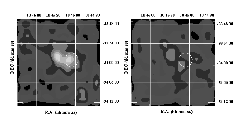
Figure 1: 2–10 keV image of the sky field obtained with MECS in the two BeppoSAX follow–up observations of GRB000528. The first TOO started 8.25 hrs after the burst, the second 3.284 days later. The error box obtained with the WFC 2 is also shown.

We have reanalysed the MECS and LECS data. The exposure times of the two instruments to the GRB direction are 8084 s (LECS) and 26589 s (MECS) in TOO1, and 6905 s (LECS) and 31210 s (MECS) in TOO2. The images of the sky field derived with MECS 2+3 during the two TOOs are shown in Fig. 1, with superposed the WFC error box. The two sources reported by Kuulkers et al. are clearly visible in the left image. The probability that the excesses found are due to background fluctuations is $\sim 7\times 10^{-7}$. The source S1, which is out of the WFC error box, is coincident with a radio source, which was already present in the NRAO VLA Sky Survey (NVSS) at the time of the GRB occurrence. It was again detected by Berger & Frail (2000) during the search of the radio counterpart of GRB000528. This source is also detected in the second observation (chance probability of $\sim 5\times 10^{-4}$), with a flux variation by a factor 1.7 from the first to the second TOO. However the source S2 is detected only during the first TOO, it is consistent with the WFC position, and undergows a flux decrease larger than a factor 3 from the first to the second TOO (see Section 3.2). As already concluded by Kuulkers et al. (2000), we assume this object as the likely afterglow source of GRB000528.

3 Data analysis and results

The spectral analysis of both the prompt and afterglow emission was performed with the xspec software package Arnaud (1996), version 11.2. All the reported parameter uncertainties are given at 90% confidence level.

3.1 Prompt emission

Data available from GRBM include 1 s ratemeters in the two energy channels (40–700 keV and $>$100 keV), 128 s count spectra (40–700 keV, 225 channels) and high time resolution data (up to 0.5 ms) in the 40–700 keV energy band. WFCs were operated in normal mode with 31 channels in 2–28 keV and 0.5 ms time resolution. The burst direction was offset by 8.0^∘ with respect to the WFC axis. With this offset, the effective area exposed to the GRB was $\approx$ 340 cm² in the 40-700 keV band and 70 cm² in the 2–28 keV energy band. The background in the GRBM energy band was estimated by linear interpolation using the 250 s count rate data before and after the burst. The WFC spectra were extracted through the Iterative Removal Of Sources procedure (IROS , e.g. Jager et al. 1997 ) which implicitly subtracts the contribution of the background and of other point sources in the field of view.

Figure 2 shows the light curve of GRB000528 in two energy bands. In X–rays (top panel of Fig. 2) it shows a seemingly long rise with superposed various small pulses until it achieves the highest peak at a level of 300 cts s^-1 after $\sim 70$ s from the onset. Then the X–ray flux starts to smoothly decay and ends after $\sim 120$ s from the flux peak. In gamma–rays the light curve (bottom panel of Fig. 2) is totally different. In correspondence of the first of the secondary pulses of the X–ray light curve we find the most prominent gamma-ray pulse, where the GRB achieves the maximum count rate in the 40–700 keV band of 1700 counts s^-1. Instead, in correspondence of the peak flux in X–rays we only find a secondary pulse of the gamma–ray light curve. Smaller and shorter duration pulses are also visible in the gamma–ray light curve. However the smooth decay of the X–ray light curve is not observed in gamma–rays and the entire duration of the 40–700 keV burst is only $\sim 80$ s versus the $\sim 160$ s duration in X–rays.

For the study of the GRB spectral shape and its evolution with time, we extracted the WFC and GRBM data in the same time intervals and we simultaneously fitted the WFC and GRBM data. For GRBM we used both types of data available: the 1 s counters and the 128 s spectra. Using the counters we had the possibility to subdivide the GRB light curve in 6 adjacent time intervals A, B, C, D, E, F of 18, 11, 10, 20, 20 and 90 s duration, respectively (see Fig. 2) and to derive 2–700 keV count spectrum for each of these intervals. The obtained GRB count spectra are shown in Fig. 3. Given that the first three spectra (A, B, and C) have a low statistical quality in the 2-28 keV band, for the fitting analysis they were summed together (interval ABC). Using 128 s GRBM transmitted spectra, we obtained two 2–700 keV spectra in the two time intervals 1 and 2, whose boundary time is marked in Fig. 2. The interval 1 covers the ABC interval above, while the interval 2 covers the intervals D, E and F.

Each of the four spectra (ABC, D, E, F) was fit with various continuum models: a power-law (pl), a power-law with an exponential cutoff (cpl), a broken power-law (bknpl), a smoothly broken power-law (or Band law, bl, Band et al. 1993). All these models were assumed to be photoelectrically absorbed by an equivalent–hydrogen column density $N_{\rm H}$ to be determined (the wabs model in xspec). In the fits, the normalisation factor of the GRBM data with respect to WFC was left free to vary, checking that its best fit value was in the range (0.8 to 1.3) in which this parameter was found in the flight calibrations with either celestial sources (e.g., Crab Nebula) or GRBs observed with both the WFC-GRBM and the BATSE experiment aboard the Compton Gamma Ray Observatory (e.g., Fishman et al. 1994). The power–law model gave a completely unacceptable fit of all count spectra either assuming the Galactic column density along the GRB line of sight ($N_{\rm H}^{\rm G}=6.1\times 10^{20}$ cm^-2) or leaving the $N_{\rm H}$ free to vary in the fit. The fit with the Band law gave in general unconstrained parameters. The other two models (cpl), and bknpl) resulted the most suitable to describe the data. The fit results with these models are reported in Table 1, along with the $\chi^{2}/dof$ value either in the case $N_{\rm H}$ is frozen to the Galactic value ($N_{\rm H}^{\rm G}$) or in the case it is left free to vary in the fit.

Apart from the typical hard-to-soft evolution of the spectrum with time, the most remarkable feature found is the value of the column density $N_{\rm H}$, which results to be higher than the Galactic value in the first three time intervals ABC, D and E (see chance probabilities obtained with F-test in Table 1) and it is consistent with 0, and thus with $N_{\rm H}^{\rm G}$, in the interval F (2$\sigma$ upper limit reported in Table 1). As can be seen from the F test values, these results are independent of the spectral model chosen (bknpl or cpl). We notice that, altough with lower significance, these results are confirmed with fits using WFC data only. Also the analysis of the two GRBM 128 s spectra are consistent with these results. Both spectra were well fit with either a bknpl or cpl. In both cases a column density $N_{\rm H}=N_{\rm H}^{\rm G}$ does not give the best description of the data (see Table 1); a best fit is obtained with $N_{\rm H}$ values significantly higher than the Galactic column density.

Even if we cannot completely exclude a constantly high $N_{\rm H}$, the data are in favour of a decreasing column density. Indeed, summing together the data in the intervals ABC and D, we estimate an $N_{\rm H}=1.0_{-0.3}^{+0.4}\times 10^{23}$ cm^-2, which is not consistent with the highest 2$\sigma$ upper limit of the $N_{\rm H}$ in the interval F ($4.4\times 10^{22}$ cm^-2) and it is only marginally consistent with its $3\sigma$ upper limit. In addition, we find that the $N_{\rm H}$ centroid is continuously decreasing with time (see Fig. 4) and the fit of the $N_{\rm H}$ values with a constant (weighted mean value $5.8\pm 1.1\times 10^{23}$ cm^-2) gives a $\chi^{2}/dof$ value of 7.8/3, versus a value of 0.65/2 in the case of an exponential law ($N_{\rm H}(t)=N_{0}\exp(-t/t_{0})$). Using the F-test Bevington (1969), the probability that a constant $N_{\rm H}$ value is the real parent distribution is 6%. Finally the comparison of the light curves in the 2–10 keV and 10–28 keV energy bands (Fig. 4) are also suggestive of a variable $N_{\rm H}$. Assuming the above exponential law, the best fit parameters of the exponential law are $N_{0}=(2.4\pm 1.2)\times 10^{23}$ cm^-2 and $t_{0}=51\pm 23$ s.

No evidence of an absorption edge associated with the variable $N_{\rm H}$ is found in the spectra. The upper limit to the edge optical depth $\tau$ depends on the energy assumed and on the time interval considered. With the continuum parameters fixed to their best fit values obtained with the cpl, the $2\sigma$ $\tau$ upper limit achieves the lowest value (0.2) at 5 keV in interval D and the highest value (1.8) at 2 keV in the interval ABC. The other upper limits are in between.

On the basis of the best fit results, peak fluxes and fluences associated with the event were derived. The 2–10 keV and 40–700 keV peak fluxes in 1 s time bin are $F_{2-10}=2.1\times 10^{-8}$  erg cm^-2 s^-1and $F_{40-700}=1.4\times 10^{-6}$  erg cm^-2 s^-1, while the fluences are given by $S_{2-10}=9.1\times 10^{-7}$ erg cm^-2, and $S_{40-700}=1.37\times 10^{-5}$ erg cm^-2, with a softness ratio $SR=S_{2-10}/S_{40-700}=0.066$, which is a value typical of a classic GRB (e.g., Frontera et al. 2000). Finally the total 2–700 keV fluence of the GRB is given by $S_{2-700}=1.9\times 10^{-5}$ erg cm^-2.

3.2 Afterglow emission

Due to the weakness of the afterglow source (see Fig. 1), no statistically significant spectral information could be derived. Assuming the average power-law photon index (1.95) derived from the spectra of a large sample of GRB afterglows Frontera 2003a , from the MECS data we estimated the afterglow source flux in the two observations of GRB000528, using an image extraction radius of 2^′ and adopting the MECS standard background level. The resulting 2–10 keV mean flux is $(1.6\pm 0.4)\times 10^{-13}$  erg cm^-2 s^-1($1\sigma$ uncertainty) during TOO1 and less than $5.2\times 10^{-14}$  erg cm^-2 s^-1($2\sigma$ upper limit) for TOO2. These fluxes can only give un upper limit to the fading rate of the afterglow source. Assuming a power law for the flux time behaviour ($F(t)\propto t^{\delta}$), with time origin at the GRB onset, the $2\sigma$ upper limit to $\delta$ is $-0.74$, which is not very constraining for the afterglow decay rate. Back extrapolated to the time of the main event, this decay implies a flux much lower than that measured with the WFC. A tighter constraint on $\delta$ can be obtained with a reversed argument, imposing that – as observed in many BeppoSAX GRBs Frontera et al. (2000); Frontera 2003a – the late part of the prompt emission is correlated with the late afterglow emission, pointing to the former as early afterglow. In Fig. 5 we show the results. Assuming the GRB onset as origin of the afterglow onset time, we find that the smooth GRB decay starting at the beginning of the time interval F in Fig. 2 is consistent with a power–law with index $\delta=-3.7\pm 0.3$. As shown in Fig. 5 (left panel), its extrapolation to the time of the BeppoSAX NFI measurements gives a flux much lower than that measured. A different result is obtained if we fix as origin of the time coordinate for the afterglow the beginning of the time interval F. In this case, the 2–10 keV smooth decaying flux is described by a broken power–law (a simple power-law gives is unacceptable, $\chi^{2}/dof=88/31$, see right-hand panel of Fig. 5), with best fit parameters $\delta_{1}=-0.12\pm 0.06$, $\delta_{2}=-1.33\pm 0.13$ and break time $t_{break}=16^{+1.9}_{-2.5}$ s. We notice that the second power–law index is that typical of X-ray afterglows Frontera 2003a and that, when this law is extrapolated to the epochs of the TOO1 and TOO2 measurements, it is found consistent with the afterglow fluxes measured at these times. All that is suggestive of the fact that the afterglow onset time is delayed by $\sim 80$ s with respect to the GRB onset time and that the final fading of the early afterglow of GRB000528 occurs about 16 s after a slower fading.

4 Discussion

Two main results have been obtained from the present analysis of the GRB000528 BeppoSAX data: the evidence of an early afterglow with onset time delayed with respect to the GRB onset, and the discovery of an absorption column density significantly higher than the Galactic value during most of the burst prompt emission with evidence of a decreasing behavior with time. We discuss both.

4.1 The early afterglow

The finding that, assuming as time origin the beginning of interval F in Fig. 2, the extrapolation of fading law of the late prompt emission is consistent with the flux of the late afterglow, is highly suggestive of the expectations of the internal–external shocks model, during the fast cooling phase Sari & Piran (1995, 1999). The above derived early afterglow decay law and the photon spectrum of the last interval F (see Table 1) confirm this scenario. Indeed, assuming a synchrotron emission, according to Sari & Piran (1999), the photon spectrum due to the fast cooling electrons is described by a set of four power–laws, one $N(E)\propto\nu$ for $\nu<\nu<\nu_{sa}$, where $\nu_{sa}$ is the photon self-absorption frequency, the second $N(E)\propto\nu^{-2/3}$ for $\nu_{sa}<\nu<\nu_{c}$, where $\nu_{c}$ is the cooling frequency, the third $N(E)\propto\nu^{-3/2}$ for $\nu_{c}<\nu<\nu_{m}$, where $\nu_{m}$ is the characteristic synchrotron frequency, and the last $N(E)\propto\nu^{-p/2-1}$ for $\nu>\nu_{m}$, where $p$ is the index of the electron energy power-law distribution. Comparing these expectations with our spectral results in the interval F (broken power-law with low-energy photon index $\alpha=1.27^{+0.36}_{-0.33}$, high-energy photon index $\beta=4.6_{-3.1}$, $E_{break}=51^{+35}_{-29}$), we can see that $\alpha$ is consistent with the expected power law index (3/2) in the $\nu_{c}<\nu<\nu_{m}$ frequency band, and thus that $\nu_{m}$ corresponds to $E_{break}$. Unfortunately the high-energy photon index $\beta$ is affected by a large uncertainty with the 90% upper boundary unconstrained, and thus it cannot be efficiently used to constrain $p$. However $p$ can be constrained by the measured light curve of the early afterglow. Indeed, in the case of the fast cooling phase Sari & Piran (1999), at X–ray frequencies, the energy flux $F(t)$ is expected to increase as $t^{2}$ for $t<t_{\gamma}$, where $t_{\gamma}$ is the time in which the relativistic flow changes from a constant Lorentz factor into a decelarating phase, while $F(t)$ is expected to decay as $t^{-1/4}$ for $t_{\gamma}<t<t_{m}$, where $t_{m}$ is the time in which the typical synchrotron frequency cross the observed frequency; finally $F(t)$ is expected to decay as $t^{1/2-3p/4}$ at later times ($t>t_{m}$). The light curve we observe is nicely similar to that expected: it has first a temporal index $\delta_{1}=-0.12\pm 0.06$, which is marginally consistent with that (-1/4) expected for $t<t_{m}$, then has a temporal index $\delta_{2}=-1.33\pm 0.13$, which, compared with that expected ($1/2-3p/4$), allows to estimate $p=2.44\pm 0.17$. This value of $p$ is consistent with the estimated high-energy photon index of the bknpl.

Due to the thick shell regime, we are not capable to directly observe the onset time of the afterglow and then to derive the initial Lorentz factor $\Gamma_{0}$ from the decelaration time of the fireball $t_{\gamma}$, which depends on $\Gamma_{0}$ Sari & Piran (1999). An attempt to evaluate $t_{\gamma}$ was done by fitting the GRB light curve in the interval F with a broken power–law as above, in which this time $\delta_{1}$ is frozen to $-1/4$ and the other parameters, $\delta_{2}$, $t_{break}$ and the onset time $t_{0}$ of the afterglow with respect to the starting time of the interval F, were left free to vary. We found that the best fit is obtained with $t_{0}=-3^{+2}_{-5}$ s, $\delta_{2}=-1.29^{+0.11}_{-0.18}$, and $t_{break}=17^{+3}_{-1}$ s. The fading law obtained with these parameters is still nicely consistent with the late afterglow measured flux. From this result, following Sari & Piran (1999), we can get an estimate of the deceleration time $t_{\gamma}$ ($t_{\gamma}=-t_{0}$), and then an estimate of $\Gamma_{0}$ if we know the GRB redshift. Placing GRB 000528 at $z=0.5$ (see below for a discussion), we obtain $\Gamma_{0}\sim 100n_{4}^{-1/8}$ where $n_{4}$ is the density of the external medium in units of $10^{4}$ cm^-3. We stress however that the derived value of these parameters should be taken as rough estimates also because we adopted equations valid for an unperturbed interstellar medium, which are not strictly applicable to the thick shell case. In addition, it is worth considering that, lacking a decay slope only constrained from NFI observations, other possible solutions could be considered. In spite of all this uncertainty we consider that outlined a plausible scenario.

4.2 The column density behavior

The other major result of the present spectral analysis of the GRB000528 prompt emission is the detection of an hydrogen-equivalent column density significantly higher than the Galactic value. Even if, as discussed, a constant value cannot be excluded, the likely temporal behavior of $N_{\rm H}$ is an exponential function with initial value $N_{\rm H}(0)\sim 2.4\times 10^{23}$ cm^-2 (assuming a redshift $z=0$) and decay constant $t_{0}\sim 51$ s. It is the second time, after the case of GRB980329 Frontera et al. (2000); Lazzati & Perna (2002), that $N_{\rm H}$ such time behavior, although evidences of variable absorption during the prompt emission of GRBs have already been reported (GRB990705, Amati et al. 2000, GRB010222, in ’t Zand et al. 2001, GRB010214, Guidorzi et al. 2003). As discussed in Section 1, in the case of GRB980329, the $N_{\rm H}$ behavior was found consistent with a photoionization process, which is expected when a GRB occurs within a cloud of initially cold gas. The cloud mass density was found to be $n\sim 4.5\times 10^{5}$ cm^-3 for a composition typical of interstellar matter, and the radial distribution was consistent either with a uniform sphere of radius $R_{sphere}=0.13$ pc, or a shell at distance $R_{shell}=0.066$ pc and width $\Delta R=0.1R_{shell}$. A marginal but not conclusive preference was given to the shell geometry Lazzati & Perna (2002).

For GRB000528 we tested the same model with two important improvements in the simulation of the photoionization process. First, we have taken into account the true gamma-ray light curve of the GRB, while in the case of GRB980329 a constant flux was assumed to be incident on the cloud. Second, we have taken into account the cosmological effect on both the time dilation of the light curves and the measured column density: the fit was performed for three different values of $z$ (0.1, 0.3, 0.5). Consequently, the $N_{\rm H}$ values shown in Fig. 4 were corrected to take into account the redshift effect on the column density according to the relation $N_{\rm H}(z)=N_{\rm H}(0)\,(1+z)^{2.5}$, which is valid in the redshift range $0<z<4$ Lazzati & Perna (2002). The results of the model fit to the data are shown in Fig. 6 and in Table 2, for the three values of $z$. From the $\chi^{2}$ values shown in Table 2, also in this case the two cloud geometries (sphere or shell) cannot be significantly disentangled, even if it appears, also in this case, a slight preference for the shell geometry. Assuming a spherical geometry, the radius of the cloud increases with $z$, from $8.9\times 10^{16}$ cm to $5.0\times 10^{17}$ cm, while in the case of a shell, the shell distance increases with $z$ from $5.6\times 10^{16}$ cm to $1.8\times 10^{17}$ cm (see Table 2). Also the initial column density is sensitive to the redshift assumed, ranging from from $6.3\times 10^{23}$ cm^-2 to $1.0\times 10^{24}$ cm^-2 in the first case, and from $3.5\times 10^{23}$ cm^-2 to $8.9\times 10^{23}$ cm^-2 in the second case. However, independently of the redshift and cloud geometry, the best fit values are all consistent with overdense regions of molecular clouds where star formation takes place, as also found for GRB980329 Lazzati & Perna (2002).

The amount of mass required to explain the variable absorption ranges between few to few hundreds solar masses. This mass range is consistent with the masses ejected by Wolf-Rayet stars, the candidate progenitors of GRB explosions. If the mass were distributed as a wind, with an $r^{-2}$ profile, most of the absorption would be at small radii, and the column density would be expected to vanish quickly. Lazzati & Perna (2002) simulated the evolution of absorption from a stellar wind, finding that even a Thompson thick wind would vanish in less than a second (see their Fig. 6). This does not mean that our observations provides evidence against a stellar wind. It means that this kind of observation is not sensitive to the presence of a wind. Nevertheless, the observation can be interpreted as a circumstantial evidence for the stellar origin of the progenitor. As recently discussed by Chevalier et al. (2004), the interaction of the wind with the surrounding ISM creates a dense and cold shell of material consistent with the shell inferred from our results.

The above results suggest that the high density of the circumburst medium may be responsible for the unsuccessful search of an optical counterpart (Jensen et al. 2000, Palazzi et al. 2000). In most of the best fit simulations (see Fig. 6), a sizable column density of the order of several$\times 10^{21}$ cm^-2 remains after the GRB prompt phase has finished. Dust associated to this residual column density may well be responsible for the optical obscuration, even for a Galactic dust to gas ratio. In addition, Perna & Lazzati (2002) showed that depending on the cloud geometry and GRB spectrum, the dust to gas ratio at the end of the burst phase may be even larger than the initial one.

Remarkably, the slope shown by the X–ray afterglow emission is that typical of a GRB with constant density Sari et al. (1998), which is the assumption for the cloud in the Lazzati & Perna (2002) model. We do not find evidence of a temporal break at least until 1 day from the main event. Also the afterglow upper limit in TOO2 is consistent with the same temporal slope (see Fig. 5). If, in spite of that, we assume that a break in the light curve occurs 2 days after the burst, in the scenario of the internal–external shock model, the break could be a consequence of a transition to a non relativistic phase of the shock Dai & Lu (1999), due to a high density medium. Using the Dai & Lu (1999) model, we can get an estimate of this density. Assuming a Lorentz factor $\gamma=1$ at $t=2$ days, from Dai & Lu (1999), we find that $E_{54}n_{5}^{-1/8}[(1+z)/2.6]^{3/8}=0.65$, where $E_{54}$ is the total isotropic-equivalent energy $E_{rad}$ in units of $10^{54}$ erg, $n_{5}$ is the medium density $n$ in units of $10^{5}$  cm^-3 and $z$ is the GRB redshift. Assuming $z=0.5$, which is also consistent with the minimum value inferred from the Amati et al. (2002) relation ($E_{p}$–$E_{rad}$) for a 20% dispersion of the data points around the best fit, for a standard cosmology with $H_{0}=71$ km s^-1 Mpc^-1, $\Omega_{m}=0.3$ and $\Omega_{\Lambda}=0.7$ Spergel et al. (2003), we find $E_{54}=0.014$ and then a medium density of $n=4.5\times 10^{4}$ cm^-3. This value is somewhat smaller than the best fit densities derived from the fit of the column density evolution. However, as shown in the insets of Fig. 6, the data do not allow to constrain the cloud geometry with high accuracy, and lower density solutions are consistent with the $N_{\rm H}$ evolution. In addition, given that late afterglow prevents us to infer a fading law independently of the late prompt emission time behavior, we cannot exclude consistent afterglow solutions with a break before the first NFI observation, thus relaxing the upper limit on the ISM density. At any event, for the best fit $N_{\rm H}$, the cloud geometry and density are consistent with the characteristics of massive cloud cores (Plume et al. 1997), and therefore with the progenitor being a massive, short-lived star.

Continuous, early time monitoring of the time variable opacity (both in single lines and in continuum) has the potential to constrain the run of density with radius (Lazzati et al. 2001b), and hence to trace the mass loss history of the progenitor star. These observations are expected to be partly covered by the upcoming satellite Swift, with its repointing capabilities of the X-ray and optical detectors in several tens of seconds. A mission which would be capable to fully monitor the GRB opacity since the burst onset is the proposed Lobster–ISS for the International Space Station, a sensitive all-sky monitor with focusing optics from 0.1 to 3.5 keV Fraser et al. (2002) paired with a GRB monitor for higher photon energies (from 2 keV to several hundreds of keV) Frontera et al. 2003b ; Amati et al. (2004). When measurements of variable absorption in X-rays are complemented with those in the optical band, one can further put powerful constraints on the properties of dust in the environment of the burst (Perna, Lazzati & Fiore 2003).

Table 1: Spectral parameters of the bknpl and cpl best fit models

Interval	Model	$N_{\rm H}$	$\alpha$	$\beta$	$E_{b}$	$E_{c}$	$\chi^{2}/dof$	F test
		($10^{22}$ cm-2)			(keV)	(keV)
ABC	bknpl	[0.061]	$0.02_{-0.24}^{+0.20}$	$2.10_{-0.20}^{+0.10}$	$46_{-9}^{+12}$		11.2/5
	bknpl	$13.1_{-8.3}^{+18.8}$	$0.54_{-0.46}^{+0.42}$	$2.13_{-0.22}$	$56_{-18}^{+99}$		5.6/4	0.12
	cpl	$14.9_{-8.3}^{+12.6}$	$0.36_{-0.23}^{+0.24}$			$80_{-18}^{+22}$	5.6/5	0.033
D	bknpl	[0.061]	$0.26_{-0.20}^{+0.18}$	$2.28_{-0.15}^{+0.26}$	$15_{-3}^{+7}$		53/26
	bknpl	$10.6_{-4.1}^{+5.8}$	$1.05_{-0.24}^{+0.27}$	$2.88_{-0.37}^{+0.39}$	$36_{-11}^{+12}$		28.7/25	$1.2\times 10^{-4}$
	cpl	$10.6_{-4.0}^{+5.0}$	$0.91_{-0.25}^{+0.25}$			$55_{-14}^{+23}$	28.8/26	$2.6\times 10^{-5}$
E	bknpl	[0.061]	$0.64_{-0.10}^{+0.11}$	$2.66_{-0.30}^{+0.28}$	$33_{-7}^{+7}$		54.8/26
	bknpl	$5.3_{-2.5}^{+3.2}$	$1.01_{-0.20}^{+0.21}$	$2.64_{-0.28}^{+0.30}$	$39_{-10}^{+12}$		40/25	$5.2\times 10^{-3}$
	cpl	$5.5_{-2.4}^{+3.1}$	$0.93_{-0.19}^{+0.19}$			$67_{-17}^{+21}$	40.6/26	$2.4\times 10^{-3}$
F	bknpl	[0.061]	$1.02_{-0.18}^{+0.18}$	$4.2_{-2.8}$	$38_{-29}^{+23}$		15.6/26
	bknpl	$<4.2$ ($2\sigma$)	$1.27_{-0.33}^{+0.36}$	$4.6_{-3.1}$	$51_{-29}^{+35}$		13/25	0.24
	cpl	$<4.4$ ($2\sigma$)	$0.95_{-0.45}^{+0.50}$			$31_{-12}^{+29}$	13.5/26	0.20
1	bknpl	[0.061]	$0.37_{-0.10}^{+0.15}$	$2.26_{-0.17}^{+0.22}$	$104_{-13}^{+14}$		119/76
	bknpl	$26.7_{-15.6}^{+23.7}$	$0.84_{-0.15}^{+0.14}$	$2.49_{-0.24}^{+0.30}$	$130_{-18}^{+17}$		105/75	$2.1\times 10^{-3}$
	cpl	$10.1_{-8.0}^{+14.9}$	$0.29_{-0.14}^{+0.15}$			$103_{-13}^{+16}$	98.9/76	$8.0\times 10^{-2}$
2	bknpl	[0.061]	$0.58_{-0.11}^{+0.09}$	$2.24_{-0.13}^{+0.13}$	$18_{-4}^{+3}$		80.9/66
	bknpl	$5.3_{-1.9}^{+2.2}$	$1.00_{-0.14}^{+0.14}$	$2.33_{-0.13}^{+0.12}$	$33_{-6}^{+6}$		60.7/65	$1.6\times 10^{-5}$
	cpl	$7.0_{-1.8}^{+2.2}$	$1.08_{-0.10}^{+0.11}$			$81_{-13}^{+18}$	56.2/66	$5.5\times 10^{-12}$

Table 2: Best fit parameters of the Lazzati & Perna (2002) model for evolution of the column density. Error on the parameters are not quoted given the complex covariances (see Fig. 6).

Cloud Geometry	Redshift	$N_{\rm H}(0)$	$Radius$	$\chi^{2}/dof$
		($10^{23}$ cm-2)	(pc)
sphere	0.1	6.31	0.029	0.65
	0.3	8.91	0.086	0.55
	0.5	10.0	0.162	0.97
shell	0.1	3.55	0.018	0.15
	0.3	7.08	0.036	0.35
	0.5	8.91	0.061	0.28

Figure 2: Light curve of GRB000528 in two energy bands, 2–28 keV (WFC), and 40–700 keV (GRBM), after background subtraction. The zero abscissa corresponds to 2000 May 28, 08:46:21 UT. The time slices over which the 2–700 keV spectral analysis was performed using the 1 s GRBM counters are indicated by vertical dashed lines. The two time slices (named 1 and 2 in the text) for which also the 225 channel GRBM spectra were available are separated by a vertical arrow.

Figure 3: Count spectra of the burst in the time intervals A, B, C, D, E, and F. For the spectral fits, we summed together the spectra A, B, and C, in order to constrain the model parameters.

Figure 4: Time behaviour of the hydrogen equivalent column density and peak energy of the $EF(E)$ spectrum. Also the 2–10 keV and 10–28 keV light curves are shown.

Figure 5: 2-10 keV fading curve of GRB000528. The afterglow upper limit is at $2\sigma$ level. The vertical dotted line in the lfet panel shows the beginning of the interval F. Left panel: light curve of the GRB and its afterglow assuming as origin the onset time of the GRB. The best fit of the light curve in the interval F and its extrapolation at later times is also shown. Right panel: The light curve in the interval F and its extrapolation at later epochs, when the beginning of the interval F is assumed as origin of the afterglow onset time.

Figure 6: Redshift corrected column density as a function of the time in the rest frame of the burst for three different redshift assumed. Also the best fit model (see text) for the two cloud geometries: sphere (continuous line), and shell (dashed line). In the inset the corresponding best fit values (initial redshift corrected $N_{\rm H}$ and cloud radius) are shown for two geometries along with the $1\sigma$, 90% and 99% confidence contours. The 90% and the 99% contours are not closed.

References

- Amati et al. (2000) Amati, L. et al. 2000, Science, 290, 953
- Amati et al. (2002) Amati, L. et al. 2002, A&A, 390, 81
- Amati et al. (2004) Amati, L. et al. 2004, paper to be presented at the COSPAR Symposium, Paris, July 2004.
- Arnaud (1996) Arnaud, K. A. 1996, in ASP Conf. Series 101, Astronomical Data Analysis Software and Systems V, ed. G. H. Jacoby & J. Barnes (San Francisco: ASP), 17
- Band et al. (1993) Band, D. et al. 1993, ApJ, 413, 281
- Berezhiani et al. (2003) Berezhiani, Z., Bombaci, I., Drago, A., Frontera, F., & Lavagno, A., 2003, ApJ, 586, 1250
- Berger & Frail (2000) Berger, E. & Frail, D. A. 2000, GCN 686
- Bevington (1969) Bevington, P.R. 1969, Data Reduction and Error Analysis for the Physical Sciences (McGraw-Hill, New York), p. 195.
- Böttcher et al. (1999) Böttcher, M., Dermer, D.D., Crider, W., Liang, E.P. 1999, A&A, 343, 111
- Chevalier et al. (2004) Chevalier, R. A., Li, Z., Fransson, C., 2004, ApJ, 606, 369
- Connors & Hueter (1998) Connors, A. & Hueter, G. J. 1998, ApJ, 501, 307
- Dai & Lu (1999) Dai, Z.G. & Lu, T. 1999, ApJ, 519, L155
- Fishman et al. (1994) Fishman, G.J. et al. 1994, ApJS, 92, 229
- Fraser et al. (2002) Fraser, G. et al. 2002, Spie Proc. 4497, 115
- Frontera et al. (1997) Frontera, F. et al. 1997, A&AS, 122, 357
- Frontera et al. (2000) Frontera, F. et al. 2000, ApJS, 127, 59
- (17) Frontera, F. 2003a, in Supernovae and gamma Ray Bursters, ed. K. W. Weiler, (Springer, Berlin Heidelberg), p. 317
- (18) Frontera, F. et al. 2003b, talk presented at the National Conference on Compact Objects, Monteporzio, December 2003 (http://argos.mporzio.astro.it/cnoc3/cnoc_files/schedula.html)
- (19) Frontera, F. 2004a, in Proc.s of the 3rd Workshop on Gamma Ray Bursts in the Afterglow Era, edited by M. Feroci, F. Frontera, N. Masetti & L. Piro (ASP Publ.), vol. 312, in press.
- (20) Frontera, F. et al. 2004, ApJ, submitted
- (21) Frontera, F. et al. 2004c, in preparation
- Gandolfi (2000) Gandolfi, G. 2000, BeppoSAX Mails N. 00/10 and 00/11
- Guidorzi et al. (2000) Guidorzi, C., Montanari, E., Frontera, F. & Feroci, M. 2000, GCN 675
- Guidorzi et al. (2003) Guidorzi, C. et al. 2003, A&A, 401, 491
- Hijorth et al. (2003) Hijorth, J. et al. 2003, Nature, 423, 847
- Hurley et al. (2000) Hurley, K. et al. 2000, GCNs 681, 700
- Jager et al. (1997) Jager, R., et al. 1997, A&AS, 125, 557
- Jensen et al. (2000) Jensen, B.L. et al. 2000, GCN 674
- Kuulkers et al. (2000) Kuulkers, E. et al. 2000, GCN 700
- (30) Lazzati, D., Ghisellini, G., Amati, L., Frontera, F., Vietri, M. & Stella, L., 2001a, ApJ, 556, 471
- (31) Lazzati, D., Perna, R. & Ghisellini, G. 2001b, MNRAS, 325, L19
- Lazzati & Perna (2002) Lazzati, D. & Perna, R., 2002, MNRAS, 330, 383
- Lazzati et al. (2002) Lazzati, D., Ramirez-Ruiz, E. & Rees, M. J., 2002, ApJ, 572, L7
- Palazzi et al. (2000) Palazzi, E. et al. 2000, GCN 691
- Paczynski (1998) Paczynski, B. 1998, ApJ, 494, L45
- Perna & Loeb (1998) Perna R. & Loeb A., 1998, ApJ, 501, 467
- Perna & Lazzati (2002) Perna, R. & Lazzati, D., 2002, ApJ, 580, 261
- Perna, Lazzati & Fiore (2003) Perna, R., Lazzati, D. & Fiore, F. 2003, ApJ, 585, 775
- Plume et al. (1997) Plume R., Jaffe D. T., Evans N. J., Martín-Pintado J., Gómez-González J., 1997, ApJ, 476, 730
- Piro et al. (2000) Piro, L. et al. 2000, Science, 290, 955
- Reeves et al. (2002) Reeves, J.N. et al. 2002a, Nature, 416, 512
- Reeves et al. (2003) Reeves, J.N. et al. 2003, A&A, 403, 463
- Sari & Piran (1995) Sari, R. & Piran, T. 1995, ApJ, 455, L143
- Sari et al. (1998) Sari, R., Piran, T., & Narayan, R. 1998, ApJ, 497, L17
- Sari & Piran (1999) Sari, R. & Piran, T. 1999, ApJ, 520, 641
- Spergel et al. (2003) Spergel, D.N. et al. 2003, ApJS, 148, 161
- Stanek et al. (2003) Stanek, K. Z. et al. 2003, ApJ, 591, L17
- Vietri & Stella (1998) Vietri, M. & Stella, L. 1998, ApJ, 507, L45
- in ’t Zand et al. (2000) in ’t Zand et al. 2000, GCN 677
- in’t Zand et al. (2001) in’t Zand, J.J.M., Kuiper, L. et al. 2001, ApJ, 559, 710