The Hubble Higher-z Supernova Search:
Supernovae to z $\approx 1.6$ and Constraints on Type Ia Progenitor Models

Abstract

We present results from the Hubble Higher-$z$ Supernova Search, the first space-based open field survey for supernovae (SNe). In cooperation with the Great Observatories Origins Deep Survey, we have used the Hubble Space Telescope with the Advanced Camera for Surveys to cover $\sim 300$ square arcmin in the area of the Chandra Deep Field South and the Hubble Deep Field North on five separate search epochs (separated by $\sim 45$ day intervals) to a limiting magnitude of $F850LP\approx 26$. These deep observations have allowed us to discover 42 SNe in the redshift range $0.2<z<1.6$. As these data span a large range in redshift, they are ideal for testing the validity of Type Ia supernova progenitor models with the distribution of expected “delay times,” from progenitor star formation to SN Ia explosion, and the SN rates these models predict. Through a Bayesian maximum likelihood test, we determine which delay-time models best reproduce the redshift distribution of SNe Ia discovered in this survey. We find that models that require a large fraction of “prompt” (less than 2 Gyr) SNe Ia poorly reproduce the observed redshift distribution and are rejected at $>95\%$ confidence. We find that Gaussian models best fit the observed data for mean delay times in the range of 3 to 4 Gyr.

1 Introduction

Type Ia supernovae (SNe Ia) have proven that they are unequivocally suited as precise distance indicators, ideal for probing the vast distances necessary to measure the expansion history of the Universe. The results of the High-$z$ Supernova Search Team (Riess et al., 1998) and the Supernova Cosmology Project (Perlmutter et al., 1999) have astonishingly shown that the Universe is not decelerating (and therefore not matter dominated), but is apparently accelerating, driven apart by a dominant negative pressure, or “dark energy.” Complementary results from the cosmic microwave background by WMAP (Bennett et al., 2003) and large-scale structure from 2dF (Peacock et al., 2001; Percival et al., 2001; Efstathiou et al., 2002) congruously show evidence for a low matter density ($\Omega_{M}=0.3$) and a non-zero cosmological constant ($\Omega_{\Lambda}=0.7$), but neither directly require the presence of dark energy.

However, it is possible that there are astrophysical effects which allow SNe Ia to appear systematically fainter with distance and therefore mimic the most convincing evidence for the existence of dark energy. A pervasive screen of “gray dust” scattered within the intergalactic medium could make SNe Ia seem dim, but show little corresponding reddening (Aguirre, 1999). Alternatively, the progenitor systems of SNe Ia could be changing with time, resulting in evolving populations of events, and possibly necessitating modifications to the empirical correlations which are currently used to make SNe Ia precise standard candles. To date, the investigations of either effect have only provided contrary evidence, disfavoring popular intergalactic dust models (Riess et al., 2000), and statistically showing strong similarity in SN Ia characteristics at all age epochs, locally and at $\langle z\rangle\approx 0.5$ (Riess et al., 1998; Perlmutter et al., 1999; Riess et al., 2000; Aldering, Knop, & Nugent, 2000; Sullivan et al., 2003), but neither has been conclusively ruled out.

A simple test of the high-redshift survey results would be to search for SNe Ia at even higher redshifts, beyond $z\approx 1$. In the range $1<z<2$, we should observe SNe Ia exploding in an epoch of cosmic deceleration, thus becoming relatively brighter than at lower redshifts. This is expected to be unmistakably distinguishable from simple astrophysical challenges to the SN Ia conclusion. Indeed, results from 19 SNe Ia observed in the range $0.7<z<1.2$ from the latest High-$z$ Supernova survey (Tonry et al., 2003) and in the IfA survey (Barris et al., 2004) show indications of past deceleration, but these SNe represent the highest-redshift bin attainable from the ground, in which confident identification and light-curve parameters are pushed to their limits. To thoroughly and reliably survey SNe Ia at $1<z<2$, and to perform the follow-up observations necessary for such a study, requires observing deeper than can be feasibly done with the ground-based telescopes. However, with the Hubble Space Telescope (HST) and the Advanced Camera for Surveys (ACS), a higher-$z$ SN survey is practical. Through careful planning, the Great Observatories Origins Deep Survey (GOODS) has been designed to accommodate a deep survey for SNe with a specific emphasis on the discovery and follow-up of $z\gtrsim 1$ SNe Ia.

We discovered 42 SNe over the 8-month duration of the survey. We also measured redshifts, both spectroscopic and photometric, for all but one of the SN host galaxies. For the first time, we have a significant sample of SNe Ia spanning a large range in redshift, from a complete survey with well understood systematics and limitations. Certainly this has allowed for precise measurement of the SN rates and the rate evolution with redshift (See Dahlen et al., 2004), but it also allows for a comparison of the observed SN Ia rate history to the star-formation rate history, and thus an analysis of SN Ia assembly time, or “delay time,” relative to a single burst of star formation. By exploring the range and distribution of the time from progenitor formation to SN Ia explosion that is required by the data, we can provide clues to the nature of the mechanism (or mechanisms) which produce SNe Ia.

We describe the Hubble Higher-$z$ Supernova Search (HHZSS) project in § 2, along with image processing and reduction, transient detection, and SN identification methods. In § 3 we show the results of the survey, including discovery information on all SNe, and multi-epoch, multi-band photometry of SNe over the search epochs of the survey. In § 4 we report on observational constraints on the inherent SN frequency distribution, or the distribution “delay times” for SN Ia progenitors, and discuss the implied constraints on the model SN Ia progenitor systems. Elsewhere, we report on the rates of SNe Ia and core-collapse SNe, the comparison of these measured rates to those made by other surveys, and to the predicted SN formation-rate history partly predicted from the analysis in this paper (Dahlen et al., 2004). In another paper we report on the constraints of cosmological parameters and the nature of high-$z$ SNe Ia (Riess et al., 2004b).

2 GOODS and the “Piggyback” Transient Survey

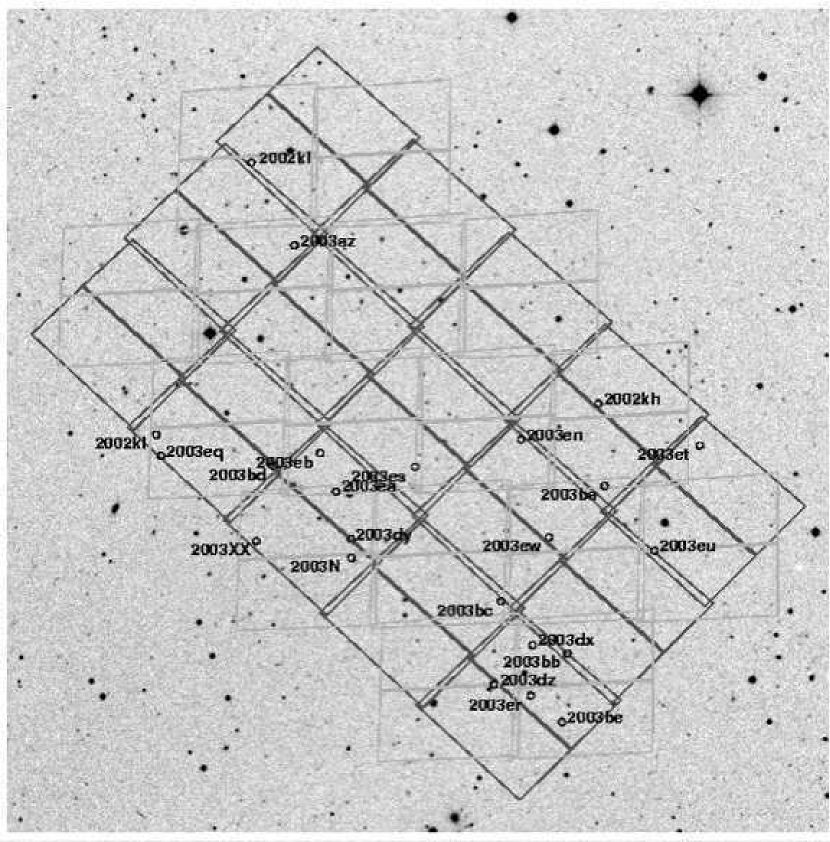
Figure 1: HDFN field observed by the GOODS project. North is up, and east is to the left. The tiles show the ACS pointings for the first (dark) and second (grey) epochs. Epochs 3 and 5 are rotated by $90^{\circ}$ and $180^{\circ}$ (respectively) relative to epoch 1. Epoch 4 is rotated by $90^{\circ}$ relative to epoch 2. The SNe discovered in this field are marked and labeled.

GOODS was designed to combine extremely deep multi-wavelength observations to trace the galaxy formation history and the nature and distribution of light from star formation and active nuclei (Giavalisco et al., 2004a). Using HST/ACS, it has probed the rest-frame ultraviolet (UV) to optical portion of high-redshift galaxies through observations in the $F435W$, $F606W$, $F775W$, and $F850LP$ bandpasses, with a goal of achieving extended source sensitivities only 0.5–0.8 mag shallower than the original Hubble Deep Field observations (Williams et al., 1996). Images were obtained in 15 overlapping “tiled” pointings, covering a total effective area of $\sim 150$ square arcmin per field. Two fields with high ecliptic latitude were observed, the Chandra Deep Field South (CDFS) and the Hubble Deep Field North (HDFN), to provide complementary data from missions in other wavelengths (Chandra X-ray Observatory, XMM-Newton, Spitzer Space Telescope) and to allow ground-based observations from both hemispheres (see Figures 1 and 2).

The GOODS observations in the $F850LP$ band were scheduled over 5 epochs separated by $\sim 45$ days to accommodate a “piggybacking” transient survey. This baseline is ideal for selecting SNe Ia near peak at $z\approx 1$, and SNe Ia on the rise at $z>1.3$, as the risetime (from explosion to maximum brightness) for SNe Ia is $\sim 20$ days in the rest frame (Riess et al., 1999). The baseline also insures that no SN in the desired redshift range will have sufficient time to rise within our detection threshold, and then fall beyond detection before the field is revisited, maximizing the overall yield.

Intentionally, the GOODS filter selections were nearly ideal for the detection, identification, and analysis of high-redshift SNe Ia. For a SN Ia at $z\approx 1$, the $F850LP$ band covers nearly the same part of the SED as the rest-frame $B$ band. The K-correction, or the correction of the observed flux to some rest-frame bandpass (e.g., $F850LP$ to $B$), is thus relatively small.

Monte Carlo simulations of the survey, assuming detection limits based on the $\sim 2100$ s exposure times per epoch (using the ACS Exposure Time Calculator) and the desired baseline between epochs, implied that the distribution of SNe Ia would be centered at $z\approx 1$, with $\sim 1/3$ to $1/2$ of the events occurring in the $1<z<2$ range. Scaling from other lower-$z$ SN survey yields, it was expected that a total of 30–50 SNe of all types would be discovered, and that $\sim 1/2$ of them would be SNe Ia. These numbers implied that we could expect to find $\sim 6$ to 8 SNe Ia in the range of $1.2\lesssim z\lesssim 1.8$, which could be sufficient for an initial investigation of cosmology in the deceleration epoch.

2.1 Image Processing and Search Method

The success of this survey has been due, in large part, to the rapid processing and delivery of data, and the rapid post-processing by a reliable pipeline. The exposures constituting a single tile in a single passband arrived from HST within 6 to 18 hours after observation (with an average of $\sim 10$ hours), and fully processed (differenced with previous epochs) within a few hours after arrival. In general, the complete multi-wavelength data for a single tile were fully searched for candidate SNe within a day after observation.

The individual exposures of a tile in a given epoch were reduced (bias-subtracted and flat-field corrected) through the calacs standard ACS calibration pipeline. The well-dithered subexposures (or CR splits; see below) were then corrected for geometric distortions and combined using the multidrizzle pipeline (Koekemoer et al., 2002). For the survey, we maintained the physical pixel size of $0.05^{\prime\prime}$ pixel^-1 for the discovery of transients.

A key feature of this pipeline is its identification and removal of cosmic rays (CRs) and hot pixels. Each 2100 s exposure in $F850LP$ consisted of 4 individual 520 s CR splits, each dithered by small offsets. In each of the CR splits, the CR contamination, at the time of the survey, was as high as $\sim 1\%$ of all pixels, and hot pixels accounted for an additional $\sim 1\%$ (Riess, 2002). With such a high incidence of CRs and hot pixels, averaging (or taking the median) over the few CR splits would not adequately remove these potential confusion sources. Instead, we used the minmed algorithm described in Mack et al. (2003). Basically, of the pixels in each CR split covering the same area of sky, the highest-value pixel was rejected. The median of the remaining three pixels was then compared to the minimum-value pixel. If the minimum pixel was within 6$\sigma$ of the median, then the median value was kept, otherwise the minimum value was used. A second pass was performed, repeating the minmed rejection on pixels neighboring those which had been previously replaced with minimum values (indicating CR or hotpixel impact), but at a lower threshold to remove “halos” around bright CRs. The result was that each pixel of the output combined image was either the median or the minimum of the input values. Admittedly, the combined result was less sensitive than can be obtained in a straight median, but the multidrizzle algorithm (with minmed) did successfully reject $>99\%$ of CRs and hot pixels after combination.

The search was conducted in 8 campaigns (4 campaigns for each of the HDFN and the CDFS surveys) by differencing images from contiguous epochs. For a given tile in a field, images covering the same area from the previous epoch were aligned (registered) using the sources in the tiles. Catalogs of the pixel centroids and instrumental magnitudes of sources on each image were made using SExtractor (Bertin & Arnouts, 1996) and fed into a triangle matching routine (starmatch, courtesy of B. Schmidt) which determined the linear registration transformation from one epoch to the next. The typical precision of the registrations was 0.2–0.3 pixels root-mean square (RMS), and the point-spread function (PSF) in each epoch of observation remained nominally at 0.10–$0.13^{\prime\prime}$ FWHM. The combination of precise registration and nearly constant PSF allowed for images to be subtracted directly, without the need for image convolution.

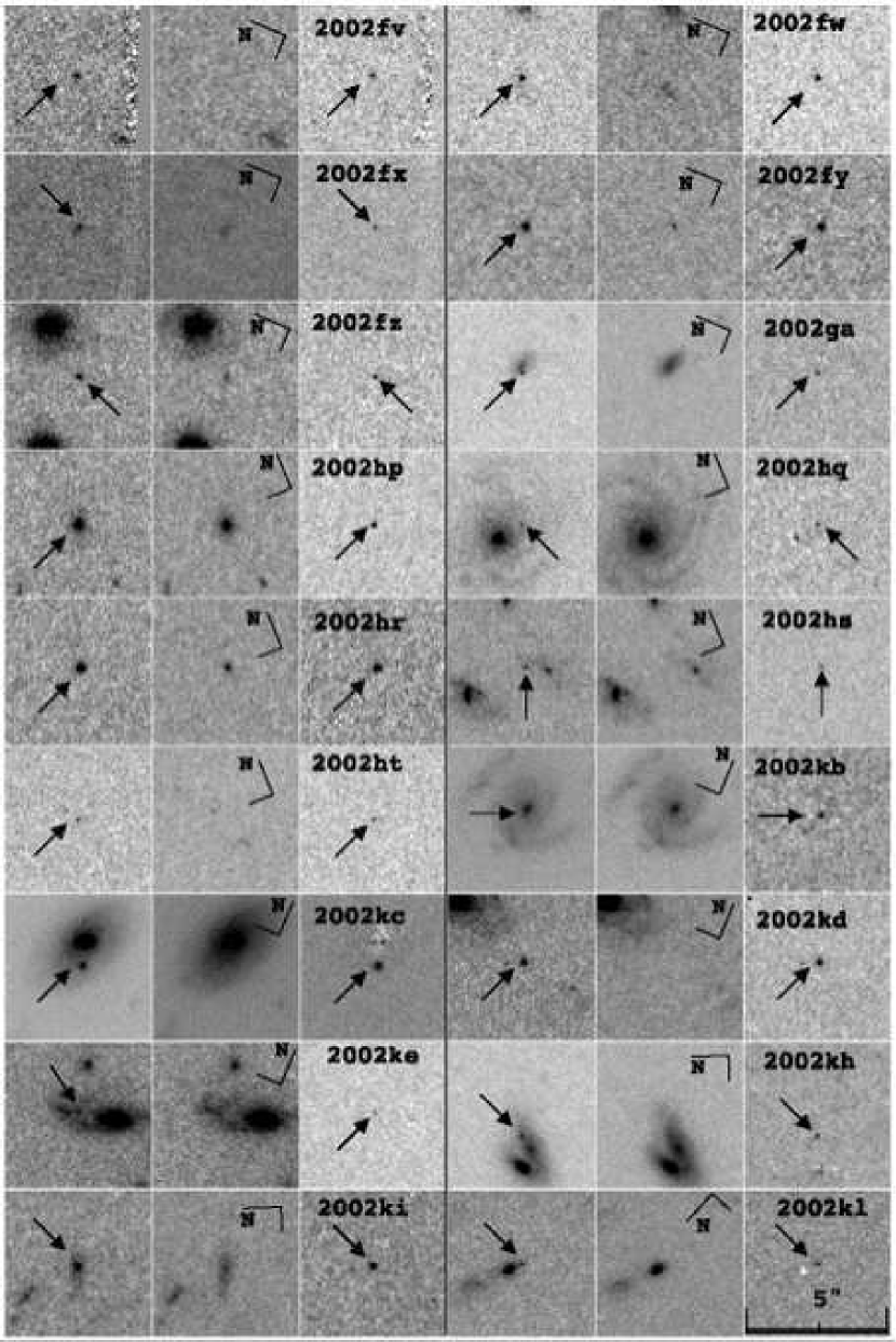
Figure 3: Discovery images for SN 2002fv through SN 2002kl. Each SN has three panels: the discovery image (left), a template constructed from images without the SN (middle), and the subtraction of the two (right). The SN is labeled in the subtraction image. Arrows indicate the position of each SN in the discovery and subtraction images. North and east are marked. The image scale is shown in the lower right-most image.

Several examples of the image subtraction quality are shown in Figures 3, 4, and 5. In ideal situations, only transient sources remain in the residual image on a nearly zero-level background. However, in practice there were many situations which produced non-transient residuals. Although extensive care was taken to remove many CRs and hot pixels in the image processing, these artifacts did occasionally slip past the rejection algorithms, specifically when multiple effects were coincident on the same area of sky. For example, for a given pixel in each of the four CR splits covering the same area of sky, the probability that the pixels were impacted by a CR in 3 of the 4 exposures is approximately 1 in $10^{6}$. Roughly 20 pixels in the combined 20 million pixel array would show CR residuals after passing through the multidrizzle algorithm. In addition, “breathing” in the optical path, focus drift, and the slight change in the pixel scale across the image plane have all led to small yet detectable variations in the PSF. Sometimes bright compact objects were over-subtracted in the wings of their radial profiles and under-subtracted in the inner 1–2 pixels. Other instrumental sources of confusion include diffraction spikes, correlated noise from multiple image resampling, and slight registration errors due to the lack of sources over a large registration area.

The non-trivial abundance of false positives required rigorous residual inspection methods. We therefore searched the subtracted images redundantly to minimize false detection biases and to maximize recovery of elusive, faint transients. An automated routine was performed to identify PSF-like residuals which were well separated ($\geq 2$ pixels) from known saturated pixels, and above $\sim 4-5\sigma$ of the sky background. The inherent nature of this routine prohibits the detection of nonstellar residuals, faint residuals, residuals near bright stars or nuclei (which may be saturated), or residuals in areas where the RMS of the background could not be easily determined by the automated routine. Therefore, so that no potential SNe were lost, several human searchers visually inspected each subtracted image. At least two pairs of searchers independently scoured a few residual tiles. Visual searching of only a few tiles insured that it was done thoroughly, and helped to alleviate monotony and fatigue.

Candidate SNe found by the software and the searchers were then scrutinized based on the following set of criteria to select SNe and further reject instrumental (and astronomical) false positives:

(1) Misregistration: Areas with $\lesssim 10$ detectable sources per arcmin² are typically poorly registered ($\gtrsim 0.5$ pixel RMS). Sources in these areas of the subtracted images are under-subtracted on one side, and over-subtracted on the other. If the total flux in an aperture encompassing the source was not significantly greater than a few times the background RMS, it was assumed that the residual was an artifact of misregistration.

(2) Cosmic ray residuals: The number of pixels in $\sim 2100$ s combined images that still contain CRs due to impacts on the same regions of sky on one or more individual $\sim 520$ s exposures is roughly $4500^{2}\times(0.01)^{N}$, where $N$ is the number of impacted exposures (out of 4). This number can grow slightly when considering hot pixels and bright pixels with CRs. To further reject these artifacts, we required that candidates have no more than one constituent exposure affected by CRs or hot pixels.

(3) Stellar profile: Residuals in the subtracted images were required to show a radial profile consistent with the PSF ($\sim 2$ pixels FWHM). Narrower profiles were considered to be stacked noise (if not residual CRs) and wider profiles were typically poor subtractions from misregistrations, breathing, or focus drift.

(4) Multiple epochs of detection: It was required that each candidate be detected (to within 5$\sigma$) on each of the CR split exposures that were not impacted by CRs or hot pixels at the relevant location. Additional weight was given to candidates that were clearly detected in the $F775W$ band, or additionally in the $F606W$ band. However, this was not a strict criterion as it was expected that SNe Ia at higher redshifts would become less detectable in the bluer wavelengths (see Section 2.2).

(5) Variable galactic nuclei: Sources that were $\lesssim 1$ pixel from their host nuclei were considered potential active galactic nuclei (AGNs) and typically not included in the target of opportunity follow-up program (see §2.3). However, these residuals were followed over subsequent search epochs, and in all but one case, sufficient photometric evidence (see §2.2) was found to classify them as SNe. Bright residuals that were coincident with the nuclei of galaxies were also compared with known X-ray sources from the Chandra Deep Field South and Chandra Deep Field North 1 Megasecond catalogs (Brandt et al., 2001; Giacconi et al., 2002). Indeed, the only variable source unidentified by spectroscopic or photometric means was identified as known X-ray source, and therefore rejected as the only confirmed optically variable AGN in the survey.

(6) Solar-system objects and slow-moving stars: We required that our candidates show no proper motion. Assuming we were sensitive to 1/2-pixel shifts, the proper motion of any candidate could not be more than $0.025^{\prime\prime}$ over the $\sim 2100$ s combined exposure, or $\omega<0.043^{\prime\prime}$ hr^-1 (0.1 deg yr^-1). Hypothetically, if a source was bound to the Sun (with tangential velocity $\sim 30$ km hr^-1), then its distance would have to be $D>$ [(30 km s^-1)/(0.043” hr^-1)], or greater than $3,400$ AU. In addition, if the object was illuminated by reflected sunlight, then its apparent magnitude ($m$) would be related to its angular diameter ($\theta$) by

$$m=m_{\odot}+5\log(\theta/2D),$$ (1)

where $m_{\odot}$ is the apparent magnitude of the Sun. Since $\theta$ must be consistent with the PSF ($\sim 0.1^{\prime\prime}$), the source would have to be $\sim 4$ times larger than Jupiter (at the distance assumed from the limits on proper motion), and the apparent magnitude of the source would have to be $m\approx 55$ mag! Alternatively, using the limiting magnitude for the survey, $m_{\lim}\approx 26$ (see § 4.2), the source would have to have an angular size of $\theta>18^{\circ}$ in order to have been lit by the Sun at its assumed distance.

A similar argument can be made for slow-moving stars. Since $\omega=0.043^{\prime\prime}$ hr^-1 is the fastest a source could move without being detected, in the $\sim 45$ days since the field was last observed the source could have moved $<1000$ pixels. Our survey was clearly sensitive to negative residuals as well as positive ones (a fact indicated by the frequent discovery of SNe declining in brightness since the previous epoch). We saw no negative candidates which were detected within 1000 pixels of a positive source on the same epoch of observation.

Most of these SNe have been observed on more than one epoch, and all but two were detected within $3.5^{\prime\prime}$ of a galaxy (presumably the host). It would be highly unlikely for any of these to be objects moving within the Solar System or the Galaxy.

2.2 Identification of SNe and Redshift Determination

SNe are generally classified by the presence or absence of particular features in their optical spectra (see Filippenko 1997 for a review). Historically, the primary division in type has been by the absence (SNe I) or presence (SNe II) of hydrogen in their spectra, but the classification currently extends to at least 7 distinct subtypes (SN IIL, IIP, IIn, IIb, Ia, Ib, and Ic). It is now generally accepted that the explosion mechanism is a more physical basis by which to separate SNe. SNe Ia probably arise from the thermonuclear explosion of carbon-oxygen white dwarf stars, while all other types of SNe are produced by the core collapse of massive stars ($\gtrsim 10M_{\odot}$).

There can be considerable challenges in the ground-based spectroscopic identification of high-redshift SNe. As the principal goal of this survey has been to acquire many SNe Ia at $z>1$, a fundamental prerequisite was that we could make confident identifications of at least this SN type. Much to our benefit, HST with the ACS $G800L$ grism provides superb spectra with significantly higher signal-to-noise ratio (S/N) than can currently be achieved from the ground. Its limitation is the low spectral resolution ($R\equiv\lambda/\Delta\lambda\approx 200$ per pixel, in first order) and the overlap of multiple spectral orders from other nearby sources. Spectral resolution of $\sim 1500$ km s^-1 is not problematic for SNe with ejecta velocities of $\gtrsim 10,000$ km s^-1. However, because of the spectral-order confusion and the lack of a slit mask, the $G800L$ grism could only be used for SNe with substantial angular separation from their hosts and from other nearby sources.

It was expected that SN candidates would generally be either too faint to be spectroscopically observed from the ground, or too close to their host galaxies or other nearby sources to be identified with the ACS grism. We therefore had to rely on some secondary method by which to identify SNe, specifically to select likely SNe Ia from the sample. The inherent differences in the ejecta compositions of SNe Ia and SNe II leads to an observable difference in their intrinsic early-time UV flux. As optical observations shift to the rest-frame UV for $z\gtrsim 1$ SNe, the “UV deficit” in SNe Ia can be a useful tool for discriminating SNe Ia from SNe II, the most common types of core-collapse (CC) SNe. Using a method pioneered by Panagia (2003) and fully developed in Riess et al. (2004b), we use the $F850LP$ apparent magnitude, the $F775W-F850LP$ and $F606W-F850LP$ colors, the measured redshift or photometric redshift estimates (see below), and age constraints provided by the baseline between search epochs to grossly identify SNe as either SNe Ia or SNe CC. This method is only useful for $z\gtrsim 1$ SNe near maximum light, and is not foolproof in its identification. There are SNe CC (e.g., luminous SNe Ib and Ic) which can occupy nearly the same magnitude-color space as SNe Ia. However, these bright SN Ib/c make up only $\sim 20$% of all SNe Ib/c, which as a group are only $\sim 1/3$ as plentiful as other SNe CC (Cappellaro, Evans, & Turatto, 1999).

From the ground, we have obtained spectroscopic identification of 6 SNe Ia and 1 SN CC in the redshift range 0.2–1.1 using Keck + LRIS (see Table 1). With HST/ACS and the $G800L$ grism, we have obtained excellent spectra of 6 SNe Ia at $z=0.8$–1.4, the most distant sample of spectroscopically confirmed SNe; see Riess et al. (2004a). These spectra cover only the 2500–5000 Å range in the rest frame, but they are of excellent S/N, unattainable for such high-$z$ SNe from the ground. These identifications also serve as an excellent proof of concept in the color-magnitude selection.

Using Keck, the VLT, and the ACS grism, we have obtained spectroscopic redshifts for 29 of the 42 SNe in our sample. To our benefit, part of the GOODS endeavor involved obtaining extensive multi-wavelength photometry spanning the $U$ to the near-IR passbands to estimate the photometric redshifts (“phot-$z$”) of galaxies in the HDFN and CDFS fields (Mobasher et al., 2004). The precision of the phot-$z$ from GOODS with respect to known spectroscopic redshifts has been within $\sim 0.1$ RMS, with the occasional instance ($\sim 10\%$ of a tested sample) where the phot-$z$ method misestimates the actual redshift by more than 20%. In order to improve on the accuracy of the phot-$z$ measurements for the host galaxies, we remeasured the multi-wavelength photometry by visually determining the centroid of the host galaxies, and manually determining an annulus in which the sky background is determined. This allowed better photometric precision than was generally achieved in the SExtractor-based automated cataloging. Comparing the sample of 26 SN host galaxy spectroscopic redshifts to the phot-$z$ estimates from the improved photometry resulted in a precision of 0.05 RMS (after rejecting two $>7\sigma$ outliers), and only $\sim 5\%$ of the sample was misestimated by more than 10% (see Figure 6). The redshifts of the remainder of the SN hosts (without spectroscopic redshifts) were determined in this way, with the exception of SN 2002fv, whose host was not identified due to the magnitude limits of the survey.

We fit template light curves to grossly identify SNe which were not spectroscopically identified, and were not at $z\gtrsim 1$ nor constrained near maximum light. Using the light curves of SNe 1994D, 1999em, 1998S, and 1994I as models for SNe Ia, IIP, IIL, and Ib/c (respectively), we transformed these model SNe to the redshifts of the observed SNe, correcting for the effects of time dilation, and applying K-corrections to the rest-frame bandpasses to produce light curves as they would have been seen through the $F850LP$, $F775W$, and $F606W$ bandpasses at the desired redshifts. The K-corrections were determined from model spectra (Nugent, Kim, & Perlmutter, 2002) for SNe Ia, and from color-age light-curve interpolations for SNe CC. We have also made use of the web tool provided by Poznanski et al. (2002) to check the derived colors for the SNe CC. We visually determined the best-fit model light curve to the observed light curves, allowing shifting along the time axis, magnitude offsets, and extinction/reddening (assuming the Galactic extinction law) along the magnitude axis. Best fits required consistency in the light-curve shape and peak color (to within magnitude limits) and in peak luminosity in that the derived absolute magnitude in the rest-frame $B$ band had to be consistent with the observed distribution of absolute $B$-band magnitudes shown in Richardson et al. (2002).

Each discovered SN was given an identity rank (gold, silver, or bronze) reflecting our confidence in the identification. A gold rank indicated the highest confidence that the SN was the stated type, and it was not likely that the SN could have been some other SN type. A silver rank indicated the identity was quite confident, but the SN lacked sufficient corroborating evidence to be considered gold. A bronze rank indicated that there was evidence the SN type was correct, but there was a significant possibility that the SN type was incorrect.

We were clearly confident of the SN type in cases where a high S/N ($\gtrsim 20$) spectrum conclusively revealed its type; these SNe were gold, by definition. However, the majority of SNe were without sufficient spectra to unambiguously determine a type. We then used additional information on the SN redshift, photometric data, and host-galaxy morphology, seeking a consistent picture for a specific SN type.

We first considered the possibility that a candidate was a SN Ia. We required that the light-curve shape was at least consistent with a SN Ia at its redshift, and that the observed colors and derived absolute magnitude could be made consistent with the template light-curve colors with $<1$ mag of extinction (assuming the Galactic extinction law). If the SN was at $z\gtrsim 1$, and its peak colors were $F775W-F850LP\gtrsim 0.5$ mag and $F606W-F850LP\gtrsim 1$ mag, we considered it highly likely to be a SN Ia.

The study of Hamuy et al. (2000) has shown that at low redshifts, early-type galaxies (ellipticals) only produce SNe Ia, and have not as yet been shown to produce SNe CC. Hence, we regard SNe found in red elliptical hosts to have been most likely SNe Ia and unlikely SNe CC.

Based on the above information, any SN in our survey at $z>1$, in a red elliptical host, and having light curves and peak colors consistent with a SN Ia, were most confidently considered SNe Ia and ranked “gold SNe Ia.” SNe having photometric data consistent with SNe Ia, and either at $z>1$ (identifiable by their peak color) or in early-type host galaxies, were considered SNe Ia with a high confidence, and therefore ranked “silver SNe Ia.” SNe having light curves consistent with SNe Ia, but without any other information to confirm their type, were ranked as “bronze SNe Ia.”

If the light curves for a SN seemed inconsistent with a SN Ia, we compared them to the model light curves for SNe CC. If the SN showed a slow rate of decline from peak (consistent with SNe IIP and some SNe IIn), then it was considered a SN CC with high confidence, or a “silver SN CC.” All other SNe, inconsistent with SNe Ia, SNe IIP, or slowly declining SNe IIn, were placed into the “bronze SN CC” category. For clarity, we include a flow chart showing the conditions used to determine the identification confidence rank (Figure 7).

2.3 Follow-up HST Observations

An intensive target of opportunity (ToO) follow-up program with HST (GO 9352; Riess, PI) was conducted for candidate SNe Ia in the range of $z\gtrsim 1$. The decision to trigger the ToO was based on the prior certainty of SN Ia type and redshift range. These observations are intended to support multi-wavelength light-curve shape fitting (Riess et al., 1996) with multiple observations in passbands as close to the rest-frame $U$, $B$, and $V$ bands as possible. The ToO program consisted of supplementary observations with ACS (in $F775W$ and $F850LP$ bands), NICMOS (in the $F110W$ and $F160W$ bands), and ACS $G800L$ grism spectra when feasible. These observations were rapidly initiated (within $\sim 1$ week of SN detection) so that identification and color measurements could be made as near to maximum light as possible, and so that the light-curve sampling could be optimized. Using an updated version of the multicolor light-curve shape algorithm (Jha, Riess, & Kirshner 2004, in preparation), we estimate key parameters of the rest-frame optical light curves, particularly the $B$-band magnitude at maximum, the rest-frame $U-B$ and $B-V$ colors at maximum, and the rate of decline from maximum light in the $B$ band. Further details on the ToO program, including the photometric and spectroscopic data, can be found in Riess et al. (2004b).

3 Results of the Survey

Over the course of 8 search campaigns from 2002 August to 2003 May, we successfully discovered 42 SNe of both physical types over a wide range of redshifts. The SNe are shown in their discovery-epoch images in Figures 3, 4, and 5. They are listed in Table 1 with their U. T. date of discovery, coordinates, physical SN type, type confidence, redshift, source of measured redshift, and offset from host galaxies, if detected.

The optical HST/ACS photometry for most of the SNe is given in Table 2. This photometry consists of discovery epoch apparent magnitudes, and data on the SN (when detected) from subsequent search epochs. The optical and infrared photometry for the 16 SNe Ia which were used in the cosmological analysis (specfically SNe 2002fw, 2002fx, 2002hp, 2002hr, 2002kc, 2002kd, 2002ki, 2003ak, 2003az, 2003bd, 2003be, 2003dy, 2003eb, 2003eq, 2003es, and 2003lv) are shown in Riess et al. (2004b). The data listed in Tables 1 and 2, and in Riess et al. (2004b), supersede preliminary data announced in IAU Circulars 7981, 8012, 8038, 8052, 8069, 8081, 8083, 8125, 8140, and 8141.

For each SN, images from all survey epochs in which the SN was not detected (to within a 10$\sigma$ limit) were combined to create a template image. Images from each epoch in which the SN was detected had the template image subtracted from it to remove the host galaxy and other background light. The apparent magnitude in each passband was measured through a narrow aperture ($0.15^{\prime\prime}$ radius) centered on the SN. The residual sky brightness (and noise) were determined in larger aperture annuli (0.6–1^′′). Aperture corrections determined by Gilliland & Riess (2002) were applied to correct from the encircled flux in the narrow aperture to what would be expected in a nearly infinite aperture. We then measured the apparent magnitudes relative to the 1 count per second zero points determined by Sirianni et al. (2003). Photometric errors were approximated using the ACS Exposure Time Calculator.

4 Delay Time Functions and Models for SNe Ia Progenitor Systems

The current consensus on SNe Ia is that they are thermonuclear explosions of white dwarf (WD) stars as they accrete matter to reach the Chandrasekhar mass (Livio, 2001). The two most likely scenarios are single degenerate (SD) systems (a single WD accreting material from a normal companion star), and double degenerate (DD) systems (the merger of two WDs). It is not yet fully understood which scenario represents the preferred mechanism or channel for the production of these events, or if more than one channel is used by progenitors to make SNe Ia. To that end, there is some uncertainty concerning the characteristic time scale from the formation of these progenitors to the occurrence of the events, and concerning the distribution of these delay times. Nevertheless, there is some consensus that the delay time in the SD scenario is chiefly governed by the main-sequence lifetime of the companion star which is on the order of 10⁹ yr, and in DD by the time necessary to gravitationally radiate away the angular momentum (Iben & Tutukov, 1984; Tutukov & Yungelson, 1994) which is on the order of 10⁸ yr. Chemical evolution in the solar neighborhood (Yoshii, Tsujimoto, & Nomoto, 1996), and additional SD/DD modeling  (Ruiz-Lapuente & Canal, 1998; Hachisu et al., 1999), suggest 0.5–3 Gyr mean delay times should be plausible for SD, and a mean of $\sim 0.3$ Gyr in DD.

Even within the SD scenario, there is quite a diversity of specific models. In addition to the substantial mass accretion [$\dot{M}_{acc}\approx(5-10)\times 10^{-8}$ M_⊙ yr^-1], there can be significant winds ($\dot{M}_{wind}\approx-0.5\dot{M}_{acc}$), and possibly companion-mass stripping ($\dot{M}_{strip}\approx-0.1\dot{M}_{acc}$) to accommodate a larger range in companion star masses (Hachisu et al., 1999). Indeed, there are a variety of SD models which can reproduce a satisfactory set of SN Ia characteristics, but none as yet which have thoroughly accounted for the SN Ia diversity (see Livio 2001 for a review). It is possible, in light of this diversity, that there are several channels by which SNe Ia are produced. For example, it is possible to imagine a scenario in which SD channels account for the majority of SN Ia events, perhaps $\gtrsim 80\%$, and the other $\sim 20\%$ would come from DD systems. This would be consistent with the observed luminosity diversity at $z\approx 0$, and, assuming some simple evolutionary arguments, could account for the apparent lack of diversity at higher redshifts (Livio, 2001; Li et al., 2001). Ultimately, it is this uncertainty in the progenitor systems that inevitably makes it difficult to quantify the intrinsic distribution of delay times, which would allow a comparison of the observed SN Ia rate to the star formation rate.

We therefore attempt to constrain the apparent distribution of delay times through the observed SN rates and measurements of the star formation history. The frequency distribution, or number distribution [$N_{Ia}(z)$], of SNe in our survey can be given by

$$N_{Ia}(z)=\text{SNR}_{Ia}(z)\times t_{c}(z)\times(1+z)^{-1}\times\frac{\Theta}{4\pi}\times\Delta V(z),$$ (2)

where SNR${}_{Ia}(z)$ is the intrinsic SN volume rate (number per unit time per unit comoving volume). The survey’s efficiency with redshift is represented as a “control time,” $t_{c}(z)$, or the amount of time in which a SN Ia at a given redshift could have been observed by our survey (see § 4.2). $\Theta$ is the solid angle of the survey area ($\sim 300$ sq. arcmin, or $2.54\times 10^{-5}$ steradians). $\Delta V$ is the volume comoving element contained in a shell about $z$ and is defined by $\Delta V(z)\equiv V(z+\Delta z)-V(z)$, with

$$\begin{split}V(z)=&4\pi H_{0}^{-3}(2\Omega_{k})^{-1}\\ &\times\biggl{\{}H_{0}\biggl{(}\frac{D_{L}(z)}{1+z}\biggr{)}\biggl{[}1+\Omega_{k}H_{0}^{2}\biggl{(}\frac{D_{L}(z)}{1+z}\biggr{)}^{2}\biggr{]}^{1/2}\\ &-|\Omega_{k}|^{-1/2}sinn^{-1}(H_{o}\biggl{(}\frac{D_{L}(z)}{1+z}\biggr{)}|\Omega_{k}|^{1/2})\biggr{\}},\end{split}$$ (3)

where $H_{0}$ is the Hubble constant at the present epoch $t_{0}$, and $D_{L}$ is the luminosity distance. Here “$sinn$” and $\Omega_{k}$ are terms which describe the curvature of space, where $sinn=sinh$ when $\Omega_{k}>0$ (open Universe), and $sinn=sin$ when $\Omega_{k}<0$ (closed Universe). $\Omega_{k}$ is defined by $1-\Omega_{k}=\Omega_{M}+\Omega_{\Lambda}$.

We assume that the intrinsic SN Ia rate would be a reflection of the star formation rate, SFR$(z)$, distorted and shifted to lower redshifts by the convolved delay time distribution function, $\Phi(t_{d})$:

$$\text{SNR}_{Ia}(t)=\nu\int_{t_{F}}^{t}\text{SFR}(t^{\prime})\times\Phi(t-t^{\prime})~{}dt^{\prime},$$ (4)

where $\int\text{SNR}_{Ia}(z)~{}dz\equiv\int\text{SNR}_{Ia}(t)~{}dt$. Here, $t$ is the age of the Universe at redshift $z$, $t_{F}$ is the time when the first stars were formed, and for computational convenience, we set $z_{F}=10$. We define $\nu$ as the number of SNe Ia per formed solar mass. Therefore, $\Phi(t_{d})$ is the frequency distribution of SNe Ia (yr^-1), and represents the relative number that explode at a time $t_{d}$ since a single burst of star formation.

As the HHZSS$-$GOODS data span a vast range in redshift extending to $z\approx 1.6$, they are well suited to probing SNR${}_{Ia}(z)$, and to determining $\Phi(t_{d})$. In this analysis, we attempt to determine constraints on $\Phi(t_{d})$ by testing a few model distributions in their ability to recover the observed redshift distribution of SNe Ia from this survey. Overall normalization factors, such as the number of SNe per unit formed stellar mass, are largely ignored in this analysis. The actual rates of SNe Ia (including normalization) are calculated and analyzed in Dahlen et al. (2004). We use the gold, silver, and bronze SNe Ia together (a total of 25 SNe Ia) throughout this analysis, and we assume $\Omega_{M}=0.30$, $\Omega_{\Lambda}=0.70$, and $H_{0}=70$ km s^-1 Mpc^-1.

4.1 The Star Formation Rate Model

Various observations of galaxies in the rest-frame passbands have given information on SFR$(z)$, now extending to $z\gtrsim 5$ (Giavalisco et al., 2004b). This current model broadly supports the findings of Madau, Pozzetti, & Dickinson (1998) in suggesting that SFR$(z)$ is peaked at $1<z<2$, but it is substantially flatter in its decline at $z>2$. There is, however, some uncertainty in the amount of correction for extinction in the galaxies themselves (see Giavalisco et al. 2004b for a discussion). Indeed, without the extinction correction, the deduced SFR$(z)$ would be similar to the Madau, Pozzetti, & Dickinson (1998) function, but extending to higher redshifts.

We therefore chose to include an analysis for two SFR models. Using a modified version of the parametric form suggested by Madau, Della Valle, & Panagia (1998), we assume SFR$(t)$ evolves as

$$\text{SFR}(t)=a(t^{b}e^{-t/c}+d~{}e^{d(t-t_{o})/c}),\\$$ (5)

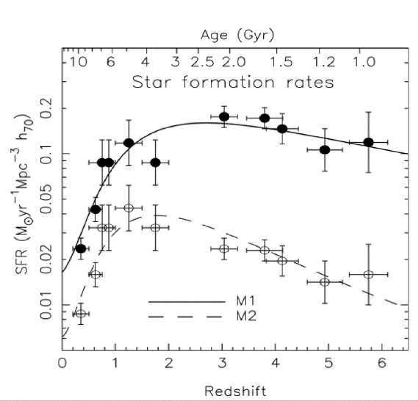
Figure 8: The star formation rate history models (M1 and M2), shown relative to measurements of the star formation rate at various redshift intervals.

where $t$ is given in Gyr. By fitting the measurements of SFR$(z)$ from several surveys (see Giavalisco et al., 2004b), we determined the coefficients of the function to be $a=0.182,~{}b=1.26,~{}c=1.865,~{}\text{and}~{}d=0.071$ for the extinction-corrected model (M1), and $a=0.021,~{}b=2.12,~{}c=1.69,~{}\text{and}~{}d=0.207$ for the uncorrected model (M2; see Figure 8). Here $t$ is the age of the Universe at redshift $z$, and $t_{o}=13.47$ corresponds to $z=0$ for both models.

4.2 The Control Time: The Efficiency of the Survey

In comparing predicted yields to what was observed, it is imperative that corrections are made based on various conditions of the survey. This includes observational effects such as the magnitude limits, effective sky coverage, and time over which the survey was conducted, as well as SN type parameters such as the intrinsic luminosity range, light-curve shapes, and extinction environments. We combine all of these systematic effects to a single parameter, the “control time” [$t_{c}(z)$], which is in effect the amount of time a SN at a given redshift could have been observed. We define $t_{c}(z)$ as

$$t_{c}(z)=\int_{t}\int_{M_{\lambda}}\int_{A_{\lambda}}P(t|M_{\lambda},A_{\lambda},z)P(M_{\lambda})P(A_{\lambda})~{}dA_{\lambda}~{}dM_{\lambda}~{}dt,$$ (6)

which is a product of probabilities for observing a SN of specific absolute magnitude ($M_{\lambda}$, at rest-frame central wavelength $\lambda$) with specific host-galaxy extinction ($A_{\lambda}$) at specific times ($t$), summed over all viable absolute magnitudes, extinction values, and time. All parameters in the equation are dimensionless, except for $dt$ with units of time.

We determined the sensitivity of our survey in a real-time method, by placing false SNe of random magnitudes (in the range 23–27 mag) in search-epoch images. The modified search images passed through our image-subtraction pipeline, on to the visual inspection, unbeknownst to the search team. In doing so, we were able to determine the combination of the intrinsic sensitivity limits and the search team’s efficiency. Only a moderate number ($\sim 40$) of false SNe were added to the survey data so that searchers would not become desensitized to real transients by an overwhelming number of bogus detections. To add some realism to the test, the majority of false SNe were added to known galaxies in a Gaussian radial distribution ($0.50^{\prime\prime}\pm 0.25^{\prime\prime}$, $10\pm 5$ pixels) truncated at zero radius. It has also been documented that in intermediate and high redshift surveys, a few SNe have been discovered without host galaxies, to within the detection limits of these surveys (Strolger et al., 2002; Gal-Yam et al., 2003; Germany et al., 2004; Germany & Strolger, 2004). We therefore placed a few SNe in completely random locations, so that searchers would not bias their discoveries based on the requirement of a host galaxy. Astonishingly, 100% of test SNe were recovered to $m_{F850LP}\leq 25$ mag, a testament to the efficacy of the search team and the unparalleled stability of observing conditions with HST. Beyond $m_{F850LP}\approx 25$ mag, the recovery efficiency drops rapidly, reaching zero at $m_{F850LP}\gtrsim 26.5$ mag.

The limitation of the of this real-time method was that there were few fake SNe, and therefore only a gross range in detection efficiency could be assessed. This test cannot appropriately test both rate of decline in efficiency, and the effects of host galaxy light contamination on the efficiency. We therefore independently tested the sensitivity of the survey through a more thorough Monte Carlo simulation.

500 random host galaxies with phot-$z$ in the range of 1.5 to 2.0 were selected from the GOODS data, and combined to produce light profile of galaxies in this redshift range. A function was fit to the combined light profile using galfit:

$$Bulge =s_{e}\times\exp\biggl{[}-7.688\biggl{(}\frac{r}{r_{e}}^{1/4}-1\biggr{)}\biggr{]}$$ (7)

$$Disk =s_{o}\times\exp\biggr{[}-\frac{r}{r_{o}}+\frac{r_{1}}{r}^{3}\biggr{]}$$ (8)

$$Total =Bulge+Disk+Background,$$ (9)

where the total light profile is well fit by $s_{e}=0.01,\,r_{e}=0.055,\,s_{o}=0.02,\,r_{o}=3.0,\,r_{1}=0.0,$ and $Background\approx 0$. A set galaxies with phot-$z$ from 1.5 to 2.0 (183 total) were selected in two test tiles, and one fake SN with a random magnitude in the range 25.5–27.5 was added to each of these galaxies with a radial distribution which follows the derived cumulative light profile. A second distribution of faint SNe (24 – 26.5 mag) were also added to selected bright galaxies with phot-$z<0.5$ using the same radial distribution as was used for the faint population of galaxies (181 SN total, one per galaxy). These test images were then run through the processing pipeline, and recovered using the automated residual detection algorith. The results of both efficiency tests were combined to produce a histogram of recovered fake SNe as a fraction of the number added (shown in Figure 9).

We fit an analytical function to the efficiency distribution following

$$\varepsilon(\Delta m)=\frac{T}{1+e^{(\Delta m-m_{c})/S}},$$ (10)

where $\Delta m$ is the magnitude corresponding to the flux difference between two consecutive epochs in the $F850LP$ band, determined by

$$\begin{split}m_{1}&=ZP-2.5\times\log(F_{1})\Rightarrow F_{1}=10^{-\frac{2}{5}(m_{1}-ZP)}\\ m_{2}&=ZP-2.5\times\log(F_{2})\Rightarrow F_{2}=10^{-\frac{2}{5}(m_{2}-ZP)}\\ \Delta m&=ZP-2.5\times\log(F_{2}-F_{1}).\end{split}$$ (11)

Here $ZP$ is the photometric zero point, $T$ is the maximum efficiency, $m_{c}$ represents a cutoff magnitude where $\varepsilon(\Delta m)$ drops below 50% of $T$, and $S$ controls the shape of the roll-off. As seen in Figure 9, the real-time tests show a maximum efficiency which remains at 100% ($T=1$) until $\sim 25.5$ mag, where background noise begins to play an important role. $\varepsilon(\Delta m)$ drops with $S=0.4$, reaches the cutoff at $\Delta m_{c}=25.85\pm 0.1$, and is essentially zero at $\Delta m\geq 27$. A weighted least-squares fit to the Monte Carlo data show $T=1.03\pm 0.09$, $m_{c}=25.91\pm 0.12$, and $S=0.39\pm 0.08$. As the maximum efficiency cannot be $>100\%$, we set T=1 as a prior, and found $m_{c}=25.94\pm 0.05$ and $S=0.38\pm 0.06$. It is important to note that $m_{c}$ represents only a $\sim 5\sigma$ cutoff. Our simulations show we could detect SNe to within $\sim 3\sigma$, but only a small fraction of the time (depending on the local background light).

As with other supernova surveys, it was expected that the efficiency would not only depend on the brightness of the SN, but also the brightness of the host galaxy and the local gradient of light (or synonymously the distance from the host nucleus). Most modern surveys use image subtraction methods to find SNe, and therefore generally do not lose SNe because of overall light contamination from the SN environment, as was the case with the original “Shaw Effect” (Shaw, 1979). However, faint SNe are lost in the Poisson noise of the host galaxies (cf. Hardin et al., 2000), or in the residual remaining from an imperfect subtraction of the host galaxy. To account for the possibility of this pseudo-Shaw Effect, we separated the fake SNe into two distributions based on their proximity to the center of the host nuclei, and drew recovery efficiency histograms from the samples (see Figure 10). The efficiency histogram drawn from the fake SNe which were nearly coincident with their host nuclei, with radial distances of less than 5 pixels, showed no substantial difference from the histogram drawn from well-separated SNe, indicating that the Shaw Effect was likely insignificant to this survey. In fact, there was a slight tendency to find more SNe at small radial distances than at larger radial distances. This was an attributed to the automated residual detection algorithm, which also identified the residuals of galaxies due to breathing or focus drift as potential SNe. An important distinction between the real-time method and the Monte Carlo test was that human searchers were capable of distinguishing and rejecting a poor subtraction due to a change in the PSF from a SN candidate, whereas the automated method was not. In reality, regions which showed such PSF residuals were deemed “unsearchable” and rejected.

To asses what fraction of SNe could be lost by rejecting these unsearchable regions (and therefore a potential loss in efficiency), we convolved a test image with a narrow Gaussian filter to produce an image with PSF $\approx 3$ pixels FWHM, which is 5–10% larger than the PSFs recorded under the worst conditions of the survey. This convolved image was subtracted from the original image (without the convolution) to produce galaxy residuals which are under-subtracted in the cores. A histogram was drawn from the 2 pixel aperture magnitudes of these residuals, which is well represented by a Gaussian with $\langle\Delta m\rangle=28.42,\,\,\sigma=0.707$. SNe with magnitudes equal to or less than that of a galaxy residual cannot be distinguished from the residual itself, and therefore the flux contained in the narrow region of the core would be unsearchable for SNe of those magnitudes. Accordingly, this flux cannot be included in the total of galaxy light surveyed. As the SN rate is expected to follow the galaxy light, the rejected flux would result in a loss in the overall number of SNe discovered, which we represent as a reduction in efficiency.

For example, a galaxy core which produced a 22 mag residual would be unsearchable for SNe $>22$ mag. Therefore, the efficiency for SNe $>22$ mag would drop by a fraction proportional to the fraction of all galaxy light that is contained in the cores of galaxies which could produce 22 mag residuals. Fainter galaxy residuals only reduce the efficiency for fainter SNe. These faint galaxy residuals are more numerous, but the flux within the cores of the galaxies which produced them is a considerably smaller fraction of the total flux in the image, and therefore their rejection would result in only a small contribution to the efficiency loss.

We find that only 8% of the total light in an image was contained in the cores of galaxies, nearly half of which resided in bright galaxies. The galaxies which produced residuals $>23$ mag accounted for approximately $4\%$ of the flux in the image, and therefore an overall 4% efficiency reduction for all SNe. Increasingly fainter galaxies further reduced the efficiency for fainter SNe, leading to a 6% efficiency drop by $\Delta m=m_{c}$, and a 8% reduction by $\Delta m=27.5$. As can be seen in Figure 9, the pseudo-Shaw Effect does not significantly reduce the efficiency. As this test involved the worst possible conditions of the survey, it serves only as an upper limit to the impact on the efficiency.

The survey efficiency was used to determine the probability of detecting SNe Ia of all redshifts at any given time [$P(t)$ in eq. 6]. To do so, it was important to use a SN Ia light-curve model that has well observed multi-wavelength data extending to the rest-frame $U$ band. We used SN 1994D (R. C. Smith 2003, private communication), a luminous yet “normal” (cf. Branch, Fisher, & Nugent, 1993) SN Ia with $UBVRI$ observed light curves. Studies have shown that this SN was relatively blue in $U-B$ (by as much as 0.3 mag) compared to normal SNe Ia at early epochs (Poznanski et al., 2002). We therefore attempt to correct for this color excess in the template by applying a linear color correction which is 0.3 mag when the central wavelength of the $F850LP$ filter matches, or is blueward of the rest-frame central wavelength of the $U-$band filter, and gradually decreases to 0.0 mag when the $F850LP-$band matches or is redward of the rest-frame $B-$band. The light curves of SN 1994D were adjusted to the rest frame, and relative to maximum light.

The apparent brightness of a SN Ia depends on a its luminosity, the age of the SN, the filter in which it is observed, its local host extinction, and the distance of the event. For a SN Ia of a given absolute magnitude ($M_{peak}$), redshift [or luminosity distance, $D_{L}(z)$], and extinction ($A_{\lambda}$), we chose intrinsic light curve, $\mathcal{M}_{\lambda}(t^{\prime}_{a})$, of the SN Ia model in the rest-frame passband which most closely matches the observed $F850LP$ band. The apparent $F850LP$ magnitude at any point in the model light-curve was determined by

$$\begin{split}m&{}_{F850LP}(t^{\prime}_{a},z)=M_{peak}+\mathcal{M}_{\lambda}[t^{\prime}_{a}\times(1+z)^{-1}]+(U-B)_{94D}\\ &+K^{\lambda}_{F850LP}[z,t^{\prime}_{a}\times(1+z)^{-1}]+A_{\lambda}+5~{}log(D_{L}(z))+25.\end{split}$$ (12)

We assumed that SNe Ia are nearly homogeneous events, with a luminosity at peak of $M_{peak,B}=-19.5\pm\Delta M_{peak}$. The $(U-B)_{94D}$ parameter corrects for the for the U-B color of the template (as described above), and $K^{\lambda}_{F850LP}$ is the K-correction from the rest-frame bandpass to the $F850LP$ band. $t^{\prime}_{a}$ is the modified age of a SN Ia relative to the epoch of maximum light in the $B-$band (see below). We further assumed the intrinsic $B-V$ color of SNe Ia at peak is 0.0 (Lira, 1995).

It has been shown that there is a dispersion in peak absolute magnitudes of SNe Ia, and that the relative peak luminosity of the events relates to the rate in which their light curves evolve from maximum light. Luminous SN 1991T-like SNe Ia decline in brightness more slowly than more normal SNe Ia, and under-luminous SN 1991bg-like SNe Ia fade more rapidly from peak brightness. Several methods have been developed to account for this relation, e. g. the $\Delta M_{15}(B)$ method (Phillips, 1993), the “stretch” method (Perlmutter et al., 1997), and the multicolor light-curve shape algorithm (Riess et al., 1996). To account for the heterogeneity of SN Ia peak luminosity, and the corresponding effect on the light-curve evolution, we used a combination of the most recent adaptation of $\Delta M_{15}(B)$ method (Phillips et al., 1999) and the stretch method (Perlmutter et al., 1997). The $\Delta M_{15}(B)$ parameter is related to the peak luminosity by the Phillips et al. (1999) relation,

$$\Delta M_{peak}=0.786(\Delta m_{15}(B)-1.1)+0.633(\Delta m_{15}(B)-1.1)^{2},\\$$ (13)

which is well suited for SNe Ia in the range of $0.7<\Delta M_{15}(B)<1.7$, extending from the most luminous and slowly declining, to the less luminous, yet normal SNe Ia. However, it does not appropriately account for the SNe Ia similar to SN 1991bg, which evolve very rapidly and are intrinsically several magnitudes fainter than SNe Ia in the normal range. Indeed, the Phillips et al. (1999) relation is $\sim 1.5$ magnitudes brighter in the $B-$band than has been observed for SN 1991bg-like SNe in the range $1.7<\Delta M_{15}(B)<2.2$. We therefore applied a correction to the relation for SNe Ia in this range of $\Delta M_{15}(B)$,

$$\Delta M_{peak}=1.35+0.786(\Delta m_{15}(B)-1.1)+0.633(\Delta m_{15}(B)-1.1)^{2}.$$ (14)

Li et al. (2001) have found that the distribution of SNe Ia favors normal events, with only $\sim 20\%$ of events in the range $0.7<\Delta m_{15}(B)<0.9$ (SN 1991T-like SNe), about 20% in the $1.7<\Delta m_{15}(B)<2.2$ range (SN 1991bg-like SNe), and the remaining 60% in the $0.9<\Delta m_{15}(B)<1.7$ range. We attempted to characterize this observed distribution by assuming the intrinsic dispersion in $\Delta M_{15}(B)$ is Gaussian, centered at $\Delta M_{15}(B)=1.1\pm 0.35$ and truncated at $\Delta M_{15}(B)<0.7$ and $\Delta M_{15}(B)>2.2$. The implied distribution in peak luminosity is in agreement with the observed distribution from Richardson et al. (2002), and was used as the probability of observing a SN Ia of a given luminosity [$P(M_{\lambda})\Rightarrow P(\Delta M_{15}(B))$].

A simple way to quantify the effect on the light-curve evolution is by the stretch parameter, which effectively scales the time axis of light curve. Perlmutter et al. (1997) give a relation for the stretch parameter to the $\Delta M_{15}(B)$ parameter,

$$stretch=\biggl{[}\frac{1.96}{\Delta M_{15}(B)-1.1+1.96}\biggr{]}.$$ (15)

The modified age of the SN Ia relative to maximum light was then, $t^{\prime}_{a}=t_{a}\times stretch$, where the actual age, $t_{a}$, is scaled by the stretch factor. We further adopted $t^{\prime}_{a}$ as the epoch in which the first image was taken, and $t^{\prime}_{a}+45$ d to be when the second-epoch image was observed. We stepped through viable values of $t^{\prime}_{a}$ (from $\sim 300$ d before to $\sim 200$ d after maximum light), each time determining $m_{F850LP}(t^{\prime}_{a},z)$, $m_{F850LP}(t^{\prime}_{a}+45,z)$, $\Delta m$, and $\varepsilon(\Delta m,t^{\prime}_{a},z)$. The function $\varepsilon(\Delta m,t^{\prime}_{a},z)$ serves as a normalized probability function for detecting a SN at $z$ at time $t^{\prime}_{a}$ relative to peak in the observer’s frame [$P(t^{\prime}_{a})\equiv\varepsilon(\Delta m,t^{\prime}_{a},z)$].

The distribution of intrinsic extinction of SNe Ia due to host galaxies has been well studied at low redshift. Jha et al. (1999) has shown for 42 SNe (and 4 calibrators) that the extinction distribution is fairly exponential, with the form $\phi(A_{V})\propto e^{-A_{V}}$. Assuming the wavelength-dependent cross-sections of scattering dust to be proportional to $\lambda^{-1}$, and that $A_{\lambda}\propto\lambda^{-1}$, we adopt,

$$P(A_{\lambda})\propto e^{-A_{\lambda}}.$$ (16)

As both of our survey fields were outside of the Galactic plane ($|b|>54\arcdeg$), it was assumed that the Galactic extinction is negligible.

The total probability for SNe Ia at redshift $z$ was the sum of the above probabilities for all viable SN ages. We define the probability as an effective time in which a SN at $z$ can be detected in our survey by multiplying by the step in $t^{\prime}_{a}$:

$$\begin{split}t_{c}(z)=&\int_{t^{\prime}_{d}}\int_{A_{\lambda}}\int_{\Delta M_{15}(B)}\varepsilon(\Delta m,t^{\prime}_{a},z)\times e^{-(\Delta M_{15}(B)-1.1)^{2}/0.245}\\ &\times e^{-A_{\lambda}/0.347}~{}d[\Delta M_{15}(B)]~{}dA_{\lambda}~{}dt^{\prime}_{a}+Const.\end{split}$$ (17)

As a final note on the efficiency of the survey, one might notice from Figure 1 that the distribution of SNe in the HDFN survey field appears conspicuously asymmetric, possibly indicating an effect (physical or observational) that is unaccounted for in the calculation of the control time. However, the astrometry and redshifts from the GOODS photometric redshift catalog (Mobasher et al., 2004) shows no significant large scale voids or “pockets” in regions which have produced few SNe. It is always difficult to determine the significance of an apparent asymmetry after the fact, but we have attempted to do so using Monte Carlo simulations. From randomly placing 23 SNe in an area the size of the HDFN, and bisecting the area in several different ways, we find that asymmetries similar to the observed one can be drawn from random distributions a fair fraction of the time ($>20\%$ K-S probability), although the observed distribution is not the most probable one. Therefore, we treat this apparent asymmetry as a small-number statistical coincidence, and do not make attempts to correct for it.

4.3 The Delay Time Models

Tutukov & Yungelson (1994) suggest a general delay time distribution model that can be represented by an exponential function. This $e$-folding distribution has been often used (e.g.,  Madau, Della Valle, & Panagia 1998, Gal-Yam & Maoz 2004) to explore progenitor constraints and predict SN rates at high $z$. In this model, it is assumed that the SNe Ia are SD systems in which the main-sequence lifetimes of 0.3–3 $M_{\sun}$ companion stars are chiefly responsible for the delay from formation to explosion. This model also generally accounts for some additional lagtime to allow the 3–8 $M_{\sun}$ progenitor to first become a WD.

Although this model is used more so for its mathematical convenience than for its physical basis, it is not entirely devoid of the latter. Kobayashi et al. (1998) assume two SD scenarios for companion stars, one involving a red-giant companion with $M_{RG,0}\approx 1M_{\odot}$, and one with a main-sequence star with $M_{MS,0}\approx 2-3~{}M_{\odot}$. Observations of binary systems (Duquennoy & Mayor, 1991) show that the initial mass distribution function for companion stars can be approximated by $N(M_{c})\propto M_{c}^{0.35}$. Using this information, and the assumption that delay times are primarily dependent on the companion star’s main-sequence lifetime, one can derive the delay time distribution for this SD model as being $\Phi(t_{d})\propto(t_{d}/10)^{-0.14}$, where $\langle t_{d,RG}\rangle\approx 7.01$ Gyr and $\langle t_{d,MS}\rangle\approx 1.46$ Gyr. When considering both SD scenarios, assuming the same mass distribution function, the mean delay time for both RG + MS companions is $\langle t_{d,RG+MS}\rangle\approx 3.60$ Gyr. This is fairly similar to an $e$-folding distribution for $\tau\lesssim 3$. More detailed models that involve population synthesis give broadly similar results (Yungelson & Livio, 2000).

In this analysis, we assume an $e$-folding delay time distribution of the form

$$\Phi(t_{d},\tau)=\frac{e^{-t_{d}/\tau}}{\tau},$$ (18)

where $\tau$ is the characteristic delay time. We do not attempt to separate the distribution into constituent parts a priori (i.e., the progenitor or companion star lifetimes); rather, we investigate the entire time lag distribution as a whole. However, it should be noted that models which do include time for WD development tend to require that this lag time be $\sim 0.5$ Gyr, not contributing significantly to the overall delay time distribution.

Although there is some physical basis in the above $e$-folding model, it is not reasonable to expect that the delay time distribution is intrinsically exponential (see Yungelson & Livio, 2000). It is possible that SNe Ia progenitors actually prefer a specific channel to the production events (marked by a specific delay time) and that there is some scatter in this channel which leads to a dispersion of delay times, and ultimately a dispersion in SN Ia characteristics. An example of using a simple model with a preferred delay time was used by Dahlén & Fransson (1999). To account for this possibility, we chose to further consider Gaussian functions of two characteristic widths:

$$\Phi(t_{d},\tau)=\frac{1}{\sqrt{2\pi\sigma_{t_{d}}^{2}}}e^{-(t_{d}-\tau)^{2}/(2\sigma_{t_{d}}^{2})},$$ (19)

where our “wide” and “narrow” Gaussian models have $\sigma_{t_{d}}=0.5\tau$ and $\sigma_{t_{d}}=0.2\tau$, respectively. The $\Phi(t_{d},\tau)$ models are shown in Figure 11 for several values of $\tau$.

4.4 The Likelihood Test

With assumed SFR$(z)$ and $\Phi(t_{d},\tau)$ models, we have used eqs. 2 and 4 to predict the expected number distribution of SNe Ia for the survey. This was compared to the observed distribution of SNe Ia to produce a conditional probability test in an application of Bayes’ method:

$$\begin{split}P[\text{Data}|\text{SFR}(z),&\Phi(t_{d},\tau),\tau]\\ &\approx P[\text{SFR}(z),\Phi(t_{d},\tau),\tau|\text{Data}],\end{split}$$ (20)

where it was assumed that the SFR$(z)$ model and all other dependencies (e.g., $\Omega_{M}$, $\Omega_{\Lambda}$, $H_{0}$, and survey parameters) are sufficiently well determined that their uncertainties do not significantly contribute to the overall probability. The predicted number distribution, given the assumptions on the models, then served as a probability function for finding SNe Ia at the specific redshifts where we have found them:

$$\begin{split}&P[\text{Data}|\text{SFR}(z),\Phi(t_{d},\tau),\tau]=\prod_{i=1}^{25}N_{Ia}(z_{i})\\ &=\prod_{i=1}^{25}\text{SNR}_{Ia}(z_{i})\times t_{c}(z_{i})\times(1+z_{i})^{-1}\times\frac{\Theta}{4\pi}\times\Delta V(z_{i}).\end{split}$$ (21)

We normalized the probability distributions to serve as a relative likelihood statistic. Changes in the input model parameters will allow changes in the likelihood with redshift. Through assuming one of two SFR$(z)$ models (M1 or M2), one of three $\Phi(t_{d},\tau)$ models ($e$-folding, wide Gaussian, or narrow Gaussian), and several values of $\tau$, we attempted to determine the most likely distribution of delay times. This will provide important clues to the distribution of channels for SN Ia production.

The $P[\text{Data}|\text{SFR}(z),\Phi(t_{d},\tau),\tau]$ as a function of $\tau$ is shown in Figure 12 for the different $\Phi(t_{d})$ and SFR$(z)$ models. The maximum likelihood $\tau$ values are listed in Table 3 for each tested model. The 95% confidence intervals for each model are also tabulated in Table 3.

Although the Bayesian likelihood test gives the most likely values of $\tau$ within a given model, and to some extent, which models are preferred by the data (as the number of free parameters per model are the same), it does not give a very good estimation of which models are inconsistent with the data, and therefore can be rejected at some confidence interval. We attempt to assess how improbable it would be to derive the observed sample from a given model by a Monte Carlo simulation. For each model, an artificial sample of 25 redshifts were drawn from the model distribution 10,000 times, and the likelihood of the test distribution was determined for each run. We then recorded the success fraction, or the fraction of runs which produced likelihood values less than or equal to the likelihood determined from the observed redshift distribution for the given model. Models which produced redshift distributions similar to the observed distribution less than $50-60\%$ of the time were considered improbable models for the data. The success fractions as a function of $\tau$ for the different $\Phi(t_{d})$ and SFR$(z)$ models are shown in Figure 13.

In general, we find that the $50-60\%$ success fraction interval in $\tau$ was consistent with the 95% confidence intervals determined from the Bayesian likelihood test for each model. However, the selection of the acceptable range in success fraction is somewhat arbitrary. More stringent cuts which seek to either isolate only those models which well reproduce the data, or those which cannot reproduce them at all, will constrict or expand the acceptable range accordingly. We therefore chose to adopt the 95% interval as our acceptable range in $\tau$ for a given delay time and SFR($z$) model, acknowledging that there may be models in slightly different ranges which could be considered acceptable depending on the selected tolerance level.

4.5 Results

The $e$-folding model showed a preference for large values of $\tau$, with the likelihood of $\tau$ increasing with the value of $\tau$. As the probability distribution remained unbounded at $\tau=10$ Gyr (the limit of our testing region), we chose to consider the 95% confidence region for $\tau\leq 10$ Gyr. This rejected $\tau<2.6$ and $<2.2$ Gyr to $>95\%$ confidence for M1 and M2, respectively. The trend with increasing $\tau$ can be better exemplified by comparing the $N(z)$ models to the observed $N(z)$. In Figure 14 the predicted number distribution function of each model for selected values of $\tau$ is compared to the observed $N(z)$, arbitrarily binned with $\Delta z=0.2$. For values of $\tau\lesssim 2$, the $e$-folding models require that nearly all SNe Ia explode within $\sim 2$ Gyr of progenitor star formation. These “prompt” SNe Ia result in an overestimate of the number of SNe Ia at $z>1.5$, and do not allow for sufficient development of SNe Ia at lower redshifts. Increasing the value of $\tau$ increases the fraction of SNe Ia with delay times over 2 Gyr, and therefore produces higher numbers of lower-$z$ SNe. This alleviates a lot of the skewness in the distribution. However the fraction of prompt SNe Ia is never less than 10% of all SNe with delay times below 10 Gyrs, thus the predicted number of SNe Ia at $z>1.5$ will always be overestimated for this model. The overall result for large $\tau$ was a distribution which was too wide, overestimating the observed distribution at high and low redshift, and underestimating the vertex of the distribution. We find that this trend existed regardless which SFR model is used.

An expected behavior of the $e$-folding model is that, at some value of $\tau$, short delay times like $t_{d}=0.1$ Gyr become as probable as delay times as long as the age of the Universe. The supernova rate then becomes a reflection of the cumulative SFR($z$), and changes little with an increase in $\tau$. This saturation appears to have been reached for $\tau>7$ Gyr and $>5$ Gyr for the M1 and M2 SFR models, respectively. Therefore, the maximum likelihood values for $\tau$ in the $e$-folding model shown in Table 3 are likely a circumstance of the noise in the saturated region. Within our range of modeling, we find that there were only weak maximum likelihood values for $\tau$ in the $e$-folding model using either tested SFR model, and none adequately reproduced the observed frequency distribution with redshift.

The SD progenitor models of Kobayashi et al. (1998) suggest that a significant wind emanating from the accreting WD is required to allow a steady accretion onto the WD, and to extend the range of companion-star masses. However, in order for this wind to be adequate, the average galactic metallicity of the Universe must reach [Fe/H] $\geq-1$. In this original analysis, Kobayashi et al. (1998) predict this metallicity requirement imposes a redshift cutoff, beyond which the Universe stops producing SNe Ia, at $z\gtrsim 1.4$. It is unlikely that this metallicity cutoff could exist at such a low redshift, as detections of SN 1997ff at $z\approx 1.7$ and SN 2003ak at $z=1.55$ (from this survey) would be an obvious contradiction. However, in Nomoto et al. (2000) a refinement was made to allow the distribution of SNe Ia to continue to $z\approx 2$, then rapidly decrease in spiral galaxies, followed by a rapid decrease in elliptical galaxies at $z\approx 2.5$. In this model, SNe Ia would not be produced at all beyond $z\gtrsim 3.5$. To account for the possibility of a metallicity cutoff (MCO), we executed another test involving the $e$-folding model where in which the cutoff function as described by Nomoto et al. (2000) is applied to the SFR$(z)$. The outcome was very similar to the results for the $e$-folding model without the MCO, with 95% confidence intervals of $\tau>2.8$ and $>2.0$ Gyr for M1 and M2, respectively. This is not surprising, considering that the applied MCO would not have a great impact until $z\approx 2.5$, and the survey was only sensitive to SNe Ia at $z<2.0$.

The Gaussian models did, however, show a clear peak in the likelihood functions, indicating a value of $\tau$ which, for the model, is preferred by the data. For the wide Gaussian model, the tests show a maximum likelihood at $\tau=4.0$ Gyr for M1 (3.2 Gyr for M2). Again, as the probability distribution was unbounded at $\tau=10$, we consider $\tau<2.8$ and $<2.0$ to be rejected with 95% confidence. Although there appeared to be a statistically preferred value for $\tau$ for the wide Gaussian model, the predicted distribution shown in Figure 14 in the range of the best-fit model was still wide, more skewed toward lower redshifts than the observed distribution, and seemingly underestimated the number observed in the $1.2<z<1.4$ range. However, this predicted redshift distribution was much better than the best-fits obtained in the $e$-folding test, which was reflected in the factor of $\sim 2$ increase in Bayesian likelihood value.

In contrast to the previously tested models, the width in the range of $t_{d}$ for the narrow Gaussian model grew weakly with increasing $\tau$, allowing for tests of models without a significant fraction of prompt SNe Ia and a much more narrow distribution. The results of our test show a Bayesian maximum likelihood value at $\tau=4.0$ for M1 (3.2 for M2) which was more than twice as likely as the best-fit model from the wide Gaussian model, and more than four times more likely than the best-fit $e-$folding model. The probability distribution for this model was well bounded by $\tau=10$, indicating that the model was unsupported by the data for large values of $\tau$. We therefore defined the 95% confidence interval centered on the maximum likelihood value, with $3.6<\tau<4.6$ for M1, and $2.4<\tau<3.8$ for M2. Visually, the predicted $N(z)$ for the narrow Gaussian show a much more convincing match to the observed distributions at the maximum likelihood value than was produced from either of the other tested models, as can be seen in the panel labeled “BEST FIT” in Figure 14. It appears that the mean (or characteristic) delay time for SNe Ia can be well constrained and, at least for the narrow Gaussian model, a convincing number distribution with redshift can be drawn.

5 Conclusions

Our tests have shown a strong preference by the observed frequency distribution for delay time distributions in which the majority of SNe Ia occur more than 2 Gyr from the formation of the progenitor star. All $\Phi(t_{d},\tau)$ models which implied that most SNe Ia explode within $\sim 2$ Gyr of progenitor formation show very low likelihoods and are rejected at the 95% confidence level. Therefore, SNe Ia cannot generally be prompt events, nor can they be expected to closely follow the star formation rate history.

Tests conducted by Gal-Yam & Maoz (2004) similarly conclude that the characteristic delay times of SNe Ia should be large ($>1-2$ Gyr) for SFR($z$) models similar to those used in this paper. However, there are a few important differences in these analyses. In Dahlen et al. (2004) we show from the data presented in this paper that there is a peak in the SN Ia rate at $z\approx 1$. The data used in Gal-Yam & Maoz (2004) study, based on observations from the Supernova Cosmology Project (Pain et al., 2002), do not extend beyond this observed peak, and are limited to $z<0.8$. Moreover, the nature of the $e$-folding $\Phi(t_{d},\tau)$ used in Gal-Yam & Maoz (2004) is similar to the $e$-fold model used in this paper, except that it accounts for the relatively short main sequence lifetime of the progenitor WD. Therefore, a similar trend is expected in which increasing $\tau$ generally flattens the expected SN redshift distribution. Due to the limited number and range in the observed SN Ia redshift distribution, the Gal-Yam & Maoz (2004) analysis was only moderately sensitive to the slope of the increase in the SN rate.

The data presented herein not only covers a much larger range in redshift, but they also appear to be unbounded by the volume surveyed at low redshift and the survey efficiency at high redshift; the combination of which would overestimate the observed number by a factor of $\sim 2$ (assuming the SN rate remains constant with time). It is certainly apparent that the observed sample is bounded by something more intrinsic to the SN Ia rate history, which we interpret as the star formation history convolved with the SN delay time distribution. The analysis presented in this paper is unique because it probes delay time models which allow for a larger variation in the breadth of the redshift distributions without imposing generally unsupported SFR histories.

Our $e$-folding model, comparable to those previously tested in similar analyses, cannot adequately reproduce the observed redshift distribution of SNe Ia from this survey for $\tau\leq 2$ Gyr. This would also be true for the delay time distribution function inferred from the Kobayashi et al. (1998) SD model. We find that $\tau$ must be $\gtrsim 2$ Gyr for the $e-$foliding model at a 95% confidence. We also find that the $e-$folding model itself becomes untestable at $\tau>5-7$ Gyrs as predicted redshift distributions are virtually indistinguishable above this limit. Applying a redshift cuttoff due to metallicity effects based on the Kobayashi et al. (1998) SD model only weakly affected the predicted distributions, and produced similar results. The $e-$folding model with large $\tau$ was statistically acceptable by the data, however upon visual comparison with the observed sample, there were apparent inconsistencies with number observed at $z\geq 1.5$, and the strength of the vertex of the distribution. The $e-$folding model for large $\tau$ is similar to the DD models shown in Tutukov & Yungelson (1994) and Ruiz-Lapuente & Canal (1998), and therefore, these DD models cannot be significantly rejected. However the relatively low likelihoods from the Bayesian analysis present here suggests that this mechanism for SN Ia production is unlikely the dominant channel used by SN Ia progenitors. We also note that the detection of H$\alpha$ in the spectra of SN 2002ic (Hamuy et al., 2003) cannot by itself be taken as evidence against the DD scenario (see Livio & Riess, 2003).

We tested two Gaussian delay time distribution models. From the maximum likelihood tests, we find that a narrow dispersion of 1/5 the mean delay time is significantly more favored than a wide dispersion (1/2 the mean delay). This narrow Gaussian model also better reproduces the observed redshift distribution of SNe Ia.

In Figure 15 we show our best-fit models for the three delay time distribution functions. Yungelson & Livio (2000) explore in detail four evolutionary channels which possibly produce SNe Ia: the ignition of C in the core of a merged DD system, the ignition of central C induced by ignition in an accreted shell (commonly called edge-lit detonation or ELD) from a He-rich RG companion, ELD induced from a H-rich subgiant or MS companion, and the central C ignition from normal accretion (no ELD) from a subgiant or MS companion. Figure 2 of Yungelson & Livio (2000) shows the expected delay time distributions for each channel. We reproduce the predicted distributions for the DD and MS models in Figure 15 of this paper for comparisons to our best-fit models. As can be seen, there is some similarity between the Yungelson & Livio (2000) subgiant companion models and our best-fit Gaussian models, specifically the narrow Gaussian model, which is also largely inconsistent with what is expected from their DD models. This similarity can also be seen in comparison to general WD+MS models suggested by Hachisu, Kato, & Nomoto (1996), Hachisu et al. (1999), Ruiz-Lapuente & Canal (1998), and Han & Podsiadlowski (2003). Our best-fit model does appear similar to the MS+WD (with ELD) models in the range of the distribution, but it is different in that the width is larger and the peak is a few Gyr later than what is expected from these models. This may suggest that these models are largely inconsistent with the data. However, It should be noted that the testing done in this paper does not exhaustively cover the possible range in characteristic delay times or widths of the distribution, and therefore some dissimilarity is expected.

It is also important to note that systematic uncertainties have been largely ignored in this analysis. Uncertainty in our models derive from the uncertainties in the derived control times. These errors stem from uncertainties in $\Delta M_{peak}$ (from the coefficients in the $\Delta M_{15}(B)$ and stretch relations), uncertainties in the $\varepsilon(\Delta m)$ parameters, and the pseudo-Shaw Effect between epochs. When combined in quadrature, they result in systematic uncertainties which do not significantly effect the efficiency with redshift for the survey. The systematic uncertainties on the control times are shown in Figure 14. We, therefore, do not account for these errors in the Bayesian analysis.

This analysis has used all transients identified as SNe Ia in Table 1, regardless of the confidence in the identification. However, it is known that some SN Ib/c can have light curves and colors which are similar to SNe Ia. Therefore, some SNe Ia could have been misidentified as Bronze SNe CC, and conversely some SNe Ib/c may pollute our Bronze SN Ia category. However, there were no Bronze SNe CC at $z>1$, and only one Bronze SN Ia at $z>1$. If we considered all Bronze SNe CC as additional SNe Ia, the overall number will increase at lower redshifts, but there would be no additional SNe Ia at $z>1$. Removing all Bronze SNe Ia also does not greatly affect the high-$z$ sample. Neither rejection would relax the requirement of a substantially large mean delay time, thus the most significant conclusion of this study would remain intact. One could, however, expect minor changes to the width of the best-fit delay time distributions.

The key implications of our results are that SNe Ia are not prompt events, and generally require at least $\geq 2$ Gyr to explode from formation. It is also likely that SN Ia progenitors prefer a specific channel to explosion, marked by a mean delay time of perhaps as long as $\sim 4$ Gyr, with some scatter in the conditions of the channel. While the implied delay appears to be surprisingly long, this channel is apparently in the range of single degenerate systems which accrete from a main-sequence, or somewhat evolved, non-degenerate companions. The channel would be similar to that which produces supersoft X-ray sources (Livio, 1995, 2001; Hachisu & Kato, 2003).

We thank Dan Maoz for his valuable comments and suggestions which have greatly contributed to this manuscript. Financial support for this work was provided by NASA through programs GO-9352 and GO-9583 from the Space Telescope Science Institute, which is operated by AURA, Inc., under NASA contract NAS 5-26555. Some of the data presented herein were obtained at the W. M. Keck Observatory, which is operated as a scientific partnership among the California Institute of Technology, the University of California, and NASA; the Observatory was made possible by the generous financial support of the W. M. Keck Foundation. The work of D.S. was carried out at the Jet Propulsion Laboratory, California Institute of Technology, under a contract with NASA.

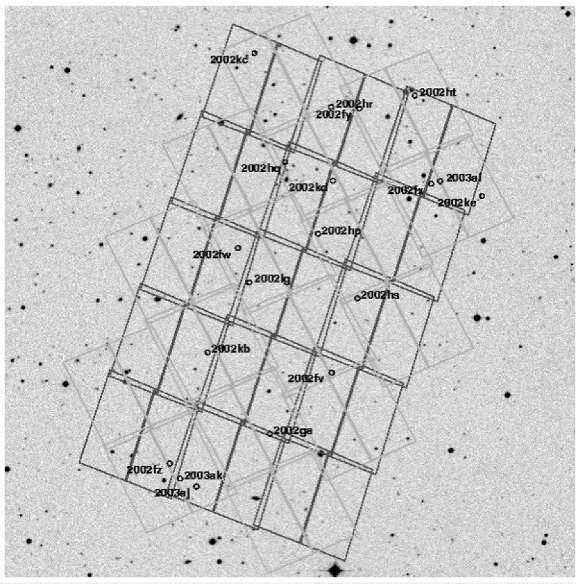
Figure 2: Same as in Figure 1, but for first (dark) and second (grey) epochs the CDFS field. Subsequent epochs are rotated by the same amounts as indicated in Figure 1.

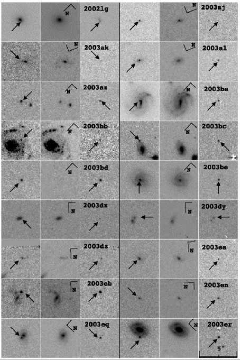
Figure 4: Same as in Figure 3, but for SN 2002lg through SN 2003er.

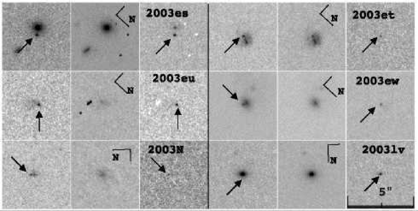
Figure 5: Same as Figure 3, but for SN 2003es through SN 2003lv.

Figure 6: The accuracy of the photometric redshifts as a function of actual spectroscopic redshift for the 26 SN host galaxies. Photometric redshifts were precise to $\sim 0.05$ RMS (rejecting two $>7\sigma$ outliers).

Figure 7: Flow chart showing how SN types and confidence ranks were determined from the data.

Figure 9: The efficiency of the survey in recovering false SNe in a pair of images (discovery and template) of a given difference magnitude. The histograms from both the real-time test (left), and from the Monte Carlo test (right) are shown. The Monte Carlo histogram is shown with Poisson errors (dark circles). The solid line shows the fit of the form $\epsilon(\Delta m)\propto(1+e^{\Delta m})^{-1}$ used to represent the efficiency. The dotted line (and open circles) show the maximum response to the psudo-Shaw Effect on the efficiency for this survey. For convenience, we roughly correlate the difference magnitude limits to redshift limits for SNe Ia discovered near maximum light, and to the optimum signal-to-noise limits for a point source in a residual frame.

Figure 10: Monte Carlo test efficiencies for populations which are either nearly coincident with, or well separated from, the nuclei of their host galaxies ($r<5$ and $r>5$ pixels, respectively). Neither distribution, specifically the nearly coincident sample, show detectable deviation from fits drawn from the real-time test (dotted line), or the Monte Carlo simulation of the entire sample (solid line).

Figure 11: The delay time distribution models for the $e$-folding (top), wide Gaussian (middle), and narrow Gaussian (bottom) functions. Each model is plotted with several values of $\tau$.

Figure 12: The probability distributions for the $e$-folding (top panels; shown with and without metallicity cutoff), wide Gaussian (middle panels), and narrow Gaussian (bottom panels) models shown as a function of $\tau$ for the M1 (left panels) and M2 (right panels) SFR histories. Note that none of the $e$-folding models shows a clear maximum likelihood value of $\tau$, and that the overall probability values are low for the $e$-folding and wide Gaussian models. Only in the narrow Gaussian models are there maximum likelihood values and overall high probabilities.

Figure 13: The fraction of Monte Carlo runs which produce likelihood values equal to or less than the likelihood of the data for each model. Models which could not often produce redshift distributions similar to the observed distribution had a low success fractions (less than $50-60$%) and were therefore rejected as improbable models for the data. The selected range in success fraction was consistent with the 95% confidence interval in likelihood for each model.

Figure 14: The predicted number distributions of SNe Ia for each model for selected values of $\tau$. The solid line is for the M1 SFR$(z)$ and the dash-dotted line is for the M2 model. The dotted line shows the control time (or survey efficiency, scaled) with redshift. The systematic effects on the control time are shown in the top left panel (black points).These predicted distributions are compared to the observed number distribution of SNe Ia from this survey. Most models cannot adequately reproduce the observed redshift distribution. Only for the narrow Gaussian model in the range of $\tau\approx 4$ Gyr does the predicted distribution appear similar to the observed distribution.

Figure 15: SN distributions, in linear and log space, for the maximum likelihood values of $\tau$ of each delay time function (solid lines). Shown are the $e$-folding $\Phi(t_{d})$ for $\tau=10$ [E(10)], the wide Gaussian for $\tau=4.0$ [G(4.0, 2.0)], and the narrow Gaussian for $\tau=4.0$ [G(4.0, 0.8)]. The dashed lines represent predicted distributions of SN Ia delay times from various models (Yungelson & Livio, 2000, reproduced from Figure 2). Shown are the predictions from double degenerate mergers (DD-Ch), edge-lit detonations from subgiant donors (SG-ELD), and normal accretion/detonations from subgiant donors (SG-Ch). There is some similarity to our best-fit models.

Table 1: HHZSS+GOODS Supernovae

SN	Nickname	U. T.	R. A. (2000)	Decl. (2000)	SN Type	Confidence	Redshift	Source	N (arcsec)	E (arcsec)
2002fv	Apollo	2002 Sep 19.6	03:32:22.73	-27:51:09.4	CC	bronze	$\cdots$	$\cdots$	$\cdots$	$\cdots$
2002fw	Aphrodite	2002 Sep 19.9	03:32:37.52	-27:46:46.6	Ia	gold	1.30	spectrum	0.21	-0.51
2002fx	Athena	2002 Sep 20.8	03:32:06.80	-27:44:34.4	Ia	silver	1.40	spectrum	-0.04	-0.09
2002fy	Hades	2002 Sep 20.9	03:32:18.12	-27:41:55.6	Ia	silver	0.88	phot-z	0.00	0.00
2002fz	Artemis	2002 Sep 21.6	03:32:48.54	-27:54:17.6	CC	silver	0.84	spectrum	-1.66	1.30
2002ga	Atlas	2002 Sep 22.5	03:32:32.62	-27:53:16.7	Ia	bronze	0.99	spectrum	-0.08	0.21
2002hp	Thoth	2002 Nov 01.5	03:32:24.79	-27:46:17.8	Ia	gold	1.30	spectrum	0.02	-0.01
2002hq	Re	2002 Nov 01.5	03:32:29.94	-27:43:47.2	CC	bronze	0.67	spectrum	-0.18	-0.91
2002hr	Isis	2002 Nov 01.6	03:32:22.57	-27:41:52.2	Ia	gold	0.53	spectrum	0.05	0.03
2002hs	Bast	2002 Nov 02.2	03:32:18.59	-27:48.33.7	CC	bronze	0.39	spectrum	2.50	-0.27
2002ht	Osiris	2002 Nov 02.5	03:32:09.32	-27:41:29.3	Ia	bronze	0.90	phot-z	0.48	0.34
2002kb	Denethor	2002 Dec 20.1	03:32:42.42	-27:50:25.4	CC	gold	0.58	spectrum	-0.20	-0.01
2002kc	Bilbo	2002 Dec 21.5	03:32:34.72	-27:39:58.3	Ia	gold	0.21	spectrum	-0.85	-0.28
2002kd	Frodo	2002 Dec 21.6	03:32:22.34	-27:44.26.9	Ia	gold	0.74	spectrum	-0.98	-3.13
2002ke	Smeagol	2002 Dec 21.9	03:31:58.77	-27:45:00.7	CC	bronze	0.58	spectrum	-0.26	1.15
2002kh	Balder	2003 Jan 04.3	12:36:16.78	+62:14:37.7	Ia	bronze	0.71	phot-z	0.30	-1.20
2002ki	Nanna	2003 Jan 04.6	12:37:28.37	+62:20:39.1	Ia	gold	1.14	spectrum	0.00	-0.10
2002kl	Agugux	2003 Feb 22.0	12:37:49.30	+62:14:06.1	CC	silver	0.41	spectrum	-0.45	0.15
2002lg	Prometheus	2002 Jul 04.2	03:32:35.77	-27:47:58.8	Ia	gold	0.66	spectrum	-0.10	0.13
2003aj	Inanna	2003 Feb 03.2	03:32:44.33	-27:55:06.4	Ia	bronze	1.31	spectrum	-0.08	-0.03
2003ak	Gilgamesh	2003 Feb 03.2	03:32:46.90	-27:54:49.4	Ia	gold	1.55	spectrum	-0.39	0.28
2003al	Enki	2003 Feb 05.7	03:32:05.39	-27:44:29.2	Ia	silver	0.91	phot-z	0.07	-0.03
2003az	Torngasak	2003 Feb 20.9	12:37:19.67	+62:18:37.5	Ia	gold	1.27	spectrum	-0.08	-0.06
2003ba	Sedna	2003 Feb 21.0	12:36:15.88	+62:12:37.7	CC	bronze	0.29	spectrum	0.09	-0.18
2003bb	Raven	2003 Feb 21.6	12:36:24.47	+62:08:35.3	CC	silver	0.95	spectrum	-1.31	0.40
2003bc	Michabo	2003 Feb 21.8	12:36:38.06	+62:09:53.3	CC	silver	0.51	spectrum	-0.55	-1.10
2003bd	Anguta	2003 Feb 22.0	12:37:25.06	+62:13:17.5	Ia	gold	0.67	spectrum	$\cdots$	$\cdots$
2003be	Qiqirn	2003 Feb 22.1	12:36:25.97	+62:06:55.6	Ia	gold	0.64	spectrum	0.00	-0.12
2003dx	Phidippides	2003 Apr 04.5	12:36:31.70	+62:08:48.7	CC	bronze	0.46	phot-z	0.10	0.15
2003dy	Borg	2003 Jan 02.8	12:37:09.14	+62:11:01.2	Ia	gold	1.37	spectrum	-0.35	0.25
2003dz	Ashe	2003 Apr 04.8	12:36:39.91	+62:07:52.7	CC	bronze	0.48	phot-z	0.00	-0.25
2003ea	Connors	2003 Apr 05.7	12:37:12.04	+62:12:38.3	CC	bronze	0.89	phot-z	0.15	0.00
2003eb	McEnroe	2003 Apr 05.7	12:37:15.18	+62:13:34.6	Ia	gold	0.92	spectrum	-0.75	0.50
2003en	Odin	2003 Jan 03.2	12:36:33.12	+62:13:48.1	Ia	bronze	0.54	phot-z	0.10	0.07
2003eq	Elvis	2003 May 24.7	12:37:48.34	+62:13:35.3	Ia	gold	0.85	spectrum	0.10	-0.42
2003er	Janice	2003 May 25.4	12:36:32.27	+62:07:35.2	CC	silver	0.63	phot-z	0.70	-0.70
2003es	Ramone	2003 May 25.5	12:36:55.39	+62:13:11.9	Ia	gold	0.97	spectrum	0.30	-0.49
2003et	Jimi	2003 May 25.7	12:35:55.87	+62:13:32.8	CC	silver	0.83	phot-z	0.14	-0.50
2003eu	Lennon	2003 May 25.7	12:36:05.90	+62:11:01.6	Ia	silver	0.76	phot-z	0.30	-0.70
2003ew	Jagger	2003 May 21.8	12:36:27.78	+62:11:25.1	CC	bronze	0.66	phot-z	-0.10	-0.21
2003N	Loki	2003 Apr 04.7	12:37:09.14	+62:11:01.2	CC	bronze	0.43	spectrum	0.20	0.00
2003lv	Vilas	2003 Apr 04.7	12:37:28.89	+62:11:28.7	Ia	silver	0.86	spectrum	0.00	0.00

Note. — Offsets are given from the center of the host galaxy to supernova.

Table 2: HST Photometry

SN	Filter	JD + 2,452,000	Magnitude
2002fv	$F850LP$	536.74	25.07 (0.06)
		580.32	25.72 (0.11)
		628.29	26.27 (0.18)
	$F775W$	536.74	25.34 (0.06)
	$F606W$	536.83	26.54 (0.06)
2002fy	$F850LP$	490.30	23.77 (0.02)
		538.20	25.23 (0.07)
		579.72	26.40 (0.20)
	$F775W$	490.32	24.37 (0.03)
		538.19	26.06 (0.12)
	$F606W$	490.30	26.15 (0.04)
		538.18	28.16 (0.25)
2002fz	$F850LP$	538.96	24.94 (0.06)
		578.71	26.30 (0.19)
	$F775W$	538.92	25.20 (0.05)
		578.45	26.73 (0.21)
2002ga	$F850LP$	488.72	25.90 (0.13)
		539.65	24.50 (0.04)
		578.95	26.18 (0.17)
		628.70	26.79 (0.29)
	$F775W$	488.70	27.50 (0.41)
		539.65	25.26 (0.06)
		628.70	28.90 (1.25)
	$F606W$	488.64	27.87 (0.20)
		539.65	26.42 (0.05)
		628.70	29.0 (0.53)
2002hq	$F850LP$	580.90	25.34 (0.08)
	$F775W$	579.50	26.43 (0.11)
2002hs	$F850LP$	580.52	25.27 (0.07)
	$F775W$	580.37	26.05 (0.12)
	$F606W$	580.32	26.77 (0.07)
2002ht	$F850LP$	581.00	25.64 (0.10)
		630.17	26.13 (0.16)
	$F775W$	580.95	26.33 (0.15)
2002kb	$F850LP$	488.72	24.62 (0.04)
		539.79	25.10 (0.06)
		578.95	25.60 (0.10)
	$F775W$	488.70	24.83 (0.04)
		539.78	25.17 (0.05)
		578.80	25.84 (0.09)
	$F606W$	488.65	25.02 (0.02)
		539.71	27.01 (0.06)
2002ke	$F850LP$	630.11	25.52 (0.09)
	$F775W$	630.03	26.00 (0.11)
	$F606W$	630.02	27.60 (0.15)
2002kh	$F850LP$	642.27	24.62 (0.04)
	$F775W$	642.27	25.64 (0.11)
	$F606W$	642.22	28.4 (0.8)
2002kl	$F850LP$	600.04	24.95 (0.08)
		642.66	25.42 (0.09)
	$F775W$	600.04	25.39 (0.06)
		642.66	26.32 (0.14)
	$F606W$	599.99	26.37 (0.05)
		642.57	27.81 (0.18)
2002lg	$F850LP$	464.83	24.31 (0.04)
		489.17	25.89 (0.13)
	$F775W$	489.19	26.80 (0.22)
2003aj	$F850LP$	666.3	25.60 (0.10)
		673.31	25.40 (0.10)
		688.3	26.50 (0.23)
	$F775W$	673.30	26.60 (0.19)
2003al	$F850LP$	676.02	24.59 (0.04)
	$F775W$	676.10	25.56 (0.08)
	$F606W$	675.89	28.95 (0.51)
2003ba	$F850LP$	691.24	23.63 (0.02)
	$F775W$	691.24	24.04 (0.02)
	$F606W$	691.16	25.03 (0.02)
2003bb	$F850LP$	692.11	25.59 (0.10)
	$F775W$	692.10	25.34 (0.06)
		732.84	26.17 (0.13)
	$F606W$	692.45	26.30 (0.05)
2003bc	$F850LP$	692.35	24.08 (0.03)
		733.84	24.66 (0.04)
		780.75	25.72 (0.11)
	$F775W$	692.12	24.10 (0.02)
		733.74	25.32 (0.06)
		781.06	25.96 (0.11)
	$F606W$	691.1	25.00 (0.02)
		733.84	27.33 (0.12)
		781.06	28.40 (0.31)
2003dx	$F850LP$	732.85	25.27 (0.07)
	$F775W$	732.84	25.76 (0.11)
	$F606W$	732.81	28.37 (0.31)
2003dz	$F850LP$	733.86	25.14 (0.07)
	$F775W$	733.86	25.39 (0.06)
	$F606W$	733.86	26.14 (0.04)
2003ea	$F850LP$	783.72	25.40 (0.09)
	$F775W$	783.66	26.00 (0.11)
	$F606W$	783.65	27.50 (0.14)
2003en	$F850LP$	642.31	25.60 (0.10)
	$F775W$	642.30	26.10 (0.20)
	$F606W$	642.28	27.30 (0.12)
2003er	$F850LP$	784.51	23.22 (0.02)
	$F775W$	784.44	23.11 (0.01)
	$F606W$	784.61	23.21 (0.01)
2003et	$F850LP$	784.94	25.38 (0.08)
	$F775W$	784.83	25.54 (0.07)
	$F606W$	784.92	25.90 (0.04)
2003eu	$F850LP$	784.94	24.40 (0.04)
	$F775W$	784.93	25.04 (0.05)
	$F606W$	784.92	26.79 (0.08)
2003ew	$F850LP$	646.86	24.21 (0.03)
		690.57	24.36 (0.04)
	$F775W$	646.85	24.83 (0.04)
		690.49	25.05 (0.05)
	$F606W$	646.85	26.92 (0.08)
		690.49	27.51 (0.14)
2003N	$F850LP$	642.21	26.21 (0.18)
	$F775W$	642.19	26.43 (0.16)
	$F606W$	642.23	27.11 (0.10)

Note. — Magnitudes are in the Vega-based system. Photometric errors are in parentheses.

Table 3: Likelihood Statistics

Statistic	SFR Model	$e$-folding	$e$-folding w/ MCO	$G(\tau,0.5\tau$)	$G(\tau,0.2\tau$)
Max. Likelihood $\tau$	M1	$9.8$	$9.8$	4.0	4.0
	M2	$9.8$	$8.2$	3.2	3.2
95% Interval $\tau$	M1	$>2.6$	$>2.8$	$>2.8$	$3.6-4.6$
	M2	$>2.2$	$>2.0$	$>2.0$	$2.4-3.8$

Note. — 95% interval for narrow Gaussian models are determined symmetrically about maximum likelihood value. All others are given for $\tau>95\%$ confidence interval. Values are given in Gyrs.

References

- Aguirre (1999) Aguirre, A. N. 1999, ApJ, 512, L19
- Aldering, Knop, & Nugent (2000) Aldering, G., Knop, R., & Nugent, P. 2000, AJ, 119, 2110
- Barris et al. (2004) Barris, B. J., et al. 2004, ApJ, 604, 571
- Bennett et al. (2003) Bennett, C. L., et al. 2003, ApJS, 148, 1
- Bertin & Arnouts (1996) Bertin, E., & Arnouts, S. 1996, A&AS, 117, 393
- Branch, Fisher, & Nugent (1993) Branch, D., Fisher, A., & Nugent, P. 1993, ApJ, 106, 2383
- Brandt et al. (2001) Brandt, W. N., et al. 2001, AJ, 122, 2810
- Cappellaro, Evans, & Turatto (1999) Cappellaro, E., Evans, R., & Turatto, M. 1999, A&A, 351, 459
- Dahlén & Fransson (1999) Dahlén, T., & Fransson, C. 1999, A&A, 350, 349
- Dahlen et al. (2004) Dahlen, T., et al. 2004, ApJ, submitted
- Duquennoy & Mayor (1991) Duquennoy, A., & Mayor, M. 1991, A&A, 248, 485
- Efstathiou et al. (2002) Efstathiou, G., et al. MNRAS, 330, L29
- Filippenko (1997) Filippenko, A. V. 1997, ARAA, 35, 309
- Gal-Yam et al. (2003) Gal-Yam, A., Maoz, D., Guhathakurta, P., & Filippenko, A. 2003, AJ, 125, 1087
- Gal-Yam & Maoz (2004) Gal-Yam, A., & Maoz, D. 2004, MNRAS, 347, 942
- Germany et al. (2004) Germany, L. M., et al., 2004, A&A, 415, 863
- Germany & Strolger (2004) Germany, L. M., & Strolger, L. -G., in preparation
- Giacconi et al. (2002) Giacconi, R., et al. 2002, ApJS, 139, 369
- Giavalisco et al. (2004a) Giavalisco, M., et al. 2004a, ApJ, 600, L93
- Giavalisco et al. (2004b) Giavalisco, M., et al. 2004b, ApJ, 600, L103
- Gilliland & Riess (2002) Gilliland, R. L., & Riess, A. 2002, in The 2002 HST Calibration Workshop: Hubble after the Installation of the ACS and the NICMOS Cooling System, ed. S. Arribas, A. Koekemoer, & B. Whitmore (Baltimore: Space Telescope Science Institute), 61
- Hachisu, Kato, & Nomoto (1996) Hachisu, I., Kato, M., & Nomoto, K. 1996, ApJ, 470, L97
- Hachisu et al. (1999) —. 1999, ApJ, 522, 487
- Hachisu & Kato (2003) Hachisu, I., & Kato, M. 2003, ApJ, 588, 1003
- Hamuy et al. (2000) Hamuy, M., Trager, S. C., Pinto, P. A., Phillips, M. M., Schommer, R. A., Ivanov, V., & Suntzeff, N. B. 2000, AJ, 120, 1479
- Hamuy & Pinto (2002) Hamuy, M., & Pinto, P. A. 2002, ApJ, 566, L63
- Hamuy et al. (2003) Hamuy, M., et al. 2003, Nature, 424, 651
- Han & Podsiadlowski (2003) Han, Z.-W., & Podsiadlowski, P. 2004, MNRAS, submitted
- Hardin et al. (2000) Hardin, D., et al. 2000, A&A, 362, 419
- Iben & Tutukov (1984) Iben, I., & Tutukov, A. V. 1984, ApJS, 54, 335
- Jha et al. (1999) Jha, S., et al. 1999, ApJS, 125, 73
- Kobayashi et al. (1998) Kobayashi, C., Tsujimoto, T., Nomoto, K., Hachisu, I., & Kato, M. 1998, ApJ, 503, L155
- Koekemoer et al. (2002) Koekemoer, A. M., Fruchter, A. S., Hook, R., & Hack, W. 2002, in The 2002 HST Calibration Workshop: Hubble after the Installation of the ACS and the NICMOS Cooling System, ed. S. Arribas, A. Koekemoer, & B. Whitmore (Baltimore: Space Telescope Science Institute), 337
- Li et al. (2001) Li, W., Filippenko, A. V., Treffers, R. R., Riess, A. G., Hu, J., & Qiu, Y. 2001, ApJ, 546, 734
- Lira (1995) Lira, P. 1995, Master’s thesis, Universidad de Chile
- Livio (1995) Livio, M. 1995, in ASP Conf. Ser. 72: Millisecond Pulsars. A Decade of Surprise, ed. A. Fruchter, M. Tavani, & D. Backer (San Francisco: ASP), 105
- Livio (2001) Livio, M. 2001, in Supernovae and Gamma-Ray Bursts: The Greatest Explosions since the Big Bang, ed. K. Sahu, M. Livio, N. Panagia (Cambridge: Cambridge University Press), 334
- Livio & Riess (2003) Livio, M., & Riess, A. G. 2003, ApJ, 594, L93
- Mack et al. (2003) Mack, J., et al. 2003, ACS Data Handbook, Version 5.0, Space Telescope Science Institute
- Madau, Della Valle, & Panagia (1998) Madau, P., Della Valle, M., & Panagia, N. 1998, MNRAS, 297, L17
- Madau, Pozzetti, & Dickinson (1998) Madau, P., Pozzetti, L., & Dickinson, M. 1998, ApJ, 498, 106
- Mobasher et al. (2004) Mobasher, B., et al.. 2004, ApJ, 600, L167
- Nomoto et al. (2000) Nomoto, K., Umeda, H., Kobayashi, C., Hachisu, I., Kato, M., & Tsujimoto, T. 2000, in Cosmic Explosions (AIP Conference Proceedings, 522), ed. S. Holt & W. Zhang (College Park: American Institute of Physics), 35
- Nugent, Kim, & Perlmutter (2002) Nugent, P., Kim, A., & Perlmutter, S. 2002, PASP, 114, 803
- Pain et al. (2002) Pain, R., et al., 2002, ApJ, 577, 120
- Panagia (2003) Panagia, N. 2003, in Lecture Notes in Physics, ed. K. W. Weiler (Heidelberg: Springer-Verlag), 113
- Peacock et al. (2001) Peacock, J. A., et al. 2001, Nature, 410, 169
- Percival et al. (2001) Percival, W. J., et al. 2001, MNRAS, 327, 1297
- Perlmutter et al. (1997) Perlmutter, S., et al. 1997, ApJ, 483, 565
- Perlmutter et al. (1999) Perlmutter, S., et al. 1999, ApJ, 517, 565
- Phillips (1993) Phillips, M. M. 1993, ApJ, 413, L105
- Phillips et al. (1999) Phillips, M. M., Lira, P., Suntzeff, N. B., Schommer, R. A., Hamuy, M., & Maza, J. 1999, AJ, 118, 1766
- Poznanski et al. (2002) Poznanski, D., Gal-Yam, A., Maoz, D., Filippenko, A. V., Leonard, D. C., & Matheson, T. 2002, PASP, 114, 833
- Richardson et al. (2002) Richardson, D., Branch, D., Casebeer, D., Millard, J., Thomas, R. C., & Baron, E. 2002, AJ, 123, 745
- Riess et al. (1996) Riess, A. G., Press, W. H., & Kirshner, R. P. 1996, ApJ, 473, 88
- Riess et al. (1998) Riess, A. G., et al.1998, AJ, 116, 1009
- Riess et al. (1999) Riess, A. G., et al. 1999, AJ, 118, 2675
- Riess et al. (2000) Riess, A. G., et al. 2000, ApJ, 536, 62
- Riess (2002) Riess, A. G. 2002, in The 2002 HST Calibration Workshop: Hubble after the Installation of the ACS and the NICMOS Cooling System, ed. S. Arribas, A. Koekemoer, & B. Whitmore (Baltimore: Space Telescope Science Institute), 47
- Riess et al. (2004a) Riess, A. G., et al. 2004a, ApJ, 600, L163
- Riess et al. (2004b) Riess, A. G., et al. 2004b, ApJ, in press
- Ruiz-Lapuente & Canal (1998) Ruiz-Lapuente, P., & Canal, R. 1998, ApJ, 497, L57
- Shaw (1979) Shaw, R. L. 1979, A&A, 76, 188
- Sirianni et al. (2003) Sirianni, M., et al. 2003, in Future EUV/UV and Visible Space Astrophysics Missions and Instrumentation, Proceedings of the SPIE, 4854J, ed. Blades & O. Siegmund, 496
- Strolger et al. (2002) Strolger, L. -G.,et al. 2002, AJ, 124, 2905
- Sullivan et al. (2003) Sullivan, M., et al. 2003, MNRAS, 340, 1057
- Tonry et al. (2003) Tonry, J. L., et al. 2003, ApJ, 594, 1