Theoretical expectations for magnetic field measurements in molecular cloud cores

Abstract

The currently most viable methods to estimate magnetic field strengths in molecular cloud cores are Zeeman measurements and the Chandrasekhar-Fermi (CF) method. The CF-method estimates magnetic field strengths from polarimetry and relies on equipartition between the turbulent kinetic and turbulent magnetic energy in the observed region. Thus, its application to objects not dominated by hydromagnetic turbulence is questionable. We calibrate the CF-method and Zeeman measurements against numerical models of self-gravitating molecular cloud cores. We find – in agreement with previous results – that the CF-method is on the average accurate up to a factor of $2$, while a single estimate can be off by a factor of $7$. The CF-method is surprisingly robust even when applied to regions not dominated by hydromagnetic turbulence and in the face of small-number statistics. Zeeman measurements can systematically overestimate the field strength in high-density regions, if the field is predominantly oriented along the line of sight, while they tend to underestimate the field in other cases.

1. Motivation

Magnetic fields are omnipresent in the interstellar medium (ISM). Their importance depends on their strength. The large-scale Galactic magnetic field contributes to the scale height of the Galactic disk, and it confines cosmic rays to the Galaxy, thus influencing the chemistry in molecular clouds. Molecular cloud cores – thought to be gravitationally unstable without an additional support mechanism – have been supposed to be stabilized by magnetic fields, leading to the model of magnetically mediated (low mass) star formation (Shu et al., 1987). An alternative – although not necessarily exclusively so (Lin & Nakamura, 2004) – model pictures magnetic fields as dynamically unimportant, and star formation being controlled mainly by turbulence on dynamical time scales (e.g. Larson 1981; Elmegreen 2000; Hartmann et al. 2001; Mac Low & Klessen 2004).

Magnetic field strength estimates in molecular cloud cores thus might provide a way to distinguish between those two models. Such measurements rely mostly on the Zeeman effect (e.g. Crutcher 1999, Bourke et al. 2001, Sarma et al. 2002) resulting in an estimate of the density-weighted, direction-sensitive integrated magnetic field strength along the line of sight, and on the Chandrasekhar-Fermi method (Chandrasekhar & Fermi, 1953). The CF-method relates the line of sight velocity dispersion to the plane of sky polarization angle dispersion under the assumption of an isotropically turbulent medium whose turbulent kinetic and turbulent magnetic energy components are in equipartition, yielding an estimate of the mean field

$$\langle B\rangle^{2}=4\pi\rho\frac{\sigma(v)^{2}}{\sigma(\theta)^{2}}.$$ (1)

In its original form as given by Chandrasekhar & Fermi (1953), equation (1) assumes small angles around the (required) mean field direction. Calibrations of the method with the help of numerical simulations of magnetized turbulent molecular cloud regions show that the CF-method on average overestimates the “true” field strength by a factor of approximately $2$ (Ostriker et al. 2001; Padoan et al. 2001; Heitsch et al. 2001b, in the following HZMLN). Limited observational resolution (mimicked by smoothing the simulated polarization maps with a Gaussian) leads to a further systematic overestimate (HZMLN). While the method is reasonably robust when selecting for small angles (Ostriker et al., 2001), it fails utterly for vanishing mean fields in the plane of sky, as expected (HZMLN). The latter authors suggested a modification of the CF-method which estimates not the mean field $\langle B\rangle$, but the rms field $\langle B^{2}\rangle^{1/2}$.

The CF-method complements Zeeman estimates to some extent, since it infers the mean field strength in the plane of sky. The hope is to actually retrieve information about the 3D structure of the magnetic field (Lai et al., 2003). Many of the more recent applications of the CF-method refer to the dense phases of the ISM, mostly to molecular cloud cores or Bok globules (e.g. Lai et al. 2001; Henning et al. 2001; Lai et al. 2002; Matthews et al. 2002; Lai et al. 2003, Wolf et al. 2003; Crutcher et al. 2004). Vallée et al. (2003) decided not to use the CF-method because of the uncertainty introduced by the line-of-sight averaging of the polarization pattern. Since the method relies on equipartition between the turbulent kinetic and magnetic energy, its application to other regimes than those dominated by hydromagnetic turbulence might raise some questions that we will discuss in §2.

The goal of this study is twofold: First we aim at establishing how reliable the CF-estimates are for regions which are not dominated by hydromagnetic turbulence. We calibrate the method with the help of cores in a high resolution model of self-gravitating magnetized turbulence (Li et al., 2004). We find that the CF-method returns on average reliable estimates (within a factor of $2$) as long as the full angle information is used. Single estimates can be off by a factor of $7$. The method is surprisingly robust even when it is applied to rotating and self-gravitating cores. Despite its robustness, the method is subject to various systematic effects.

Second, we use the model cores to infer Zeeman measurements of the field strengths and to compare those to the CF-estimates. While Zeeman measurements are expected to underestimate the magnetic field in a turbulent region because of cancellation along the line of sight, we find that they can systematically overestimate the field in high-density regions with ordered fields oriented parallel to the line of sight.

2. The CF-method in cores: systematic effects

The CF-method in its original form rests on four assumptions: (a) The field perturbations are caused by hydromagnetic turbulence. (b) The turbulent kinetic and turbulent magnetic energy are in equipartition (This is guaranteed for Alfvénic perturbations, see e.g. Zweibel & McKee (1995).). (c) The turbulence is isotropic. (d) The field is perfectly frozen to the (total) gas density. If one or more of these assumptions are violated, systematic effects will be introduced in the CF-estimates (see e.g. Zweibel (1990), Myers & Goodmann (1991), Zweibel (1996) and Crutcher et al. (2004) for a discussion). In the context of protostellar cores, two effects would be expected to play a major role:

(i) The field perturbations are caused by other agents than turbulence, namely self-gravitation and/or rotation. First, we could imagine a core within the picture of magnetically dominated star formation: The core is permeated by a strong field, rendering the system subcritical (e.g. Mouschovias & Spitzer (1976)). Turbulence is assumed to be negligible. The field would be expected to evolve to an hourglass-like structure, which the CF-method would in turn interpret as an effect of turbulence, thus underestimating the field strength.

Second, let us consider a flattened rotating core seen face on such, that the rotation axis is more or less parallel to the line of sight. The mean magnetic field vector is oriented parallel to the line of sight (This is the situation envisaged in the concept of magnetic braking of cores, see e.g. Lüst & Schlüter (1955); Mestel (1959)). The field lines would wind up, i.e. in projection they would describe spirals. These would result in large polarization angle dispersions not necessarily accompanied by a large velocity dispersion along the line of sight.

(ii) For anisotropic turbulence (see e.g. Cho & Lazarian (2003)), relating the line of sight velocity dispersion to the polarization angle dispersion can introduce a systematic effect in the CF-estimate. However, if the magnetic field is predominantly in the plane of sky, the CF-method could still yield reasonable results despite severe anisotropy.

3. Models and Methods

The model this study rests on is described in detail by Li et al. (2004). It mimics a fraction of an isothermal molecular cloud region (periodic boundary conditions), which is dominated by supersonic turbulence driven on the largest scales at Mach $10$ such that the driving energy input is kept constant (for a detailed description see Mac Low (1999)). Once an equilibrium state between driving energy input and dissipation has been reached, self-gravity is switched on. The shock-generated filaments start to fragment and form cores, the objects of this study. The initial ratio of thermal to magnetic pressure is $\beta=0.9$. For a detailed discussion of this type of simulation and the choice of parameters see e.g. Heitsch et al. (2001a).

Cores selected for this study have to fulfill several criteria: (a) They are gravitationally bound. (b) They are resolved according to the so-called Jeans-criterion (Truelove et al., 1997), given by

$$\lambda_{J}\equiv\sqrt{\frac{\pi}{G\rho}}c_{s}>4\Delta x,$$ (2)

where $\Delta x$ is the grid spacing and $c_{s}$ is the sound speed. (c) Regions of surface densities of $10$% of the peak surface density or above are used for analysis. Although this (excitation-) threshold is chosen somewhat arbitrarily (albeit guided by observational maps), other choices (within reasonable limits) did not affect the results. (d) Selected cores consist of more than $1000$ cells in order to sample their internal structure sufficiently. The sample cores are listed in Table 1. The fourth column in the table denotes unresolved cores according to the Jeans criterion. These cores are not used for the subsequent analysis except to demonstrate resolution effects. Note that $\rho/\rho_{J}$ gives a resolution criterion, while $M/M_{J}$ determines whether a core is gravitationally unstable. Here, $M_{J}$ is the thermal Jeans mass.

Table 1Properties of sample cores

core	$\rho/\rho_{J}$	# cells		$M/M_{J}$	$\cal{M}$	$\beta$	${\cal M}_{A}$	$t/\tau_{ff}$
d04c04	$0.32$	5956		$1.4$	$0.2$	$2.2$	$0.2$	$0.50$
d05c02	$0.33$	5283		$1.3$	$0.3$	$1.9$	$0.3$	$0.67$
d06c11	$0.28$	3589		$1.6$	$0.5$	$3.7$	$0.7$	$0.83$
d06c15	$0.22$	2928		$0.8$	$0.5$	$1.1$	$0.4$	$0.83$
d07c04	$5.68$	2167	X	$5.4$	$1.0$	$2.0$	$1.0$	$1.00$
d07c05	$2.44$	1194	X	$2.7$	$0.7$	$2.3$	$0.8$	$1.00$
d07c11	$0.55$	1574		$1.8$	$0.6$	$0.8$	$0.4$	$1.00$
d08c01	$70.6$	2043	X	$23$	$1.4$	$0.7$	$0.8$	$1.17$
d08c02	$57.6$	2056	X	$21$	$1.2$	$1.9$	$1.2$	$1.17$
d08c09	$9.58$	1133	X	$6.5$	$1.0$	$1.6$	$0.9$	$1.17$
d08c17	$0.26$	2344		$2.2$	$0.3$	$6.8$	$0.6$	$1.17$
d08c19	$0.26$	1354		$0.5$	$0.3$	$8.1$	$0.6$	$1.17$
d09c14	$0.91$	1440		$1.8$	$0.4$	$1.5$	$0.4$	$1.33$
d09c19	$0.35$	1130		$1.2$	$0.2$	$3.3$	$0.3$	$1.33$

Note. — First column: core label: dicj, where $i$ denotes the time dump number and $j$ specifies the core number at time dump $i$. Second column: maximum over Jeans density, derived from the stability criterion following Truelove et al. (1997). Unresolved cores are marked with an X in the fourth column. Third column: number of cells within core. Fifth column: mass contained in core over Jeans mass, assuming a spherical gas distribution. Sixth column: Mach number derived from (density-weighted) line-of-sight velocity dispersion. Seventh column: plasma beta $\beta=2\bar{\rho}c_{s}^{2}/B^{2}$. Eighth column: Alfvén Mach number ${\cal M}_{A}=v_{rms}/c_{A}$ where the Alfvén speed $c_{A}=B/\sqrt{4\pi\rho}$. Ninth column: dump time in units of the global free fall time $\tau_{ff}=\sqrt{3\pi/(32G\rho)}\approx 10^{6}$yrs.

Summarizing Table 1, the model cores are marginally gravitationally bound, their internal velocities are (in most cases) subsonic (${\cal M}\approx 0.5$), and the magnetic pressure is on the order of the thermal pressure (with a substantial scatter).

Once cores have been identified over the run of the simulation, we construct surface density maps and polarization maps following Zweibel (1996) via

$$P=Q+iU=N\int f(y)\frac{(B_{x}+iB_{z})^{2}}{B_{x}^{2}+B_{z}^{2}}\,\cos^{2}\gamma\,dy$$ (3)

where $B_{x}$ and $B_{z}$ give the field vectors in the plane of sky perpendicular to the line of sight and are taken directly from the simulations. We integrate along the line of sight in $y$-direction. The function $f(y)$ is a weighting function which accounts for the density, emissivity, and polarizing properties of the dust grains. As the simplest assumption, we take $f(y)$ to be the local gas density normalized by the column density $1/N=\int f(y)\,dy$, where we take the opportunity to correct a typo in HZMLN. The factor

$$\cos^{2}\gamma=\frac{B_{x}^{2}+B_{z}^{2}}{B_{x}^{2}+B_{y}^{2}+B_{z}^{2}}$$ (4)

accounts for suppression of polarization by the magnetic field component along the line-of-sight (e.g. Fiege & Pudritz (2000), Padoan et al. (2001)). The polarized intensity is $|P|=\sqrt{Q^{2}+U^{2}}$, and the polarization angle is

$$\phi=\frac{1}{2}\arctan{\frac{U}{Q}}.$$ (5)

Equation (3) is an approximate solution of the full radiative transfer equation for the Stokes parameters, (Martin 1974; Lee & Draine 1985), valid for small polarization and low optical depth. At far infrared wavelengths, and at typical column densities for molecular clouds, the medium can safely be assumed to be optically thin (Hildebrand et al., 2000). We deliberately leave out any statement about the polarization degree as we are only interested in the polarization angles, but not in the ratio between polarized and continuum intensity. By this we intend to keep the argument as simple as possible, not embarking on a discussion on the efficiency of grain alignment mechanisms (see e.g. Lazarian (2003)). This simplification certainly limits our study to the investigation of polarization angles only. To mimic limited telescope resolution, we smooth the polarization maps with a Gaussian filter as in HZMLN.

The CF-method is applied to the “polarization maps” in the extended form given by

$$\langle B\rangle^{2}=4\pi\rho\frac{\sigma(v)^{2}}{\sigma(\tan\theta)^{2}},$$ (6)

where we replace the small-angle approximation by the $\tan$ of the angle. The density is determined from the column densities of the polarization maps, assuming a spherical mass distribution, where the radius is given by the geometric mean of the long and short axis of the core (Crutcher et al., 2004).

To infer a “Zeeman” estimate from our cores, we integrate

$$\langle B_{ZM}\rangle=N\int f(y)B_{y}\,dy$$ (7)

along the line of sight. $N$ and $f(y)$ are the same as in equation (3).

4. Results

In order to establish the reliability of the CF-method for cores, we generated polarization maps after rotating the cores such that the line of sight is either parallel to the mean flux direction (the “worst case” for the CF-method, since then the necessary mean field component would be expected to vanish) or perpendicular to the mean flux direction (“best” case). An example of the three-dimensional core structure and the resulting polarization maps is given in Figures 1 and 2. The depicted core is a typical example in the sense that it combines very ordered with turbulent field structure.

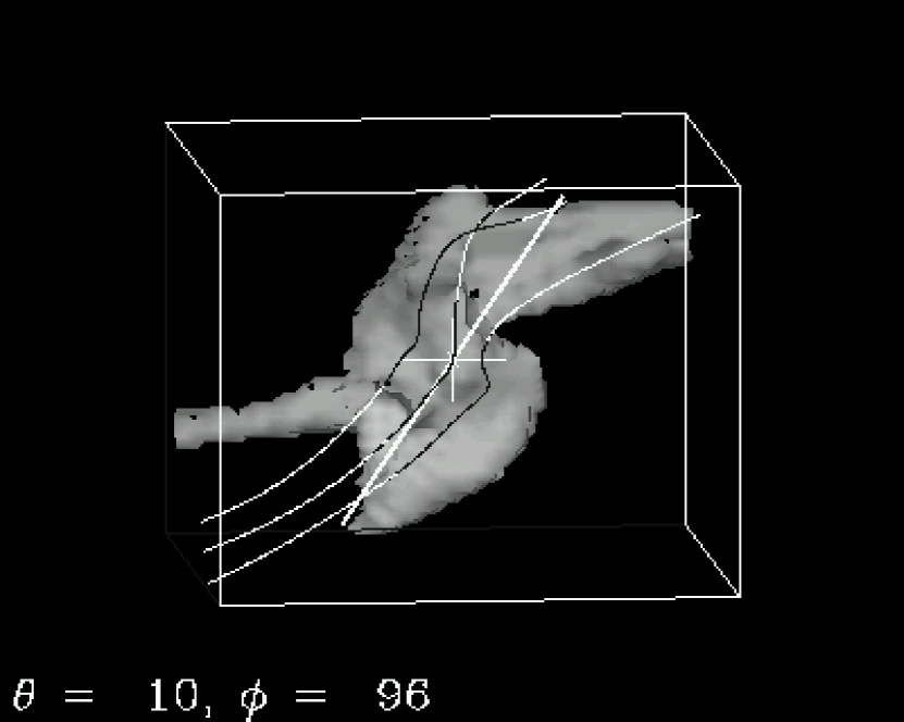
Figure 1.— 3D core projection. The core outline is given by iso-density surfaces. The straight line denotes the mean flux direction. Three representative field lines are outlined.

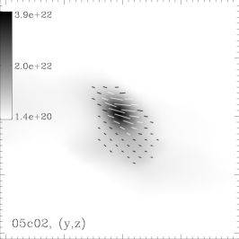
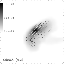
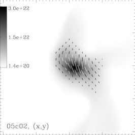
Figure 2.— (a) Polarization map looking along the mean flux direction. (b,c) Polarization map looking perpendicular to the mean flux direction denoted in Fig. 1. One panel measures approximately $0.25$pc across. The color bars give the column density in particles cm^-2. Every second polarization vector is shown (and used for the field estimate), resulting in a spatial “resolution” of $0.012$pc.

Figure 3 displays the three polarization maps – again seen along the mean flux direction and perpendicular to it – for the core shown in Figure 22 of Li et al. (2004). The oblate core is permeated by field lines oriented in parallel to its rotation axis. The field lines are slowly wound up, resulting in a spiral pattern when viewing the core along its rotation axis (left panel of Fig. 3). For the lines of sight perpendicular to the rotation axis, the rotation pattern does not emerge (center and right panel).

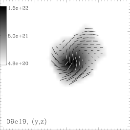
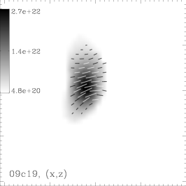
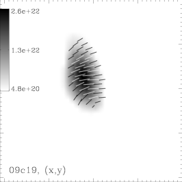
Figure 3.— (a) Polarization map looking along the mean flux direction for the core shown in Fig. 22 of Li et al. (2004). Note the spiral polarization pattern induced by the core’s rotation. (b,c) Polarization map looking perpendicular to the mean flux direction. One panel measures approximately $0.25$pc across. The color bars give the column density in particles cm^-2. Every second polarization vector is shown (and used for the field estimate), resulting in a spatial “resolution” of $0.012$pc.

4.1. Performance of the CF-method in cores

Figure 4 summarizes the reliability estimates for the CF-method applied to the resolved model cores (i.e. the ones without X’s in Table 1). For this plot, all three lines of sight were used. First, we note that using the small angle approximation (open symbols) leads to a systematic overestimate of the field strength by a factor of more than $4$. This is not surprising since we discard physically relevant information about the field structure (and thus strength) when selecting for small angles. However, we cannot restrict the line of sight velocity dispersion in the same way. On the other hand, using equation (6) (filled symbols) leads to a moderate overestimate of the field by a factor of approximately two. This is not inconsistent with the findings of Ostriker et al. (2001), since they selected for their whole domain and thus their results were not affected by small-number statistics. For large-number statistics, weak fields will lead to a wide angle dispersion, meaning that even when selecting, most of the angles are found at the largest possible values, thus indicating a weak field.

Figure 4.— Reliability $a=B_{CF}/\langle B\rangle$ versus the mean field in the core $\langle B\rangle$ for all resolved cores and lines of sight. Open symbols: angular dispersion selected for $\Delta\theta<25^{\circ}$. Filled symbols: angular dispersion selected for $\Delta\theta<85^{\circ}$. The dashed lines denote the averages, whose values are given in the plot. No smoothing applied. Clearly, selecting for $25^{\circ}$ leads to a systematic overestimate, while using the full information leads to an overestimate by approximately $2$ (lower dashed line).

Figure 5.— Reliability $a=B_{rms}/\langle B^{2}\rangle^{1/2}$ versus the rms mean field in the core $\langle B^{2}\rangle^{1/2}$ for all resolved cores and lines of sight. Open symbols: angular dispersion selected for $\Delta\theta<25^{\circ}$. Filled symbols: angular dispersion selected for $\Delta\theta<85^{\circ}$. The dashed lines denote the averages, whose values are given in the plot. No smoothing applied.

The small number of strong-field cores is conspicuous. This is simply a consequence of low initial field strength, which renders the turbulent box supercritical by a factor of $8$. On the one hand, this is inconsistent with the observations, on the other hand it allows us to test the CF-method under severer conditions than it would probably meet in observational data.

The modified method to estimate the rms field in the core gives – within the scatter – the same estimated field (Fig. 5). For smooth fields the method reverts to the original version, while for unordered fields, the method emphasizes the angular variations (see HZMLN for a discussion). The scatter of the estimates is slightly reduced. Note that on the whole the rms field is somewhat larger than the mean field, indicating a non-uniform field component in the cores.

Figures 4, 5 and all subsequent ones show cores extracted at different times during the simulation. Although we thus do not expect to be affected by selection effects that could result from chosing a special time instant during the simulation, there is of course a selection effect in the sense that we extract cores at comparable evolutionary stages, i.e. cores that are already self-gravitating, but still numerically resolved. As long as the cores are resolved, a correlation between reliability and global evolution time (last column in Table 1) cannot be seen.

Applying equation (6) and preventing the angular dispersion from blowing up by selecting for angle differences $\Delta\theta<85^{\circ}$ improves the reliability of the estimates in these models.

4.2. Effects of limited observational and numerical resolution

As HZMLN showed for extended regions, limited telescope resolution (finite beam width) leads to a systematic overestimate, because the field variations are averaged out, making the field look smoother, i.e. in terms of the method, stronger. We can observe a similar effect in Figure 6, compared to Figure 4. Degrading the resolution by roughly a factor of $3$ leads to an increased overestimate. The estimates selected for $\Delta\theta<25^{\circ}$ are less affected by the degraded resolution, and both selected sets of estimates agree for strong fields, as is to be expected.

It might be interesting to note that the ambipolar diffusion scale

$$L_{AD}=\frac{\lambda_{AD}}{v_{rms}}=1.97\times 10^{31}\frac{B^{2}}{x_{i}\,n_{n}^{2}\,v_{rms}}$$ (8)

is on the order of $0.01$pc for typical core parameters. In equation (8) the field strength $B$, the neutral particle density $n_{n}$ and the velocity dispersion $v_{rms}$ are given in cgs-units. The ionization fraction is denoted by $x_{i}$.

Figure 6.— Reliability $a=B_{CF}/\langle B\rangle$ versus the mean field in the core $\langle B\rangle$ for all resolved cores and lines of sight at reduced resolution (map smoothed with a Gaussian of $\sigma=3$pix). Open symbols: angular dispersion selected for $\Delta\theta<25^{\circ}$. Filled symbols: angular dispersion selected for $\Delta\theta<85^{\circ}$. The dashed lines denote the averages, whose values are given in the plot.

While Figure 6 demonstrated the effect of degraded telescope resolution, we exemplify the influence of under-resolved cores on the overall result in Figure 7.

Figure 7.— Reliability $a=B_{CF}/\langle B\rangle$ versus the mean field in the core $\langle B\rangle$ for all sample cores (including unresolved ones, see Tab. 1) and lines of sight. Open symbols: angular dispersion selected for $\Delta\theta<25^{\circ}$. Filled symbols: angular dispersion selected for $\Delta\theta<85^{\circ}$. The dashed lines denote the averages, whose values are given in the plot.

The effect is obvious: The peak densities in those cores start to grow unhampered once they overstep the resolution criterion. The peak is concentrated in the central cell, so that the field is not able to follow the density evolution (Heitsch et al., 2001a). Because of the over-large densities, the CF-method systematically overestimates the true field strength, a purely numerical effect in this case. Note that the overestimates correlate with the strongest fields and unresolved cores.

The insufficient numerical resolution leads to a diffusion of the field out of the dense region, qualitatively similar to ambipolar diffusion. While there is no basis on which to draw any conclusions from these under-resolved cores (especially since the numerical diffusion cannot be controlled, and can behave quite differently from its physical counterpart), a similar effect would be expected in the observations if the density tracer is a neutral species.

4.3. CF Method vs. Zeeman Effect

If the magnetic field is not uniform, Zeeman measurements – realized in our models via equation (7) – are expected to systematically underestimate the field strength because of cancellation by field reversals along the line of sight. At first glance, this expectation is not met (Fig. 8). The Zeeman-effect seems to overestimate the field roughly by the same amount as the CF-method does. However, distinguishing between the lines of sight clarifies the picture. Zeeman estimates taken along the mean flux direction – denoted by “los=1” in Figure 8 – yield larger values than those taken perpendicularly to the mean flux direction (“los=2” and “los=3”). Since the line of sight integration is density-weighted, fields at locations with higher densities tend to be emphasized. Because of flux-freezing, this generally means that there is a tendency to higher field strength estimates in cores with large density contrasts, leading to a systematic overestimate for such cores. Thus the estimates along the mean flux direction are dominated by the strongly weighted central field values, while the estimates perpendicular to the mean flux direction “see” the perturbed component around it, leading to cancellation. This of course holds only as long as the emissivity is (approximately) proportional to the density, as assumed in equation (7).

Figure 8.— Reliability for the Zeeman estimates $B_{ZM}/\langle B\rangle$ against the mean field in the core. Averages broken up according to line of sights are given in the plot, and los=1 means integration along the mean flux direction (as in Fig. 2).

Comparing the CF and Zeeman estimates in Figure 9, the picture is somewhat less clear for the CF-method. There is a slight tendency to a larger scatter for estimates along the mean flux direction (upper panel of Fig. 9, diamonds), as one would expect, since the method is expected to work most reliably for a strong mean field component in the plane of sky. Unfortunately, this is a reliability criterion gathered in “hindsight”, i.e. it is not possible to apply it to observational data.

Instead, we might be tempted to argue that for cases where the CF-method and the Zeeman measurements yield approximately the same results, the field value should be well determined. Filled symbols in Figure 9 denote estimates for which $B_{CF}$ and $B_{ZM}$ agree within a factor of three. The scatter is reduced for both the CF-method and the Zeeman-measurement, although we should note that the estimates could still be off by a factor of approximately five. It might be interesting to note that the overall scatter of the Zeeman measurements around the “true” field value is actually larger than that of the CF-estimates (Fig. 9).

Figure 9.— Reliability for the CF-estimates as in Figure 4 (upper panel) and for the “Zeeman” estimates $B_{ZM}/\langle B\rangle$ (lower panel) against the mean field in the core. The dashed line gives the mean reliability. los=1 means integration along the mean flux direction (as in Fig. 2). Filled symbols denote estimates for which $B_{CF}$ and $B_{ZM}$ agree within a factor of $3$, open symbols stand for the remaining estimates.

4.4. Effects on derived criticality of cores

Figure 10 demonstrates the scatter of the magnetic field estimates in terms of the criticality parameter $\lambda$ as defined by Crutcher et al. (2004), eq.(1), namely

$$\lambda=7.6\times 10^{-21}\frac{N(\mbox{H}_{2})}{B},$$ (9)

where the magnetic field $B$ is given in $\mu$G and the H₂ column density in cm^-2.

Figure 10.— Column density $N$ against magnetic field strength $B$ to estimate criticality of cores. The line gives $\lambda\equiv 1$ (see eq. [1] of Crutcher et al. (2004)). The symbols denote how $N(B)$ is determined. Diamonds: directly from simulations, squares: CF-Method, circles: Zeeman effect. Only resolved cores are shown (see Tab. 1), selected for $\Delta\theta<85^{\circ}$ in the case of the CF-estimates. Different symbols on constant lines of $N$ belong to one line of sight of one core. The star denotes $N(B)$ for the full simulation domain (i.e. $27$ pc³).

The tendency of the CF-method (squares in Fig. 10) to generally overestimate the field strength renders the core ensemble slightly more subcritical than expected from the numerical values (diamonds in Fig. 10). There are a few subcritical numerical data points (diamonds). These are strongly elongated filaments with fields aligned in parallel, indicating field line stretching. Although the numerical values already show a considerable scatter because of dynamical effects, the uncertainties in the CF-estimates as well as in the Zeeman-estimates emphasize that field estimates of single cores allow only a limited conclusion about the physical state of the core.

5. Discussion

Zeeman measurements and the CF-method are currently the most viable ways to estimate the magnetic field strength in the dense molecular medium. Since the two methods are measuring different components of the field, they complement each other to some extent. The CF-method rests on the assumption of equipartition between turbulent kinetic and turbulent magnetic energy in the medium, which is not necessarily guaranteed in regions dominated by e.g gravity or rotation, such as protostellar cores.

We tested with the help of model cores formed in a numerical simulation of self-gravitating magnetized turbulence how accurately the CF-method and Zeeman measurements can estimate the magnetic field strength in such cores. We find

1. that the CF-method is on the average surprisingly robust even in regions not dominated by turbulence. The previous overestimation factor of $2$ is still valid approximately for the model cores on the average, if the full angle dispersion information is used. Single measurements can be off by a factor of up to $7$ in both directions.

2. that applying the small-angle approximation in the CF-method leads to a systematic overestimate of $\langle B\rangle$.

3. that the “Zeeman” estimates of our cores can lead to an overestimate for integrations along the mean flux direction, resulting from the emphasis on strong fields from the density-weighted line of sight integration. For integrations perpendicular to the mean flux direction, the Zeeman measurements tend to underestimate the field strength. Thus, Zeeman measurements cannot generally be regarded as a lower limit on the field strength.

A major shortcoming of our model is its low field strength, which renders its regime less magnetized than observed in molecular cores. While this is definitely a limitation, we see it also as an advantage since the CF-method is expected to work more reliably for stronger field strengths (HZMLN). Obviously, further limitations of this study stem from the limited resolution within the cores.

Taking the emissivity proportional to the density (eq. 7) in the Zeeman estimates does not account for the fact that the tracer species do not necessarily contribute proportionally to gas density. In that sense, the overestimate inferred for the Zeeman measurements from our models could be regarded as an upper limit. We did not address the problem of how to convert tracer column densities into H₂ densities, which is very likely another major source of uncertainty in the CF-method. Similarly, we left out a discussion of the velocity tracers.

We conclude that single magnetic field estimates in molecular cores should be regarded with caution because of the substantial scatter. The CF-method works reliably on average and should be combined with other types of estimates.

References

- Bourke et al. (2001) Bourke, T. L., Myers, P. C., Robinson, G., & Hyland, A. R. 2001, ApJ, 554, 916
- Chandrasekhar & Fermi (1953) Chandrasekhar, S. & Fermi, E. 1953, ApJ, 118, 113
- Cho & Lazarian (2003) Cho, J. & Lazarian, A. 2003, MNRAS, 345, 325
- Crutcher (1999) Crutcher, R. M. 1999, ApJ, 520, 706
- Crutcher et al. (2004) Crutcher, R. M., Nutter, D. J., Ward-Thompson, D., Kirk, J. M. 2004, ApJ, 600, 279
- Elmegreen (2000) Elmegreen, B. G. 2000, ApJ, 530, 277
- Fiege & Pudritz (2000) Fiege, J. D. & Pudritz, R. E. 2000, ApJ, 544, 830
- Galli & Shu (1993) Galli, D. & Shu, F.H. 1993, ApJ, 417, 243
- Hartmann et al. (2001) Hartmann, L., Ballesteros-Paredes, J., Bergin, E. A. 2001, ApJ, 562, 852
- Heitsch et al. (2001a) Heitsch, F., Mac Low, M.-M., Klessen, R. S. 2001, ApJ, 547, 280
- Heitsch et al. (2001b) Heitsch, F., Zweibel, E. G., Mac Low, M.-M., Li, P. S., Norman, M. L. 2001, ApJ, 561, 800
- Henning et al. (2001) Henning, T., Wolf, S., Launhardt, R., Waters, R. 2001, ApJ, 561, 871
- Hildebrand et al. (2000) Hildebrand, R.H., Davidson, J.A., Dotson, J.L., Dowell, C.D., Novak, G., Vaillancourt, J.E. 2000, PASP, 112, 1215
- Lai et al. (2001) Lai, S.-P., Crutcher, R. M., Girart, J. M., Rao, R. 2001, ApJ, 561, 864
- Lai et al. (2002) Lai, S.-P., Crutcher, R. M., Girart, J. M., Rao, R. 2002, ApJ, 566, 925
- Lai et al. (2003) Lai, S., Girart, J. M., & Crutcher, R. M. 2003, ApJ, 598, 392
- Larson (1981) Larson, R. 1981, MNRAS, 194, 809
- Lazarian (2003) Lazarian, A. 2003, Journal of Quantitative Spectroscopy and Radiative Transfer, 79, 881
- Lee & Draine (1985) Lee, H.M. & Draine, B. T. 1985, ApJ, 290, 211
- Li et al. (2004) Li, P. S., Norman, M. L., Mac Low, M.-M., Heitsch, F. 2004, ApJ, 605, 800
- Lin & Nakamura (2004) Lin, Z.-F. & Nakamura, F. 2004, ApJ, 609, L83
- Lüst & Schlüter (1955) Lüst, R. & Schlüter, A. 1955, Zeitschrift für Astrophysik, 38, 190
- Mac Low (1999) Mac Low, M.-M. 1999, ApJ, 524, 169
- Mac Low & Klessen (2004) Mac Low, M.-M. & Klessen, R.S. 2004, \rmp, 76, 125
- Martin (1974) Martin, P.G. 1974, ApJ, 187, 461
- Matthews et al. (2002) Matthews, B. C., Fiege, J. D., Moriarty-Schieven, G. 2002, ApJ, 569, 304
- Mestel (1959) Mestel, L. 1959, MNRAS, 119, 249
- Mouschovias & Spitzer (1976) Mouschovias, T. C. & Spitzer, L. 1976, ApJ, 210, 326
- Myers & Goodman (1991) Myers, P. C. & Goodman, A. A. 1991, ApJ, 373, 509
- Ostriker et al. (2001) Ostriker, E.C., Stone, J.M., Gammie, C.F. 2001, ApJ, 546, 980
- Padoan et al. (2001) Padoan, P., Goodman, A., Draine, B. Juvela, M. Nordlund, Å., Rögnvaldsson, Ö. 2001, ApJ, 559, 1005
- Sarma et al. (2002) Sarma, A.P., Troland, T.H., Crutcher, R.M. & Roberts, D.A. 2002, ApJ, 580, 928
- Shu et al. (1987) Shu, F., Adams, F., Lizano, S. 1987, ARA&A, 25, 23
- Troland & Heiles (1986) Troland, T. H. & Heiles, C. 1986, ApJ, 339, 345
- Truelove et al. (1997) Truelove, J. K., Klein, R. I., McKee, C. F. et al. 1997, ApJ, 489, L179
- Vallée et al. (2003) Vallée, J. P., Greaves, J. S., Fiege, J. D. 2003, ApJ, 588, 910
- Wolf et al. (2003) Wolf, S., Launhardt, R., Henning, T. 2003, ApJ, 592, 233
- Zweibel (1990) Zweibel, E. G. 1990, ApJ, 362, 545
- Zweibel & McKee (1995) Zweibel, E. G. & McKee, C. F. 1995, ApJ, 439, 779
- Zweibel (1996) Zweibel, E. G. 1996, Polarimetry of the interstellar medium. ASP Conf. Ser.; vol. 97; San Francisco: ASP; —c1996; edited by Wayne G. Roberge and Doug C. B. Whittet, p.486