Pulsational Analysis of the Cores of Massive Stars and its Relevance to Pulsar Kicks

Abstract

The mechanism responsible for the natal kicks of neutron stars continues to be a challenging problem. Indeed, many mechanisms have been suggested, and one hydrodynamic mechanism may require large initial asymmetries in the cores of supernova progenitor stars. Goldreich, Lai, & Sahrling (1997) suggested that unstable g-modes trapped in the iron (Fe) core by the convective burning layers and excited by the $\epsilon$-mechanism may provide the requisite asymmetries. We perform a modal analysis of the last minutes before collapse of published core structures and derive eigenfrequencies and eigenfunctions, including the nonadiabatic effects of growth by nuclear burning and decay by both neutrino and acoustic losses. In general, we find two types of g-modes: inner-core g-modes, which are stabilized by neutrino losses and outer-core g-modes which are trapped near the burning shells and can be unstable. Without exception, we find at least one unstable g-mode for each progenitor in the entire mass range we consider, 11 M_☉ to 40 M_☉. More importantly, we find that the timescales for growth and decay are an order of magnitude or more longer than the time until the commencement of core collapse. We conclude that the $\epsilon$-mechanism may not have enough time to significantly amplify core g-modes prior to collapse.

1 Introduction

Observations indicate that many pulsars have high proper motions (Lyne & Lorimer 1994; Lorimer, Bailes, & Harrison 1997; Hansen & Phinney 1997; Cordes & Chernoff 1998) and that many neutron star systems require kicks at birth. For example, pulsar bow shock morphologies (Cordes, Romani, & Lundgren 1993), misaligned spins of binary pulsars (Cordes, Wasserman, & Blaskiewicz 1990; Kramer 1998; Wex, Kalogera, & Kramer 2000; Kaspi et al. 1996; Lai, Bildsten, & Kaspi 1995; Lai 1996; Kumar & Quataert 1997), the statistics of low-mass X-ray binaries (LMXBs) (Kalogera 1997; Kalogera & Webbink 1998), the high orbital eccentricities of some Be star systems (Verbunt & van den Heuvel 1995), and scenarios for double neutron star systems (Dewey & Cordes 1987; Fryer & Kalogera 1997; Fryer, Burrows, & Benz 1998; Dewi & van den Heuvel 2004; Willems & Kalogera 2004) all indicate that neutron stars experience significant natal kicks. Furthermore, Arzoumanian, Chernoff, & Cordes (2002) find a bimodal distribution of birth kick speeds with peaks at $\sim$100 km s^-1 and $\sim$700 km s^-1 and dispersions of 90 and 500 km s^-1. They suggest that roughly 50% of the pulsars in the solar neigborhood escape the Galaxy and that $\sim$15% have kick speeds greater than 1000 km s^-1. The observations indicate that kicks seem to be hallmarks of neutron star formation.

What is the mechanism producing the observed and inferred kicks? To give a $1.4$ M_☉ neutron star a speed of 1000 km s^-1, the mechanism must be able to impart $\sim$10⁴⁹ erg of kinetic energy, which is just 1% of the canonical SN mechanical energy ($\sim$10⁵¹ erg) or 0.01% of the collapse energy ($\sim$10⁵³ erg). Additionally, any explanation must address the distribution of speeds. If the distribution is bimodal, then it is possible that more than one mechanism is responsible for the kicks. Lai (2000b) has summarized the possible magnetic, neutrino ($\nu$), and hydrodynamic kick mechanisms, but in general many of the scenarios have trouble producing kicks larger than $\sim$200 km s^-1.

Of the many mechanisms propounded, hydrodynamic mechanisms are the most compelling. For example, neutrino-driven convection, which is inherently a nonspherical phenomenon, excites large-scale convective motions that stochastically jostle the protoneutron star (Burrows, Hayes, & Fryxell 1995; Janka & Müller 1994). However, multi-dimensional calculations indicate that any kick imparted as a result of the convective jostling (“Brownian motion”) has an average magnitude of $\sim$200 km s^-1 (Burrows et al. 1995; Janka & Müller 1994; Scheck et al. 2004) and cannot explain the highest velocities nor the second peak in a possible bimodal distribution.

These analyses suggest the need for additional asymmetries before the onset of collapse. Burrows & Hayes (1996) state that global asymmetries in the progenitor may be prerequisites for large kicks. In a 2-D hydrodynamic simulation and with modest asymmetries, Burrows & Hayes (1996) are able to produce a recoil speed of $\sim$550 km s^-1. However, these calculations are crude and the results, while suggestive, are not conclusive. Goldreich et al. (1997) have proposed that these asymmetries may be excited by the $\epsilon$-mechanism in which g-mode oscillations in the core are pumped by nuclear reactions.

As a prelude to more definitive multi-dimensional radiation hydrodynamic investigations of neutron star kicks in the supernova context, one would like to determine whether global asymmetries prior to core collapse in fact occur. Hence, a thorough analysis of the progenitor oscillations and their growth rates is necessary. In this paper, we explore the viability of the g-mode oscillation origin for putative pre-collapse anisotropies by performing such an eigenmode analysis.

2 Linear Perturbation Equations

To set the stage for our eigenmode analysis of the cores of nonrotating massive stars, we first describe linear stellar pulsation theory in the general case. In linear perturbation theory, a star is assumed to be in hydrostatic equilibrium, around which perturbations are small, making second-order or higher terms in the perturbation equations negligibly small. Therefore, if $f_{0}(\vec{r})$ is a quantity satisfying the hydrostatic equations, then $f(\vec{r},t)\rightarrow f_{0}(r)+f^{\prime}(\vec{r},t)$, where $0$ denotes the background solution and ^′ denotes the Eulerian perturbation. We assume that the perturbation is of the form $f^{\prime}(\vec{r},t)=f^{\prime}(r)Y_{lm}(\theta,\phi)e^{i\omega t}$, where $Y_{\ell m}(\theta,\phi)$ is a spherical harmonic in that $\ell$ and $m$ are the polar and azimuthal indeces, repsectively, and $\omega$ is the oscillation frequency. Under these assumptions and an assumption of adiabatic perturbations, if $P$, $\rho$, $\phi$, $c_{s}$ are the pressure, density, gravitational potential, and sound speed, respectively, the adiabatic linear peturbation equations are

$$\frac{1}{r^{2}}\frac{d}{dr}(r^{2}\xi_{r})-\frac{g}{c^{2}_{s}}\xi_{r}+\left(1-\frac{L^{2}_{l}}{\omega^{2}}\right)\frac{P^{\prime}}{\rho c_{s}^{2}}=\frac{l(l+1)}{\omega^{2}r^{2}}\phi^{\prime},$$ (1)

$$\frac{1}{\rho}\frac{dp^{\prime}}{dr}+\frac{g}{\rho c^{2}_{s}}P^{\prime}+(N^{2}-\omega^{2})\xi_{r}=-\frac{d\phi^{\prime}}{dr},$$ (2)

and

$$\frac{1}{r^{2}}\frac{d}{dr}\left(r^{2}\frac{d\phi^{\prime}}{dr}\right)-\frac{l(l+1)}{r^{2}}\phi^{\prime}=4\pi G\rho\left(\frac{P^{\prime}}{\rho c^{2}_{s}}+\frac{N^{2}}{g}\xi_{r}\right).$$ (3)

$\xi_{r}$ and $\xi_{h}$ are the radial and horizontal components of the Lagrangian displacement vector, $\vec{\xi}=\vec{r}-\vec{r_{0}}$, and are defined by

$$\vec{\xi}=\left(\xi_{r},\xi_{h}\frac{\partial}{\partial\theta},\xi_{h}\frac{\partial}{\sin{\theta}\partial\phi}\right)Y_{lm}(\theta,\phi)e^{i\omega t}$$ (4)

and

$$\xi_{h}=\frac{1}{\omega^{2}r}\left(\frac{P^{\prime}}{\rho}+\phi^{\prime}\right).$$ (5)

$N$ and $L_{\ell}$ are the Brunt-Väisälä and Lamb frequencies, respectively, which are given by

$$N^{2}=g\left(\frac{1}{\Gamma_{1}}\frac{dlnP}{dr}-\frac{dln\rho}{dr}\right)$$ (6)

and

$$L^{2}_{\ell}=\frac{\ell(\ell+1)c_{s}^{2}}{r^{2}},$$ (7)

where $g=GM_{r}/r^{2}$, $G$ is the gravitational constant, and $M_{r}$ is the mass interior to $r$.

Equations (1), (2), and (3) represent a fourth-order boundary value problem. Near $r\sim 0$, simplifications and regularity in the variables $\phi^{\prime}$, $\xi_{r}$, and $(P^{\prime}/\rho+\phi^{\prime})$ dictate that the inner boundary conditions are

$$\frac{d\phi^{\prime}}{dr}-\frac{\ell\phi^{\prime}}{r}=0$$ (8)

and

$$\xi_{r}-\ell\xi_{h}=0.$$ (9)

At the surface of the calculational domain, $r=R$ or $M_{r}=M$, one outer boundary condition, from the regularity of $\phi^{\prime}$, is

$$\frac{d\phi^{\prime}}{dr}+\frac{(l+1)}{r}\phi^{\prime}=0.$$ (10)

A second outer boundary condition allows for the possibility that the atmosphere is either evanescent to both p- and g-waves or progressive to outgoing p-waves (Lai 2000b), depending upon the mode frequency:

$$\left(\frac{\lambda_{-}-(V/\Gamma_{1}-3)}{b_{1}}\right)\frac{\xi_{r}}{r}-\frac{\omega^{2}}{g}\xi_{h}-\left(\frac{\alpha_{1}(\lambda_{-}-(V/\Gamma_{1}-3))}{b_{1}}-\alpha_{2}\right)\frac{\phi^{\prime}}{gr}=0,$$ (11)

where

$$\lambda_{-}=\text@frac{1}{2}\left(\frac{V}{\Gamma_{1}}+\frac{rN^{2}}{g}-2-\gamma^{1/2}\right),$$ (12)

$$\gamma=\left(\frac{rN^{2}}{g}-\frac{V}{\Gamma_{1}}+4\right)^{2}+4\left(\ell(\ell+1)\frac{GM}{\omega^{2}R^{3}}-\frac{V}{\Gamma_{1}}\right)\left(\frac{\omega^{2}R^{3}}{GM}-\frac{rN^{2}}{g}\right),$$ (13)

$$b_{1}=\frac{\ell(\ell+1)\omega^{2}R^{3}}{GM}-\frac{V}{\Gamma_{1}},$$ (14)

$$b_{2}=\frac{\omega^{2}R^{3}}{GM}-\frac{rN^{2}}{g},$$ (15)

$$\alpha_{1}=\frac{b_{1}(rN^{2}/g)-((1+rN^{2}/g)+\ell)V/\Gamma_{1}}{(V/\Gamma_{1}-3+\ell)(1+rN^{2}/g+\ell)-b_{1}b_{2}},$$ (16)

and

$$\alpha_{2}=\frac{b_{2}V/\Gamma_{1}-(V/\Gamma_{1}-3+\ell)rN^{2}/g}{(V/\Gamma_{1}-3+\ell)(1+rN^{2}/g+\ell)-b_{1}b_{2}}.$$ (17)

If the mode frequency is such that this boundary condition represents leakage of mode energy by progressive p-waves then the eigensolutions are complex, with the imaginary part of $\omega$, $\omega_{I}$, being related to the rate of leakage.

The solutions to the boundary and eigenvalue problem as defined by eqs. (1)-(3) with the boundary conditions, eqs. (8)-(11), are the eigenmodes of the perturbed star. The eigenvalue, $\omega^{2}$, and eigensolution depend on the stellar structure and spherical harmonic index, $\ell$, but without rotation are degenerate for different values of $m$. We have found solutions to this boundary value problem using a shooting technique, in which we search for all modes within a region of the complex plane of $\omega^{2}$. This is accomplished with a 2-D Newton-Raphson technique, where convergence to one part in $10^{6}$, or better, in the eigenvalue is required. We compare our eigensolutions and eigenfrequencies for the standard Solar model (Christensen-Dalsgaard et al. 1996) with the eigenmodes determined by a publicly accessible Fortran code designed to solve the adiabatic linear perturbation equations. The agreement between the two is better than 0.1%.

2.1 Work Integral

In general, non-adiabatic effects such as nuclear burning and neutrino emission are included in the perturbation equations. However, if these terms are small, the contributions to the imaginary part of $\omega$, $\omega_{I}$, which is directly related to the rate of growth or decay of the mode, can be obtained from the time-averaged work integral, $W_{j}$ (Unno et al. 1989). For a quasi-adiabatic oscillation,

$$W_{j}=\frac{\pi}{\omega}\int_{0}^{M}\epsilon_{j}\left(\epsilon_{jT}+\frac{\epsilon_{j\rho}}{\Gamma_{3}-1}\right)\left|\frac{\delta T}{T}Y_{lm}(\theta,\phi)\right|^{2}dM_{r},$$ (18)

where $\epsilon_{j}$ (erg g^-1 s^-1) is the deposition or loss of energy by either nuclear heating if $j=nuc$ or neutrino losses if $j=\nu$. Furthermore, $\epsilon_{jT}=(\partial ln\epsilon_{j}/\partial lnT)_{\rho}$, $\epsilon_{j\rho}=(\partial ln\epsilon_{j}/\partial ln\rho)_{T}$, and $\Gamma_{3}-1\equiv(\partial lnT/\partial\rho)_{S}$, where $S$ is the entropy. The radial distribution of the Lagrangian perturbation in temperature is given by

$$\frac{\delta T}{T}=V\nabla_{ad}\left(\frac{\omega^{2}}{g}\xi_{h}-\frac{\phi^{\prime}}{gr}-\frac{\xi_{r}}{r}\right),$$ (19)

where $\nabla_{ad}=(\partial lnT/\partial ln\rho)_{s}$ and $V=gr\rho/P$.

When $\omega$ is complex, as is the case when the mode gains or loses energy, the time dependence of the modes may be written as

$$\vec{\xi}\propto e^{i\omega_{R}t}e^{t/\tau},$$ (20)

where $\omega_{R}$ is the real part of $\omega$, and $\tau$ is the timescale for growth (+) or decay (-) and is a composite effect determined by the equation

$$\frac{1}{\tau}=\frac{1}{\tau_{nuc}}+\frac{1}{\tau_{\nu}}+\frac{1}{\tau_{leak}}.$$ (21)

$\tau_{nuc}$, $\tau_{\nu}$, and $\tau_{leak}$ include the effects of nuclear gains, neutrino losses, and acoustic losses, respectively. The nuclear and neutrino timescales are related to their respective work integrals by

$$\tau_{j}=\frac{4\pi E_{W}}{\omega_{R}W_{j}},$$ (22)

where $E_{W}$ is the energy in the mode:

$$E_{W}=\frac{\omega_{R}^{2}}{2}\int^{M}_{0}\left|\vec{\xi}\right|^{2}dM_{r},$$ (23)

and $\tau_{leak}$ is directly determined by the imaginary part of $\omega$, $Im(\omega)=-1/\tau_{leak}$. This quantity is the solution to the adiabatic linear perturbation equations when eq. (11) is the fourth boundary condition. The modes are stable or unstable for $\tau<0$ or $\tau>0$, respectively.

3 Massive Star Structures

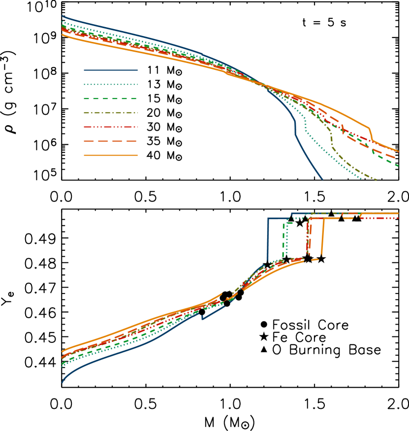
Figure 1: Density (top panel) and electron fraction, $Y_{e}$, (bottom panel) versuses interior mass, $M$, for the 11 M_☉ (solid and dark blue), 13M_☉ (dotted and light blue), 15 M_☉ (dashed and green), 20 M_☉ (dot-dash and olive green), 30 M_☉ (dot-dot-dot-dash and red), 35 M_☉ (long dashed and orange), and 40 M_☉ (solid orange) models, all at 5 s before the onset of collapse. Note in the top panel that the lower mass models have higher central densities, but that the higher mass models have shallower density gradients. Included on the $Y_{e}$ plot are points indicating significant features in the star, which greatly affect the modes. Circles represent the farthest extent of the fossil Fe core, which was formed during convective core Si burning. Stars represent the base of the Si burning shell at 5 seconds before the start of collapse (i.e., the extent of the Fe core, including the fossil Fe and the most recent ashes from Si shell burning), which generally aren’t convective until collapse. The triangles represent the base of the convective O burning shell

To investigate the character of the eigenmodes as a function of progenitor mass and time, $t$, prior to the onset of collapse, we consider the cores of nonrotating, massive stars with masses of 11 M_☉, 13 M_☉, 15 M_☉, 25 M_☉, 30 M_☉, 35 M_☉ and 40 M_☉ (Rauscher et al. 2002; Woosley, Heger, & Weaver 2002) and at $t=$ 3600, 600, 60, 30, 25, 20, 15, 10, 5, 2, 1, and 0 (start of collapse) seconds before the onset of collapse. The commencement of collapse is defined at the time when the peak infall velocity exceeds 900 km s^-1. This is about 200 to 250 ms before core bounce. The structure of each stellar model uniquely determines its eigenmodes. Thus, an indentification of important trends in the models is helpful in characterizing these modes. In the top panel of Fig. 1 we see that more massive models have higher entropy, translating into lower central densities and more extended density ($\rho$) versus interior mass, $M_{r}$, profiles. Consequently, prominent boundaries which are associated with discontinuities in entropy and $Y_{e}$ and which affect the character of the modes are also located at larger radii for higher-mass progenitors. These discontinuities are the boundary between the fossil Fe core (the residue of core Si burning) and the most recent Fe ashes from shell Si burning (circles on Fig. 1), the edge of the Fe core (includes the fossil Fe core and recent Fe ashes) and the Si burning shell (stars on Fig. 1), and the interface between the Si burning and O burning shells (triangles on Fig. 1). The general structural profiles and these distinct boundaries (Table 1) together determine the eigenfunctions and eigenfrequencies.

The role of structure in affecting the general character of the solutions can be understood using the local dispersion relation for plane waves of the form $e^{i(\vec{k}\cdot\vec{r}\pm\omega t)}$:

$$k^{2}_{r}=\frac{(N^{2}-\omega^{2})(L^{2}_{\ell}-\omega^{2})}{c_{s}^{2}\omega^{2}},$$ (24)

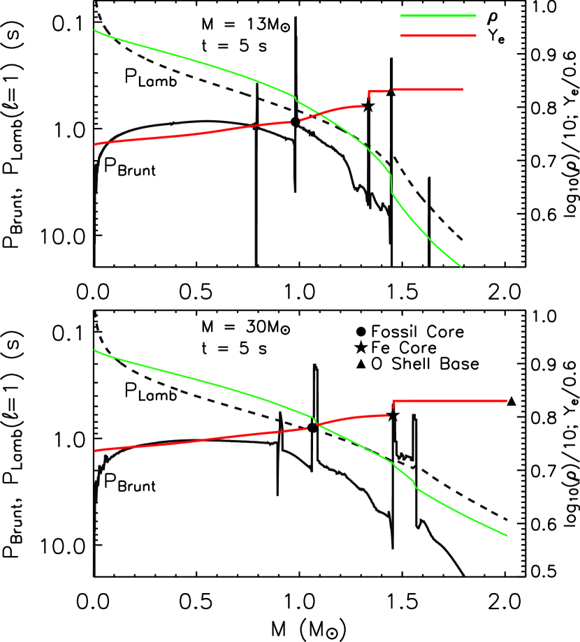
Figure 2: Density (solid green) and $Y_{e}$ (solid red) versuses interior mass in comparison to the propagation diagram for the 13 M_☉ model at 5 s before the onset of collapse. Usually, the square of the Brunt-Väisälä ($N^{2}$) and Lamb ($L^{2}_{\ell}$) frequencies are plotted. In this case, an equivalent period of oscillation is displayed instead, defined by $P_{Brunt}=2\pi/\sqrt{(}|N^{2}|)$ and $P_{Lamb}=2\pi/\sqrt{(}|L^{2}_{\ell}|)$. The circles, stars, and triangles represent the same structural boundaries as in Fig. 1. The vertical spikes are from discontinuous density and $Y_{e}$ changes in the profiles and are real. The bottom panel provides the equivalent information for the 30 M_☉ model.

where $k_{r}$ is the radial component of the wave vector (Unno et al. 1989). This relation implies that for $N^{2}<\omega^{2}<L^{2}_{\ell}$, all waves are evanescent, for $N^{2}<L^{2}_{\ell}<\omega^{2}$, they are p-waves, and for $\omega^{2}<N^{2}<L^{2}_{\ell}$, they are g-waves (Unno et al. 1989). A propagation diagram, which plots $N^{2}$ and $L^{2}_{\ell}$ versus $M_{r}$ or $r$, shows where in the star each type of wave is allowed to propagate. The propagation diagrams for the 13 M_☉ (top panel) and 30 M_☉ (bottom panel) models and their corresponding density and $Y_{e}$ profiles, are presented in Fig. 2. The positions of the prominent discontinuities are marked as in Fig. 1. Rather than plotting $N^{2}$ and $L^{2}_{\ell}$, the equivalent period has been presented for each. These periods are $P_{Brunt}=2\pi/\sqrt{|N^{2}|}$ and $P_{Lamb}=2\pi/\sqrt{L^{2}_{\ell}}$. An important feature illustrated in Fig. 2 is that $N^{2}$ rises and then falls, creating a resonant cavity for g-modes. The fall is partly due to the density and pressure structures, but on the outside it dramatically plummets due to convection in the O-burning shell, thereby confining g-waves within the core. For higher frequencies (lower periods), p-waves are allowed. However, they are free to propagate throughout the entire star. Since the sound-crossing time in the outer stellar mantle is extremely long and dissipative processes exist, the establishment of standing p-modes is prevented. Hence, for all models and times, g-modes are trapped in the core, encompassing the Fe core and frequently the Si burning shell.

Other salient features evident in Fig. 2 are the spikes in $P_{Brunt}$, or equivalently, $N^{2}$. These spikes are the result of $S$, $Y_{e}$, and $\rho$ discontinuities at the boundaries indicated in Table 1. As impedance mismatches these spikes effectively reflect g-waves. Therefore, even though most g-modes have their greatest amplitude near the center of the core, the reflecting boundaries imply that there might be sub-regions within the overall resonating cavity in which modes may be trapped.

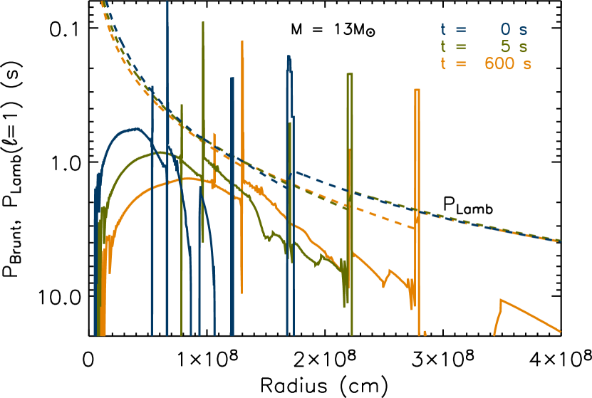
Figure 3: A time series of the propagation digram for the 13 M_☉ model from 600 s to 0 s before the start of collapse. $P_{Brunt}$ and $P_{Lamb}$ are defined as in Fig. 2. Notice that the evolution aburptly changes for $t=0$ s. This is due to the dramatic increase in nuclear rates during implosive burning, which causes new regions to become convective in the mixing-length calculation.

By prodigious neutrino emission, the cores of massive stars continue to change their structures prior to the onset of core collapse (Woosley et al. 2002). Figure 3 illustrates the changes of the propagation diagram for the 13 M_☉ model during the last ten minutes of evolution. As the inner regions quickly evolve and contract, the Brunt-Väisälä frequency increases with time, gradually increasing the modal frequencies. In contrast, the model corresponding to $t=0$ s (onset of collapse) exhibits a dramatic truncation in the size of the resonating cavity, in that $N^{2}$ drops to negative values as the convective region grows due to implosive burning. However, collapse happens on a dynamical timescale, and will take 200 to 250 ms. Given that the convective turnover times and the periods of oscillation are longer than this, the assumption of steady-state mixing-length convection is probably violated. Although for completeness, results for the $t=0$ s models are presented here, the quantitative results at $t=0$ s should be viewed with healthy skepticism. At other times, the structural changes are gradual enough for our peturbation theory to be reliable.

In this paper, the major sources and sinks of energy considered are nuclear burning, neutrino losses, and losses by coupling to outward propagating p-waves (Lai 2000b). Since losses by radiation is overwhelmed by neutrino emission, perturbations in the radiative flux is ignored. Throughout the Fe core, neutrino losses dominate over energy deposition. Only in the Si- and O-burning shells do nuclear reactions allow the $\epsilon$-mechanism to operate. For the typical g-mode with its largest amplitudes in the center, neutrino losses will dominate in eq. (21), resulting in stability. However, potentially unstable modes are those that are trapped mostly in the outer part of the core near or in the Si-burning region by the discontinuities in entropy, $Y_{e}$, and density (Lai 2000b).

4 Results

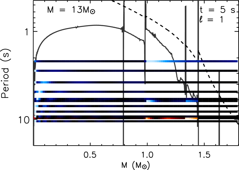
Figure 4: The propagation diagram for $\ell=1$ and the 13 M_☉ model at 5 s before the onset of collapse with $P_{Brunt}$ (solid) and $P_{Lamb}(\ell=1)$ (dashed), as defined in Fig. 2. The horizontal lines correspond to each eigenmode and period and are quantized. The shading in the lines is a measure of the magnitudes of the square of the amplitude, $|\xi|^{2}$. Within a single line brighter portions indicate a higher amplitude while the darker color signifies a lower amplitude. The blues indicate modes which are stable ($\tau<0$), and the reds correspond to the modes which are unstable ($\tau>0$).

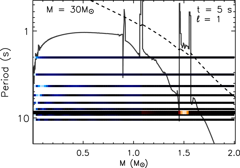
Figure 5: This figure is similar to Fig. 4, but for the 30 M_☉ model.

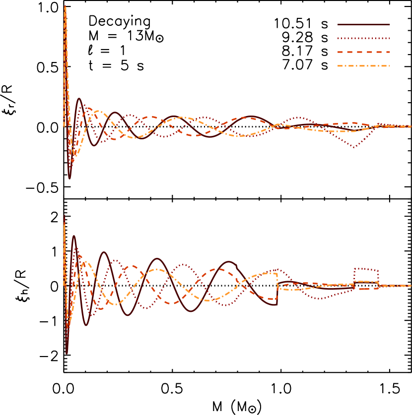
Figure 6: The dimensionless eigenfunctions of stable g-mode oscillations with periods of 10.51, 9.28, 8.17, and 7.07 s, for $\ell=1$, 13 M_☉, and 5 s before the start of collapse. Each mode is distinguished by its period. The top panel plots $\xi_{r}/R$, where $\xi_{r}$ is the radial component of perturbation and $R$ is the calculation domain size. The amplitude is arbitrarily scaled to 1.0 at its peak value. The bottom panel plots the corresponding horizontal amplitude, $\xi_{h}/R$.

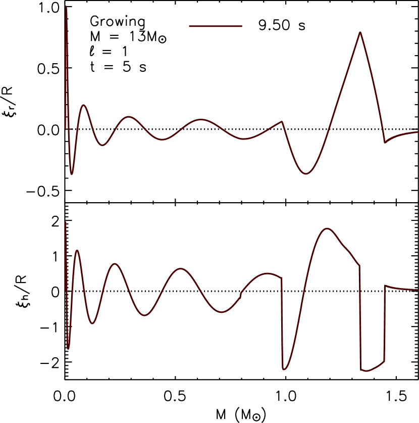
Figure 7: Plotted are the same attributes depicted in Fig. 6, but for a representative unstable mode with period 9.50 s.

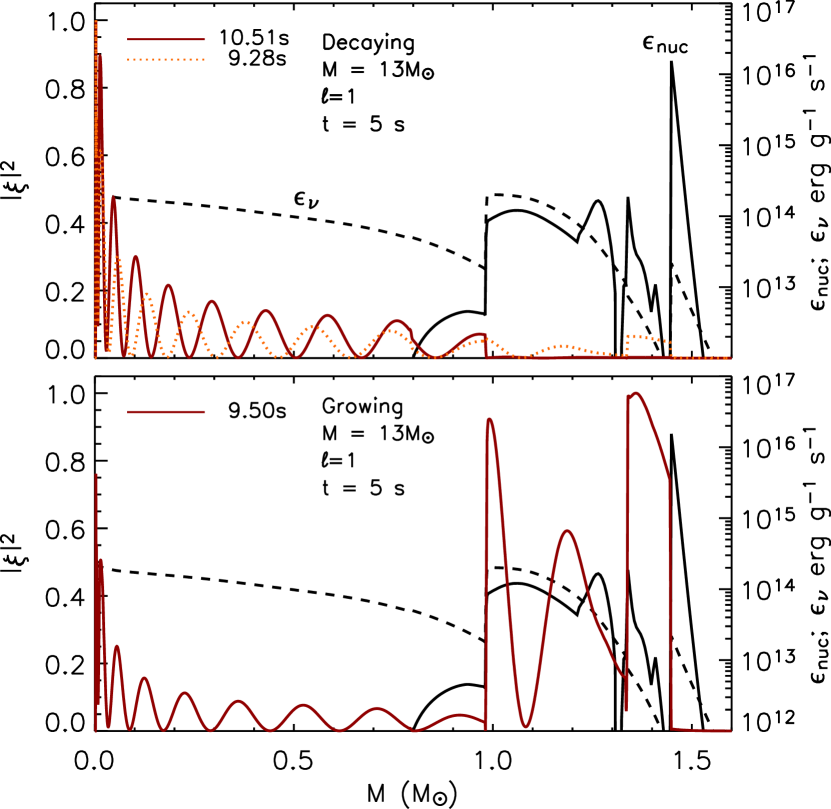
Figure 8: The Lagrangian displacement squared, $|\xi|^{2}$ (browns and oranges), the local deposition of energy by nuclear processes, $\epsilon_{nuc}$ (solid and black), and the local losses of energy due to neutrinos, $\epsilon_{\nu}$ (dashed), versus interior mass (M_☉) for the 13 M_☉ model, $\ell=1$, and 5 s before the onset of collapse. The top panel illustrates this comparison for two representative stable modes (periods = 10.51 and 9.28 s), while the bottom panel plots an unstable mode (period = 9.5 s). Note that the inner-core g-modes have their largest relative amplitudes where neutrino losses dominate, but that the outer-core g-modes have their largest relative amplitudes trapped in the recent Si burning ashes as well as the Si burning layer giving rise to instability.

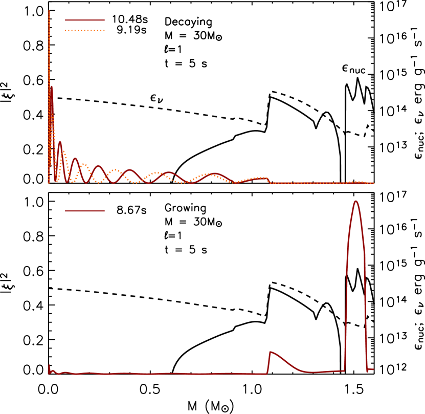
Figure 9: Same as Fig. 8, but for the $M=30$ M_☉ progenitor, stable modes with periods of 10.48 s and 9.19 s, and an unstable mode with period = 8.67 s.

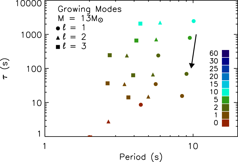
Figure 10: The growth timescales, $\tau$, in seconds, for the unstable modes versus their periods, in seconds, for the 13 M_☉ model. The plots are for $\ell=$ 1 (circle), 2 (triangle), and 3 (square) and for times of 60 (blue), 30, 25, 20, 15, 10, 5, 2, 1, and 0 (red) seconds before the onset of collapse. The arrow indicates the evolution of the period and growth timescales for particular modes as the models approach collapse.

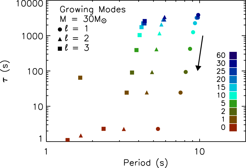
Figure 11: Same as Fig. 10, but for the $M=30$ M_☉ progenitor. Note the clear, uninterupted evolution of specific g-modes up to the onset of collapse.

The results of our analysis are summarized in Table 2, which lists all unstable modes found, and Figs. 4-11, which are described in detail below. Even though we did find modes for $\ell=$ 1, 2, 3, and higher $\ell$s, we present the results only for $\ell=$ 1, 2, and 3 in Table 2. since the trends at higher $\ell$s are adequatly demonstrated with the set presented in this paper. In general, the most interesting spherical harmonics to consider are those with odd $\ell$, or those with a top-bottom asymmetry. However even $\ell$s are interesting as well, as the nonlinear evolution of the perturbations into a kick may be triggered by any low order $\ell$. Since the dipole, $\ell=1$, spherical harmonic most closely resembles the desired kick geometry, we focus in this section on $\ell=1$, with peripheral mention of $\ell=2$ and 3.

Stable and unstable modes are found in all progenitor models. Figures 4 and 5 display the propagation diagram for the 13 M_☉ and 30 M_☉ models, at $t=5$ s before the commencement of collapse. These diagrams represent modes of the compact and extended profiles, respectively. Note again, the spikes resulting from $Y_{e}$ and $\rho$ discontinuities in $P_{Brunt}$ and the existence of a resonance cavity confined by O-shell convection in the 13 M_☉ model (Fig. 4). Because the O shell is farther out in mass for the more massive 30 M_☉ model (Fig. 5), the density and pressure profiles are more relevant in defining the resonant region. In both figures each horizontal line corresponds to a specific mode; the shading encodes $|\vec{\xi}|^{2}$. Dark and lighter shading signify low and high displacement, respectively, while blues denote stable modes and reds identify the unstable modes. Figures 4 and 5 show that there are many more stable modes than unstable modes, which is true for all models at all times and for all $\ell$s. We also identify two classes of g-modes, inner-core and outer-core g-modes. Inner-core g-modes have their greatest displacements toward the center and diminish with radius. Their spacing in $\log_{10}(Period)$ systematically decreases with increasing period and increasing number of half-wavelengths, $n$. In contrast outer-core g-modes do not have their greatest amplitude in the center. They are trapped by discontinuites between the fossil Fe core and the O shell in the case of the 13 M_☉ model and within the Si burning shell in the case of the 30 M_☉ model. Similar trapping exists for all other progenitors we consider.

Less than half of the outer-core g-modes are modes trapped entirely under the spikes (i.e. surface g-modes). While these modes satisfy the adiabatic linear oscillation equations, their physical significance is not well constrained. Their eigenfunctions and eigenfrequencies depend on the spike widths and heights, which in turn depend upon the interface between convective and radiative regions in mixing-length theory. However, the results and conclusions we present in this paper are not predicated on their character or existence.

A sample of inner-core g-modes for the 13 M_☉, $t=5$ s, model with $\ell=1$ is plotted versus interior mass in Fig. 6. The decreasing envelope of the eigenfunction and systematic increase in period with increasing half-wavelengths, $n$, is well explained by a WKB analysis (Unno et al. 1989). The quantization condition, $n\pi=\int k_{r}dr$, integrated over an appropriate resonant cavity, for g-waves gives

$$\omega_{R}=\frac{[\ell(\ell+1)]^{1/2}}{n\pi}\int_{cavity}\frac{N}{r}dr.$$ (25)

Numerically, the inner core frequencies are proportional to $[\ell(\ell+1)]^{1/2}/n$, and integrating eq. (25) over the appropriate resonance cavity gives approximately the same value. Following the conservation of wave flux arguments in Goldreich & Wu (1999), the envelope for the aribtrarily scaled amplitudes of $\xi_{r}/R$ and $\xi_{h}/R$ in Fig. 6 also correspond with those from the WKB analysis. In contrast, a simple WKB analysis fails to predict either the shape or the period of the outer-core g-mode shown in Fig 7. Instead, this mode’s period and large displacement farther out in mass are determined by both resonance in the overall cavity and resonant trapping between disontinuities in density, $Y_{e}$, and entropy.

In the context of losses and gains in energy, Fig. 8 displays $|\vec{\xi}|^{2}$ versus interior mass for two representative inner-core g-modes (top panel) and an outer-core g-mode (bottom panel) for the 13 $M_{\sun}$, $t=5$ s model for $\ell=1$, in addition to $\epsilon_{nuc}$ and $\epsilon_{\nu}$ in erg g^-1 s^-1. Figure 9 presents similar information for the 30 M_☉ model. The overlap of $|\vec{\xi}|^{2}$ with $\epsilon_{nuc}$ and $\epsilon_{\nu}$ is an excellent diagnostic proxy for the integrand in the work integral (eq. (18)). Clearly, neutrino losses dominate the work integral for the case of inner-core g-modes in both models. For the particular outer-core g-modes plotted for the 13 M_☉ and 30 $M_{\sun}$ progenitors in the bottom panels of Figs. 8 and 9, respectively, the large amplitude in the Si-burning region allows for instability. While all outer-core g-modes in Fig. 5 are unstable, two of the three 13 M_☉ outer-core g-modes in Fig. 4 are stablized by neutrino and acoustic losses. In general, at least one outer-core g-mode has the requisite radial perturbation distribution to be unstable.

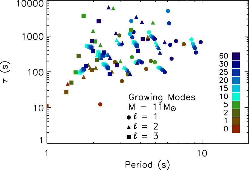
Figure 12: Same as Fig. 10 but for the $M=11$ M_☉ progenitor. While plenty of growing modes exist, their timescales are far too long for any significant growth to occur.

The growth timescales versus period for $\ell=$ 1, 2, and 3, $t=$ 60, 30, 25, 20, 15, 10, 5, 2, 1, and 0 s before the onset of collapse are plotted for 11 M_☉ 13 M_☉, and 30 M_☉ models in Figs. 12, 10, and 11, respectively. As expected, these figures illustrate that for higher $\ell$ the periods are smaller. Even though we find many unstable modes for the 11 M_☉ we do not find clear trends in the $\tau$ versus period plane. In contrast, as represented by the 13 M_☉ and 30 M_☉ models, all other masses we consider demonstrate a distinct trend. The arrows in Figs. 10 and 11 indicate the direction in which the modes evolve with time in the $\tau$ versus period plane. Specifically, later models are more compact and have shorter period oscillations. In addition, the later, more compact, models have slightly higher densities and temperatures in the burning regions, thereby dramatically increasing the burning rates and decreasing $\tau$ in Figs. 10 and 11. Also note that at no point in any of the models are the growth timescales shorter than the times until the start of collapse. These trends continue to the onset of collapse, which is marked on Figs. 10 and 11 with red symbols. In fact, for the latest models, $t=0$ s and 1 s before the start of collapse, $\tau$ becomes comparable to the period, calling into question the assumption in §2.1 of small nonadiabatic effects. While dramatic changes imposed by dynamical collapse and implosive burning for the $t=0$ s models make the effects listed above more pronounced, the qualitative trends highlighted still obtain for the $t=0$ s models.

For all unstable modes found Table 2 lists the progenitor mass, time until onset of collapse, the period, growth timescale, $\tau$, and the contributions, $\tau_{nuc}$, $\tau_{\nu}$, and $\tau_{leak}$. From tens of minutes before commencement of collapse until collapse itself, unstable modes exist in all progenitor models. However, at every evolutionary stage the timescale for growth is an order-of-magnitude or two longer than the time until onset of collapse. The rates of growth or decay we derive are too long compared to the time to onset of collapse to significantly alter the mode amplitudes. It seems that even though the $\epsilon$-mechanism is present in the later evolutionary stages of the cores of massive stars, the timescales imply that its effect is not large.

4.1 Analytic Estimates

Consistently, we find that the timescales for growth are longer than the time until the onset of collapse. As such the $\epsilon$-mechanism is not able to significantly affect the amplitudes of the unstable g-modes. Hence, our evaluation of the succesfulness of the $\epsilon$-mechanism depends upon the validity of the timescale calculations. In this section we corroborate, with an analytic estimate for $\tau_{nuc}$, our numerical evaluations for the growth timescales.

$W_{j}$, given by eq. (18), is the rate of energy gained or lost, and $E_{W}$, eq. (23), is the energy in the mode. Assuming the region where nuclear burning interacts with a growing mode is small and the mode itself may be represented by a top-hat function located entirely and only within the burning region with maximum displacement $\Delta r/r$, then the integrand in eq. (18) is roughly constant. Therefore,

$$W_{j}\sim\frac{\pi}{\omega_{R}}\epsilon_{j}\epsilon_{jT}\left(\frac{\delta T}{T}\right)^{2}\frac{\Delta M}{4\pi},$$ (26)

and eq. (19), simplifies to

$$\frac{\delta T}{T}\sim V\nabla_{ad}\left(\frac{\Delta r}{r}\right).$$ (27)

As a harmonic oscillation, g-modes are the oscillations of isodensity contours about their equilibrium positions in hydrostatic equilibrium. The harmonic potential is $U\sim\text@frac{1}{2}\partial^{2}\phi_{eff}/\partial r^{2}x^{2}$, where $x=\Delta re^{i\omega t}$. From $\vec{\nabla}\phi=\vec{\nabla}P/\rho$, we get $\phi_{eff}\sim\phi\sim P/\rho\sim GM_{r}/r$. Hence, the potential energy, $u$, is given by

$$u\sim\frac{GM_{r}}{r}\left(\frac{x}{r}\right)^{2}.$$ (28)

Since $E_{W}=2\int<u>dM_{r}$, where $<>$ denotes the time average over one period of oscillation, then

$$E_{W}\sim\frac{GM_{r}}{r}\left(\frac{\Delta r}{r}\right)^{2}\frac{\Delta M}{4\pi}.$$ (29)

Finally, taking the ratio of eq. (29) and eq. (26) gives a rough estimate for $\tau$:

$$\tau_{nuc}=\frac{4\pi E_{W}}{\omega_{R}W_{nuc}}\sim 4\frac{P/(\rho V)}{\epsilon_{nuc}\epsilon_{nucT}\nabla_{ad}^{2}},$$ (30)

In the burning region, for the 30 M_☉ $t=5$ s model and the 8.67 s, $\ell=1$ mode, $P/\rho\sim 2.2\times 10^{17}$ erg g^-1, $\epsilon_{nuc}\epsilon_{nucT}\sim 2\times 10^{16}$ erg g^-1 s^-1, $\nabla_{ad}\sim 1/4$, and $V\sim 2$, giving $\tau_{nuc}\sim 320$ s from eq. (30). The numerical solution in Table 2 is $\tau_{nuc}=328$ s. Similarly for the 8.45 s, $\ell=1$ mode of the 13 M_☉ progenitor model at $t=1$ s, $P/\rho\sim 1.4\times 10^{17}$ erg g^-1, $\epsilon_{nuc}\epsilon_{nucT}\sim 10^{17}$ erg g^-1 s^-1, $\nabla_{ad}\sim 1/4$, and $V\sim 3$, giving $\tau_{nuc}\sim 30$ s from eq.(30). The numerical solution (Table 2) is $\tau_{nuc}=15.5$ s. That the simple analytic arguments and estimates approximately reproduce the numerical results is reassuring. Even though the nuclear rates increase toward later times, at no time is this trend enough to cause significant growth prior to collapse.

5 Summary and Conclusions

For all progenitors, we find stable and unstable g-modes with oscillation periods in the range from $\sim$1 to $\sim$10 seconds. The stable g-modes are often concentrated in the inner core and are stabilized by neutrino emission. Unstable g-modes on the other hand are trapped in the outer radii of the core by discontinuities in $S$, density, and $Y_{e}$. Their typical growth timescales determined numerically and analytically range from 10s to 10,000s of seconds, which are long compared to the time until the start of collapse. Therefore, we conclude that the $\epsilon$-mechanism is an unlikely source for large perturbations in the progenitor prior to the onset of collapse.

There are several caveats to our conclusion. Our results are for a set of 1-D nonrotating models from Rauscher et al. (2002) and Woosley et al. (2002). Rotation in the late stages of massive stellar evolution may significantly effect the structure of the star prior to collapse (Heger, Langer, & Woosley 2000; Heger, Woosley, & Langer 2003), thereby altering the analysis in this paper. However, with modest Fe core rotation periods ($\gtrsim 10$ s) we expect little deviation from our results, and the simple energy arguments in §4.1 should hold. We also have not considered a different suite of progenitor models (Nomoto & Hashimoto 1988; Limongi & Chieffi 2003), which may have different eigenmodes. In addition, calculating full 3-D, non-linear, dynamical convection with nuclear reactions during the final stages of massive star evolution is a task for the future; the progenitors and their g-modes may be significantly different than assumed or calculated here.

We also have not considered coupling between convective modes and g-modes, which provides an excellent mechanism for the excitation of the 5-minute p-modes in the Sun (Goldreich & Kumar 1990). In such analyses, the amplitudes of the modes are estimated by assuming steady state is achieved in the nonlinear time-dependent amplitude equations. However, the short timescales until the onset of collapse would violate the assumption of steady state and invalidate such analyses. More importantly, it would be unlikely that the short timescales until the onset of collapse would allow for significant excitation of g-modes by convection.

On the other hand, the growth of perturbations in the supersonic regions during collapse does occur (Lai 2000a; Lai & Goldreich 2000). Because we have not ruled out all possible sources of perturbations prior to collapse, asymmetries in the progenitor may still be relevant in producing the largest kicks. For example, convection in the last stages of evolution is often quite vigorous and may have Mach numbers in the range 0.1 to 0.2 and density perturbations, $\delta\rho/\rho$, in the range 0.01 to 0.05 (Bazan & Arnett 1998). These perturbations may indeed be sufficient to produce the observed kicks (Burrows & Hayes 1996).

In performing a stellar pulsational and stability analysis of the late-time cores of massive stars, we have identified many stable and unstable modes. We note that stability is predominantly determined by the neutrino losses or energy deposition by nuclear reactions. Compared with the time until the onset of collapse, the timescales for growth and decay are long. In §4.1, we argue that the long growth timescales (compared with the time until the start of collapse) are confirmed by energetic arguments. We suggest that the $\epsilon$-mechanism for g-mode growth does not generate the requisite perturbations prior to collapse needed to stimulate large kicks during the supernova explosion. Therefore, we conclude that if the hydrodynamic mechanism in combination with progenitor perturbations is to succeed in explaining neutron star kicks other sources of seed perturbations must be investigated.

Table 1: Structural Boundaries

Mass (M☉)	Fossil Core (M☉)	Fe Core (M☉)	O Base (M☉)
11	0.83	1.22 (C)	1.36(C)
13	0.98	1.33 (R)	1.44(C)
15	1.05	1.41 (R)	1.74(C)
20	0.99	1.46 (R)	1.60(C)
30	1.06	1.45 (R)	2.03(C)
35	0.96	1.47 (M)	1.66(C)
40	0.97	1.54 (R)	1.76(C)

Table 2: Growing Modes

Mass (M☉)	t (s)	Period (s)	$\tau$ (s)	$1/\tau_{nuc}$ (s-1)	$-1/\tau_{\nu}$ (s-1)	$-1/\tau_{leak}$ (s-1)
$\ell=1$
11	0	2.21	$1.23\times 10^{1}$	$1.60\times 10^{-1}$	$6.66\times 10^{-2}$	$1.23\times 10^{-2}$
-	1	7.63	$5.93\times 10^{2}$	$6.62\times 10^{-3}$	$4.93\times 10^{-3}$	$\sim 0$
-	1	4.37	$1.20\times 10^{2}$	$1.52\times 10^{-2}$	$6.87\times 10^{-3}$	$2.20\times 10^{-5}$
-	1	3.04	$5.49\times 10^{1}$	$2.87\times 10^{-2}$	$6.40\times 10^{-3}$	$4.12\times 10^{-3}$
-	1	2.74	$1.86\times 10^{2}$	$2.56\times 10^{-2}$	$6.30\times 10^{-3}$	$1.39\times 10^{-2}$
-	5	4.97	$1.85\times 10^{2}$	$7.09\times 10^{-3}$	$1.68\times 10^{-3}$	$1.56\times 10^{-5}$
-	5	3.53	$2.56\times 10^{2}$	$7.96\times 10^{-3}$	$2.02\times 10^{-3}$	$2.03\times 10^{-3}$
-	30	9.14	$3.47\times 10^{2}$	$3.79\times 10^{-3}$	$9.07\times 10^{-4}$	$\sim 0$
-	30	6.24	$5.69\times 10^{2}$	$3.07\times 10^{-3}$	$1.31\times 10^{-3}$	$\sim 0$
-	30	5.75	$9.77\times 10^{1}$	$1.11\times 10^{-2}$	$8.26\times 10^{-4}$	$\sim 0$
-	30	4.96	$8.20\times 10^{2}$	$2.68\times 10^{-3}$	$1.44\times 10^{-3}$	$1.87\times 10^{-5}$
-	30	4.09	$1.83\times 10^{2}$	$7.23\times 10^{-3}$	$9.63\times 10^{-4}$	$8.07\times 10^{-4}$
-	30	3.62	$1.30\times 10^{3}$	$4.14\times 10^{-3}$	$1.15\times 10^{-3}$	$2.22\times 10^{-3}$
-	60	9.80	$6.74\times 10^{2}$	$2.09\times 10^{-3}$	$6.11\times 10^{-4}$	$\sim 0$
-	60	6.80	$7.24\times 10^{2}$	$2.19\times 10^{-3}$	$8.11\times 10^{-4}$	$\sim 0$
-	60	6.37	$2.34\times 10^{2}$	$4.89\times 10^{-3}$	$6.15\times 10^{-4}$	$\sim 0$
-	60	4.48	$8.15\times 10^{2}$	$2.36\times 10^{-3}$	$6.85\times 10^{-4}$	$4.50\times 10^{-4}$
13	0	4.44	$8.59\times 10^{0}$	$2.54\times 10^{-1}$	$1.37\times 10^{-1}$	$6.46\times 10^{-6}$
-	0	4.34	$4.70\times 10^{-1}$	$2.15\times 10^{0}$	$2.32\times 10^{-2}$	$9.40\times 10^{-5}$
-	1	8.42	$1.55\times 10^{1}$	$6.65\times 10^{-2}$	$2.19\times 10^{-3}$	$4.82\times 10^{-6}$
-	1	5.59	$3.47\times 10^{1}$	$3.24\times 10^{-2}$	$3.38\times 10^{-3}$	$1.42\times 10^{-4}$
-	5	9.50	$7.90\times 10^{2}$	$2.32\times 10^{-3}$	$1.05\times 10^{-3}$	$4.20\times 10^{-6}$
15	0	4.59	$7.13\times 10^{-1}$	$1.43\times 10^{0}$	$1.54\times 10^{-3}$	$2.61\times 10^{-2}$
-	1	8.39	$3.15\times 10^{1}$	$3.18\times 10^{-2}$	$6.32\times 10^{-5}$	$\sim 0$
-	1	5.23	$5.64\times 10^{1}$	$5.02\times 10^{-2}$	$6.05\times 10^{-4}$	$3.19\times 10^{-2}$
-	5	8.66	$1.37\times 10^{2}$	$7.35\times 10^{-3}$	$4.82\times 10^{-5}$	$\sim 0$
-	30	9.15	$4.43\times 10^{2}$	$2.30\times 10^{-3}$	$3.88\times 10^{-5}$	$\sim 0$
-	30	6.62	$9.75\times 10^{2}$	$1.42\times 10^{-3}$	$3.93\times 10^{-4}$	$\sim 0$
-	60	9.52	$6.31\times 10^{2}$	$1.63\times 10^{-3}$	$4.40\times 10^{-5}$	$\sim 0$
-	60	7.03	$9.44\times 10^{2}$	$1.45\times 10^{-3}$	$3.92\times 10^{-4}$	$\sim 0$
-	600	11.04	$9.68\times 10^{5}$	$6.84\times 10^{-5}$	$6.73\times 10^{-5}$	$\sim 0$
-	3600	24.28	$5.48\times 10^{4}$	$7.68\times 10^{-5}$	$5.86\times 10^{-5}$	$\sim 0$
-	3600	16.47	$9.99\times 10^{4}$	$5.89\times 10^{-5}$	$4.89\times 10^{-5}$	$\sim 0$
-	3600	13.00	$3.40\times 10^{5}$	$2.40\times 10^{-5}$	$2.11\times 10^{-5}$	$\sim 0$
20	1	10.03	$3.61\times 10^{1}$	$2.94\times 10^{-2}$	$1.65\times 10^{-3}$	$1.95\times 10^{-5}$
-	1	6.77	$1.77\times 10^{2}$	$9.49\times 10^{-3}$	$3.68\times 10^{-3}$	$1.43\times 10^{-4}$
-	5	11.14	$2.91\times 10^{2}$	$4.18\times 10^{-3}$	$7.44\times 10^{-4}$	$5.11\times 10^{-6}$
25	0	5.86	$7.29\times 10^{-1}$	$1.38\times 10^{0}$	$4.03\times 10^{-3}$	$\sim 0$
-	1	10.70	$2.89\times 10^{1}$	$3.79\times 10^{-2}$	$3.27\times 10^{-3}$	$\sim 0$
-	1	7.09	$1.74\times 10^{1}$	$5.96\times 10^{-2}$	$2.20\times 10^{-3}$	$\sim 0$
-	1	6.74	$1.17\times 10^{2}$	$1.34\times 10^{-2}$	$4.85\times 10^{-3}$	$\sim 0$
-	5	11.30	$3.97\times 10^{2}$	$3.91\times 10^{-3}$	$1.39\times 10^{-3}$	$\sim 0$
-	5	7.88	$2.54\times 10^{2}$	$5.04\times 10^{-3}$	$1.10\times 10^{-3}$	$\sim 0$
-	30	8.71	$2.59\times 10^{3}$	$1.12\times 10^{-3}$	$7.33\times 10^{-4}$	$\sim 0$
-	60	9.18	$1.01\times 10^{4}$	$7.30\times 10^{-4}$	$6.31\times 10^{-4}$	$\sim 0$
-	3600	17.25	$8.35\times 10^{5}$	$6.13\times 10^{-5}$	$6.01\times 10^{-5}$	$\sim 0$
30	0	5.35	$2.28\times 10^{0}$	$4.41\times 10^{-1}$	$3.31\times 10^{-3}$	$\sim 0$
-	1	7.51	$2.44\times 10^{1}$	$4.18\times 10^{-2}$	$8.26\times 10^{-4}$	$\sim 0$
-	5	8.67	$4.23\times 10^{2}$	$3.04\times 10^{-3}$	$6.76\times 10^{-4}$	$\sim 0$
-	30	9.79	$3.84\times 10^{3}$	$7.83\times 10^{-4}$	$5.23\times 10^{-4}$	$\sim 0$
-	3600	16.13	$5.74\times 10^{6}$	$3.21\times 10^{-5}$	$3.20\times 10^{-5}$	$\sim 0$
35	0	5.09	$3.49\times 10^{1}$	$9.27\times 10^{-2}$	$6.41\times 10^{-2}$	$1.49\times 10^{-5}$
-	0	4.82	$5.28\times 10^{-1}$	$1.90\times 10^{0}$	$6.93\times 10^{-3}$	$1.08\times 10^{-3}$
-	1	7.99	$1.81\times 10^{2}$	$8.57\times 10^{-3}$	$3.05\times 10^{-3}$	$\sim 0$
-	1	7.60	$1.35\times 10^{2}$	$1.06\times 10^{-2}$	$3.16\times 10^{-3}$	$\sim 0$
-	1	5.85	$5.22\times 10^{1}$	$2.14\times 10^{-2}$	$2.20\times 10^{-3}$	$\sim 0$
-	5	8.36	$9.90\times 10^{2}$	$2.06\times 10^{-3}$	$1.05\times 10^{-3}$	$\sim 0$
-	5	6.44	$1.09\times 10^{3}$	$2.14\times 10^{-3}$	$1.22\times 10^{-3}$	$\sim 0$
-	30	9.19	$5.03\times 10^{3}$	$7.07\times 10^{-4}$	$5.09\times 10^{-4}$	$\sim 0$
-	60	9.70	$6.22\times 10^{3}$	$5.61\times 10^{-4}$	$4.00\times 10^{-4}$	$\sim 0$
40	0	5.95	$5.45\times 10^{1}$	$6.82\times 10^{-2}$	$4.98\times 10^{-2}$	$1.83\times 10^{-5}$
-	0	5.47	$5.43\times 10^{-1}$	$1.85\times 10^{0}$	$7.20\times 10^{-3}$	$1.55\times 10^{-3}$
-	1	9.00	$7.88\times 10^{1}$	$1.60\times 10^{-2}$	$3.31\times 10^{-3}$	$\sim 0$
-	1	8.56	$3.63\times 10^{1}$	$3.03\times 10^{-2}$	$2.81\times 10^{-3}$	$\sim 0$
-	1	7.39	$4.46\times 10^{3}$	$4.74\times 10^{-3}$	$4.51\times 10^{-3}$	$\sim 0$
-	1	6.36	$5.41\times 10^{1}$	$2.24\times 10^{-2}$	$3.47\times 10^{-3}$	$5.00\times 10^{-4}$
-	1	5.95	$5.62\times 10^{1}$	$2.23\times 10^{-2}$	$3.36\times 10^{-3}$	$1.11\times 10^{-3}$
-	5	9.45	$6.06\times 10^{2}$	$2.55\times 10^{-3}$	$8.97\times 10^{-4}$	$\sim 0$
$\ell=2$
11	0	1.36	$4.55\times 10^{1}$	$1.19\times 10^{-1}$	$8.66\times 10^{-2}$	$9.96\times 10^{-3}$
-	1	4.47	$9.37\times 10^{2}$	$6.07\times 10^{-3}$	$5.00\times 10^{-3}$	$\sim 0$
-	1	2.63	$1.02\times 10^{2}$	$1.57\times 10^{-2}$	$5.87\times 10^{-3}$	$1.19\times 10^{-5}$
-	1	1.90	$1.28\times 10^{2}$	$1.75\times 10^{-2}$	$7.99\times 10^{-3}$	$1.67\times 10^{-3}$
-	1	1.73	$7.23\times 10^{1}$	$3.58\times 10^{-2}$	$4.37\times 10^{-3}$	$1.76\times 10^{-2}$
-	5	4.82	$2.40\times 10^{3}$	$2.28\times 10^{-3}$	$1.86\times 10^{-3}$	$\sim 0$
-	5	2.98	$1.98\times 10^{2}$	$6.66\times 10^{-3}$	$1.59\times 10^{-3}$	$1.11\times 10^{-5}$
-	5	2.68	$6.02\times 10^{3}$	$2.93\times 10^{-3}$	$2.74\times 10^{-3}$	$2.73\times 10^{-5}$
-	5	2.21	$5.67\times 10^{2}$	$4.89\times 10^{-3}$	$2.40\times 10^{-3}$	$7.25\times 10^{-4}$
-	5	1.98	$1.41\times 10^{3}$	$1.15\times 10^{-2}$	$1.31\times 10^{-3}$	$9.52\times 10^{-3}$
-	30	5.35	$3.45\times 10^{2}$	$3.77\times 10^{-3}$	$8.73\times 10^{-4}$	$\sim 0$
-	30	3.77	$3.43\times 10^{3}$	$1.70\times 10^{-3}$	$1.41\times 10^{-3}$	$\sim 0$
-	30	3.44	$8.76\times 10^{1}$	$1.21\times 10^{-2}$	$7.12\times 10^{-4}$	$\sim 0$
-	30	3.07	$6.34\times 10^{2}$	$2.98\times 10^{-3}$	$1.39\times 10^{-3}$	$1.02\times 10^{-5}$
-	30	2.55	$2.50\times 10^{2}$	$5.46\times 10^{-3}$	$1.11\times 10^{-3}$	$3.54\times 10^{-4}$
-	30	2.29	$2.94\times 10^{2}$	$6.24\times 10^{-3}$	$9.68\times 10^{-4}$	$1.87\times 10^{-3}$
-	60	5.74	$6.82\times 10^{2}$	$2.08\times 10^{-3}$	$6.13\times 10^{-4}$	$\sim 0$
-	60	4.10	$2.49\times 10^{3}$	$1.30\times 10^{-3}$	$8.98\times 10^{-4}$	$\sim 0$
-	60	3.82	$1.81\times 10^{2}$	$6.04\times 10^{-3}$	$5.00\times 10^{-4}$	$\sim 0$
-	60	2.78	$1.21\times 10^{3}$	$1.79\times 10^{-3}$	$7.59\times 10^{-4}$	$2.04\times 10^{-4}$
-	60	2.50	$6.38\times 10^{3}$	$1.79\times 10^{-3}$	$7.31\times 10^{-4}$	$8.98\times 10^{-4}$
13	0	2.68	$2.77\times 10^{0}$	$4.87\times 10^{-1}$	$1.26\times 10^{-1}$	$9.02\times 10^{-6}$
-	0	2.65	$5.43\times 10^{-1}$	$1.88\times 10^{0}$	$3.80\times 10^{-2}$	$4.10\times 10^{-5}$
-	1	4.99	$1.49\times 10^{1}$	$6.93\times 10^{-2}$	$2.10\times 10^{-3}$	$1.89\times 10^{-6}$
-	1	3.44	$3.46\times 10^{1}$	$3.24\times 10^{-2}$	$3.41\times 10^{-3}$	$6.10\times 10^{-5}$
-	5	5.64	$7.10\times 10^{2}$	$2.41\times 10^{-3}$	$9.96\times 10^{-4}$	$2.04\times 10^{-6}$
15	0	2.85	$6.14\times 10^{-1}$	$1.64\times 10^{0}$	$1.25\times 10^{-3}$	$7.38\times 10^{-3}$
-	0	1.79	$1.01\times 10^{1}$	$1.76\times 10^{-1}$	$6.39\times 10^{-2}$	$1.35\times 10^{-2}$
-	0	1.72	$3.76\times 10^{0}$	$3.35\times 10^{-1}$	$3.67\times 10^{-2}$	$3.26\times 10^{-2}$
-	1	6.16	$5.42\times 10^{1}$	$1.85\times 10^{-2}$	$3.28\times 10^{-5}$	$\sim 0$
-	1	3.24	$1.89\times 10^{1}$	$6.47\times 10^{-2}$	$4.80\times 10^{-4}$	$1.14\times 10^{-2}$
-	5	6.34	$1.75\times 10^{2}$	$5.76\times 10^{-3}$	$2.55\times 10^{-5}$	$\sim 0$
-	60	4.34	$1.10\times 10^{3}$	$1.24\times 10^{-3}$	$3.28\times 10^{-4}$	$\sim 0$
-	3600	14.17	$6.48\times 10^{4}$	$7.16\times 10^{-5}$	$5.62\times 10^{-5}$	$\sim 0$
-	3600	10.32	$1.58\times 10^{5}$	$2.71\times 10^{-5}$	$2.08\times 10^{-5}$	$\sim 0$
-	3600	9.11	$1.73\times 10^{5}$	$4.80\times 10^{-5}$	$4.22\times 10^{-5}$	$\sim 0$
20	1	6.04	$3.50\times 10^{1}$	$3.02\times 10^{-2}$	$1.65\times 10^{-3}$	$9.49\times 10^{-6}$
-	1	4.19	$3.43\times 10^{2}$	$7.12\times 10^{-3}$	$4.15\times 10^{-3}$	$4.97\times 10^{-5}$
25	0	2.38	$2.85\times 10^{0}$	$4.67\times 10^{-1}$	$7.70\times 10^{-4}$	$1.16\times 10^{-1}$
-	1	6.43	$3.07\times 10^{1}$	$3.59\times 10^{-2}$	$3.39\times 10^{-3}$	$\sim 0$
-	1	4.43	$1.52\times 10^{1}$	$6.78\times 10^{-2}$	$1.87\times 10^{-3}$	$\sim 0$
-	1	4.24	$2.20\times 10^{2}$	$9.57\times 10^{-3}$	$5.02\times 10^{-3}$	$\sim 0$
-	5	6.58	$1.21\times 10^{3}$	$2.49\times 10^{-3}$	$1.67\times 10^{-3}$	$\sim 0$
-	5	4.91	$2.32\times 10^{2}$	$5.39\times 10^{-3}$	$1.07\times 10^{-3}$	$\sim 0$
-	30	5.41	$1.56\times 10^{3}$	$1.17\times 10^{-3}$	$5.28\times 10^{-4}$	$\sim 0$
-	60	5.70	$8.32\times 10^{3}$	$7.60\times 10^{-4}$	$6.40\times 10^{-4}$	$\sim 0$
-	3600	4.59	$4.81\times 10^{4}$	$3.23\times 10^{-5}$	$1.15\times 10^{-5}$	$\sim 0$
30	0	3.20	$2.27\times 10^{0}$	$4.41\times 10^{-1}$	$1.12\times 10^{-3}$	$\sim 0$
-	0	1.68	$1.49\times 10^{0}$	$7.94\times 10^{-1}$	$2.55\times 10^{-3}$	$1.21\times 10^{-1}$
-	1	4.52	$2.47\times 10^{1}$	$4.12\times 10^{-2}$	$6.75\times 10^{-4}$	$\sim 0$
-	5	5.23	$4.11\times 10^{2}$	$3.01\times 10^{-3}$	$5.74\times 10^{-4}$	$\sim 0$
-	30	5.91	$3.37\times 10^{3}$	$7.55\times 10^{-4}$	$4.58\times 10^{-4}$	$\sim 0$
35	0	2.98	$4.93\times 10^{-1}$	$2.03\times 10^{0}$	$5.28\times 10^{-3}$	$6.57\times 10^{-4}$
-	1	4.77	$2.31\times 10^{2}$	$7.53\times 10^{-3}$	$3.20\times 10^{-3}$	$\sim 0$
-	1	4.56	$1.34\times 10^{2}$	$1.06\times 10^{-2}$	$3.15\times 10^{-3}$	$\sim 0$
-	1	3.63	$5.13\times 10^{1}$	$2.17\times 10^{-2}$	$2.23\times 10^{-3}$	$\sim 0$
-	1	3.41	$2.01\times 10^{3}$	$4.80\times 10^{-3}$	$4.30\times 10^{-3}$	$\sim 0$
-	5	5.00	$8.02\times 10^{2}$	$2.24\times 10^{-3}$	$9.89\times 10^{-4}$	$\sim 0$
-	5	3.99	$1.45\times 10^{3}$	$1.96\times 10^{-3}$	$1.27\times 10^{-3}$	$\sim 0$
-	30	5.49	$4.08\times 10^{3}$	$7.37\times 10^{-4}$	$4.92\times 10^{-4}$	$\sim 0$
-	60	5.79	$4.78\times 10^{3}$	$5.93\times 10^{-4}$	$3.84\times 10^{-4}$	$\sim 0$
40	0	3.44	$5.12\times 10^{-1}$	$1.96\times 10^{0}$	$6.00\times 10^{-3}$	$7.37\times 10^{-4}$
-	0	2.04	$1.14\times 10^{1}$	$2.73\times 10^{-1}$	$1.27\times 10^{-3}$	$1.83\times 10^{-1}$
-	1	5.37	$7.42\times 10^{1}$	$1.68\times 10^{-2}$	$3.32\times 10^{-3}$	$\sim 0$
-	1	5.14	$3.53\times 10^{1}$	$3.11\times 10^{-2}$	$2.85\times 10^{-3}$	$\sim 0$
-	1	3.99	$6.50\times 10^{1}$	$1.94\times 10^{-2}$	$3.74\times 10^{-3}$	$2.70\times 10^{-4}$
-	1	3.75	$4.21\times 10^{1}$	$2.75\times 10^{-2}$	$2.95\times 10^{-3}$	$8.16\times 10^{-4}$
-	5	5.68	$5.29\times 10^{2}$	$2.75\times 10^{-3}$	$8.57\times 10^{-4}$	$\sim 0$
$\ell=3$
11	0	0.99	$1.10\times 10^{1}$	$1.63\times 10^{-1}$	$5.81\times 10^{-2}$	$1.35\times 10^{-2}$
-	0	0.88	$3.74\times 10^{0}$	$4.71\times 10^{-1}$	$1.03\times 10^{-2}$	$1.94\times 10^{-1}$
-	1	1.95	$1.12\times 10^{2}$	$1.42\times 10^{-2}$	$5.20\times 10^{-3}$	$2.74\times 10^{-6}$
-	1	1.33	$2.69\times 10^{1}$	$4.67\times 10^{-2}$	$3.09\times 10^{-3}$	$6.43\times 10^{-3}$
-	5	3.49	$1.49\times 10^{3}$	$2.34\times 10^{-3}$	$1.66\times 10^{-3}$	$\sim 0$
-	5	2.21	$2.90\times 10^{2}$	$5.19\times 10^{-3}$	$1.73\times 10^{-3}$	$1.77\times 10^{-6}$
-	5	2.04	$7.05\times 10^{2}$	$3.85\times 10^{-3}$	$2.43\times 10^{-3}$	$6.93\times 10^{-6}$
-	5	1.72	$3.69\times 10^{3}$	$2.98\times 10^{-3}$	$2.63\times 10^{-3}$	$8.16\times 10^{-5}$
-	5	1.53	$9.65\times 10^{1}$	$1.46\times 10^{-2}$	$1.06\times 10^{-3}$	$3.19\times 10^{-3}$
-	30	3.86	$3.89\times 10^{2}$	$3.45\times 10^{-3}$	$8.84\times 10^{-4}$	$\sim 0$
-	30	2.54	$8.66\times 10^{1}$	$1.22\times 10^{-2}$	$6.88\times 10^{-4}$	$\sim 0$
-	30	2.34	$3.47\times 10^{2}$	$4.18\times 10^{-3}$	$1.30\times 10^{-3}$	$\sim 0$
-	30	1.98	$3.78\times 10^{2}$	$3.92\times 10^{-3}$	$1.22\times 10^{-3}$	$4.68\times 10^{-5}$
-	30	1.79	$1.43\times 10^{2}$	$8.31\times 10^{-3}$	$8.23\times 10^{-4}$	$4.93\times 10^{-4}$
-	60	4.15	$8.29\times 10^{2}$	$1.86\times 10^{-3}$	$6.54\times 10^{-4}$	$\sim 0$
-	60	2.83	$1.53\times 10^{2}$	$6.97\times 10^{-3}$	$4.27\times 10^{-4}$	$\sim 0$
-	60	2.56	$5.36\times 10^{4}$	$9.63\times 10^{-4}$	$9.45\times 10^{-4}$	$\sim 0$
-	60	2.16	$2.59\times 10^{3}$	$1.23\times 10^{-3}$	$8.23\times 10^{-4}$	$2.29\times 10^{-5}$
-	60	1.95	$7.26\times 10^{2}$	$2.24\times 10^{-3}$	$6.45\times 10^{-4}$	$2.18\times 10^{-4}$
13	0	2.02	$9.43\times 10^{-1}$	$1.14\times 10^{0}$	$8.20\times 10^{-2}$	$3.31\times 10^{-6}$
-	0	2.01	$9.39\times 10^{-1}$	$1.15\times 10^{0}$	$8.29\times 10^{-2}$	$3.63\times 10^{-6}$
-	0	2.01	$9.39\times 10^{-1}$	$1.15\times 10^{0}$	$8.29\times 10^{-2}$	$3.63\times 10^{-6}$
-	1	3.66	$1.41\times 10^{1}$	$7.29\times 10^{-2}$	$1.99\times 10^{-3}$	$3.30\times 10^{-7}$
-	1	2.65	$3.66\times 10^{1}$	$3.09\times 10^{-2}$	$3.53\times 10^{-3}$	$7.66\times 10^{-6}$
-	5	4.14	$6.59\times 10^{2}$	$2.47\times 10^{-3}$	$9.52\times 10^{-4}$	$3.54\times 10^{-7}$
15	0	2.21	$5.65\times 10^{-1}$	$1.77\times 10^{0}$	$1.06\times 10^{-3}$	$1.26\times 10^{-3}$
-	0	1.42	$3.08\times 10^{1}$	$1.02\times 10^{-1}$	$6.84\times 10^{-2}$	$1.45\times 10^{-3}$
-	0	1.38	$4.50\times 10^{0}$	$2.57\times 10^{-1}$	$3.07\times 10^{-2}$	$4.45\times 10^{-3}$
-	1	2.49	$1.31\times 10^{1}$	$7.92\times 10^{-2}$	$3.38\times 10^{-4}$	$2.56\times 10^{-3}$
-	1	1.67	$2.17\times 10^{1}$	$5.90\times 10^{-2}$	$1.34\times 10^{-3}$	$1.16\times 10^{-2}$
-	5	2.76	$1.89\times 10^{2}$	$7.16\times 10^{-3}$	$2.20\times 10^{-4}$	$1.64\times 10^{-3}$
-	30	3.06	$1.05\times 10^{3}$	$1.22\times 10^{-3}$	$2.67\times 10^{-4}$	$\sim 0$
-	60	3.26	$1.07\times 10^{3}$	$1.20\times 10^{-3}$	$2.67\times 10^{-4}$	$\sim 0$
-	3600	10.18	$8.41\times 10^{4}$	$6.51\times 10^{-5}$	$5.32\times 10^{-5}$	$\sim 0$
-	3600	8.42	$2.73\times 10^{5}$	$8.11\times 10^{-6}$	$4.45\times 10^{-6}$	$\sim 0$
-	3600	6.95	$5.68\times 10^{5}$	$5.03\times 10^{-5}$	$4.85\times 10^{-5}$	$\sim 0$
20	1	4.58	$6.79\times 10^{1}$	$1.79\times 10^{-2}$	$3.14\times 10^{-3}$	$7.57\times 10^{-7}$
-	1	4.51	$6.96\times 10^{1}$	$1.76\times 10^{-2}$	$3.25\times 10^{-3}$	$8.71\times 10^{-7}$
-	1	3.35	$2.38\times 10^{2}$	$8.13\times 10^{-3}$	$3.91\times 10^{-3}$	$5.18\times 10^{-6}$
25	0	2.00	$2.80\times 10^{0}$	$3.82\times 10^{-1}$	$3.23\times 10^{-4}$	$2.42\times 10^{-2}$
-	0	1.00	$1.17\times 10^{2}$	$1.99\times 10^{-2}$	$9.07\times 10^{-3}$	$2.28\times 10^{-3}$
-	1	3.45	$1.21\times 10^{1}$	$8.42\times 10^{-2}$	$1.48\times 10^{-3}$	$\sim 0$
-	1	2.20	$2.17\times 10^{2}$	$2.06\times 10^{-2}$	$2.23\times 10^{-3}$	$1.37\times 10^{-2}$
-	1	2.17	$3.40\times 10^{2}$	$1.74\times 10^{-2}$	$2.94\times 10^{-3}$	$1.15\times 10^{-2}$
-	5	3.81	$1.92\times 10^{2}$	$6.24\times 10^{-3}$	$1.03\times 10^{-3}$	$\sim 0$
-	30	4.20	$2.15\times 10^{3}$	$1.24\times 10^{-3}$	$7.70\times 10^{-4}$	$\sim 0$
-	60	4.41	$9.52\times 10^{3}$	$7.75\times 10^{-4}$	$6.70\times 10^{-4}$	$\sim 0$
-	600	3.18	$2.42\times 10^{3}$	$4.36\times 10^{-4}$	$2.25\times 10^{-5}$	$\sim 0$
-	3600	3.86	$4.35\times 10^{4}$	$3.23\times 10^{-5}$	$9.29\times 10^{-6}$	$\sim 0$
30	0	2.36	$2.30\times 10^{0}$	$4.35\times 10^{-1}$	$6.71\times 10^{-4}$	$\sim 0$
-	0	1.38	$1.10\times 10^{0}$	$9.31\times 10^{-1}$	$1.52\times 10^{-3}$	$2.41\times 10^{-2}$
-	1	3.34	$2.44\times 10^{1}$	$4.16\times 10^{-2}$	$5.30\times 10^{-4}$	$\sim 0$
-	1	1.66	$6.45\times 10^{1}$	$4.43\times 10^{-2}$	$4.29\times 10^{-4}$	$2.83\times 10^{-2}$
-	5	3.87	$3.90\times 10^{2}$	$3.01\times 10^{-3}$	$4.51\times 10^{-4}$	$\sim 0$
-	30	4.38	$2.59\times 10^{3}$	$7.54\times 10^{-4}$	$3.68\times 10^{-4}$	$\sim 0$
35	0	2.30	$4.93\times 10^{-1}$	$2.03\times 10^{0}$	$2.93\times 10^{-3}$	$8.37\times 10^{-5}$
-	1	3.55	$6.73\times 10^{3}$	$4.07\times 10^{-3}$	$3.92\times 10^{-3}$	$\sim 0$
-	1	3.41	$1.11\times 10^{2}$	$1.20\times 10^{-2}$	$2.98\times 10^{-3}$	$\sim 0$
-	1	2.79	$4.35\times 10^{1}$	$2.49\times 10^{-2}$	$1.93\times 10^{-3}$	$\sim 0$
-	1	2.65	$2.13\times 10^{4}$	$4.25\times 10^{-3}$	$4.20\times 10^{-3}$	$\sim 0$
-	5	3.71	$7.14\times 10^{2}$	$2.34\times 10^{-3}$	$9.42\times 10^{-4}$	$\sim 0$
-	5	3.07	$1.42\times 10^{3}$	$1.94\times 10^{-3}$	$1.23\times 10^{-3}$	$\sim 0$
-	30	4.06	$6.22\times 10^{3}$	$6.79\times 10^{-4}$	$5.18\times 10^{-4}$	$\sim 0$
-	60	4.28	$6.63\times 10^{3}$	$5.36\times 10^{-4}$	$3.85\times 10^{-4}$	$\sim 0$
-	3600	3.31	$1.63\times 10^{5}$	$1.14\times 10^{-5}$	$5.26\times 10^{-6}$	$\sim 0$
40	0	1.74	$4.63\times 10^{0}$	$2.59\times 10^{-1}$	$3.73\times 10^{-4}$	$4.29\times 10^{-2}$
-	0	0.98	$2.71\times 10^{2}$	$2.07\times 10^{-2}$	$1.51\times 10^{-2}$	$1.89\times 10^{-3}$
-	1	4.00	$1.24\times 10^{2}$	$1.20\times 10^{-2}$	$3.90\times 10^{-3}$	$\sim 0$
-	1	3.86	$2.85\times 10^{1}$	$3.77\times 10^{-2}$	$2.67\times 10^{-3}$	$\sim 0$
-	1	3.55	$2.18\times 10^{3}$	$5.41\times 10^{-3}$	$4.95\times 10^{-3}$	$5.42\times 10^{-7}$
-	1	3.09	$4.21\times 10^{1}$	$2.70\times 10^{-2}$	$3.22\times 10^{-3}$	$6.66\times 10^{-5}$
-	1	2.94	$4.82\times 10^{1}$	$2.41\times 10^{-2}$	$3.23\times 10^{-3}$	$1.16\times 10^{-4}$
-	5	4.25	$4.14\times 10^{2}$	$3.18\times 10^{-3}$	$7.66\times 10^{-4}$	$\sim 0$
-	5	3.20	$3.03\times 10^{3}$	$1.66\times 10^{-3}$	$1.22\times 10^{-3}$	$1.08\times 10^{-4}$
-	30	4.65	$1.90\times 10^{4}$	$4.75\times 10^{-4}$	$4.23\times 10^{-4}$	$\sim 0$

References

- Arzoumanian, Chernoff, & Cordes (2002) Arzoumanian, Z., Chernoff, D. F., & Cordes, J. M. 2002, ApJ, 568, 289
- Bazan & Arnett (1998) Bazan, G., & Arnett, D. 1998, ApJ, 496, 316
- Burrows & Hayes (1996) Burrows, A., & Hayes, J. 1996, Physical Review Letters, 76, 352
- Burrows, Hayes, & Fryxell (1995) Burrows, A., Hayes, J., & Fryxell, B. A. 1995, ApJ, 450, 830
- Christensen-Dalsgaard, Dappen, Ajukov, Anderson, Antia, Basu, Baturin, Berthomieu, Chaboyer, Chitre, Cox, Demarque, Donatowicz, Dziembowski, Gabriel, Gough, Guenther, Guzik, Harvey, Hill, Houdek, Iglesias, Kosovichev, Leibacher, Morel, Proffitt, Provost, Reiter, Rhodes, Rogers, Roxburgh, Thompson, & Ulrich (1996) Christensen-Dalsgaard, J., Dappen, W., Ajukov, S. V., Anderson, E. R., Antia, H. M., Basu, S., Baturin, V. A., Berthomieu, G., et al., 1996, Science, 272, 1286
- Cordes & Chernoff (1998) Cordes, J. M., & Chernoff, D. F. 1998, ApJ, 505, 315
- Cordes, Romani, & Lundgren (1993) Cordes, J. M., Romani, R. W., & Lundgren, S. C. 1993, Nature, 362, 133
- Cordes, Wasserman, & Blaskiewicz (1990) Cordes, J. M., Wasserman, I., & Blaskiewicz, M. 1990, ApJ, 349, 546
- Dewey & Cordes (1987) Dewey, R. J., & Cordes, J. M. 1987, ApJ, 321, 780
- Dewi & van den Heuvel (2004) Dewi, J. D. M., & van den Heuvel, E. P. J. 2004, MNRAS, 349, 169
- Fryer, Burrows, & Benz (1998) Fryer, C., Burrows, A., & Benz, W. 1998, ApJ, 496, 333
- Fryer & Kalogera (1997) Fryer, C., & Kalogera, V. 1997, ApJ, 489, 244
- Goldreich & Kumar (1990) Goldreich, P., & Kumar, P. 1990, ApJ, 363, 694
- Goldreich, Lai, & Sahrling (1997) Goldreich, P., Lai, D., & Sahrling, M. 1997, in Unsolvde Problems in Astrophysics, ed. J. Bahcall & J. Ostriker (Princeton, NJ: Princeton University Press, 1997.)
- Goldreich & Wu (1999) Goldreich, P., & Wu, Y. 1999, ApJ, 511, 904
- Hansen & Phinney (1997) Hansen, B. M. S., & Phinney, E. S. 1997, MNRAS, 291, 569
- Heger, Langer, & Woosley (2000) Heger, A., Langer, N., & Woosley, S. E. 2000, ApJ, 528, 368
- Heger, Woosley, & Langer (2003) Heger, A., Woosley, S. E., & Langer, N. 2003, in IAU Symposium, 357
- Janka & Müller (1994) Janka, H.-T., & Müller, E. 1994, A&A, 290, 496
- Kalogera (1997) Kalogera, V. 1997, PASP, 109, 1394
- Kalogera & Webbink (1998) Kalogera, V., & Webbink, R. F. 1998, ApJ, 493, 351
- Kaspi, Bailes, Manchester, Stappers, & Bell (1996) Kaspi, V. M., Bailes, M., Manchester, R. N., Stappers, B. W., & Bell, J. F. 1996, Nature, 381, 584
- Kramer (1998) Kramer, M. 1998, ApJ, 509, 856
- Kumar & Quataert (1997) Kumar, P., & Quataert, E. J. 1997, ApJ, 479, L51
- Lai (1996) Lai, D. 1996, ApJ, 466, L35
- (26) —. 2000a, ApJ, 540, 946
- (27) —. 2000b, astro-ph/0312265
- Lai, Bildsten, & Kaspi (1995) Lai, D., Bildsten, L., & Kaspi, V. M. 1995, ApJ, 452, 819
- Lai & Goldreich (2000) Lai, D., & Goldreich, P. 2000, ApJ, 535, 402
- Limongi & Chieffi (2003) Limongi, M., & Chieffi, A. 2003, ApJ, 592, 404
- Lorimer, Bailes, & Harrison (1997) Lorimer, D. R., Bailes, M., & Harrison, P. A. 1997, MNRAS, 289, 592
- Lyne & Lorimer (1994) Lyne, A. G., & Lorimer, D. R. 1994, Nature, 369, 127
- Nomoto & Hashimoto (1988) Nomoto, K., & Hashimoto, M. 1988, Physics Reports, 163, 13
- Rauscher, Heger, Hoffman, & Woosley (2002) Rauscher, T., Heger, A., Hoffman, R. D., & Woosley, S. E. 2002, ApJ, 576, 323
- Scheck, Plewa, Janka, Kifonidis, & Müller (2004) Scheck, L., Plewa, T., Janka, H.-T., Kifonidis, K., & Müller, E. 2004, Physical Review Letters, 92, 011103
- Unno, Osaki, Ando, Saio, & Shibahashi (1989) Unno, W., Osaki, Y., Ando, H., Saio, H., & Shibahashi, H. 1989, Nonradial oscillations of stars (Nonradial oscillations of stars, Tokyo: University of Tokyo Press, 1989, 2nd ed.)
- Verbunt & van den Heuvel (1995) Verbunt, F., & van den Heuvel, E. P. J. 1995, in X-ray binaries, ed. W. H. G. Lewin, J. van Paradijs, & E. P. J. van den Heuvel (Cambridge Astrophysics Series, Cambridge, MA: Cambridge University Press)
- Wex, Kalogera, & Kramer (2000) Wex, N., Kalogera, V., & Kramer, M. 2000, ApJ, 528, 401
- Willems & Kalogera (2004) Willems, B., & Kalogera, V. 2004, ApJ, 603, L101
- Woosley, Heger, & Weaver (2002) Woosley, S. E., Heger, A., & Weaver, T. A. 2002, Reviews of Modern Physics, 74, 1015