A Low CMB Quadrupole from Dark Energy Isocurvature Perturbations

Abstract

We explicate the origin of the temperature quadrupole in the adiabatic dark energy model and explore the mechanism by which scale invariant isocurvature dark energy perturbations can lead to its sharp suppression. The model requires anticorrelated curvature and isocurvature fluctuations and is favored by the WMAP data at about the 95% confidence level in a flat scale invariant model. In an inflationary context, the anticorrelation may be established if the curvature fluctuations originate from a variable decay rate of the inflaton; such models however tend to overpredict gravitational waves. This isocurvature model can in the future be distinguished from alternatives involving a reduction in large scale power or modifications to the sound speed of the dark energy through the polarization and its cross correlation with the temperature. The isocurvature model retains the same polarization fluctuations as its adiabatic counterpart but reduces the correlated temperature fluctuations. We present a pedagogical discussion of dark energy fluctuations in a quintessence and k-essence context in the Appendix.

I Introduction

The first data release of the WMAP data Bennett et al. (2003) was on the whole in spectacular agreement with the $\Lambda$CDM model Spergel et al. (2003); Peiris et al. (2003). However, as originally discovered by COBE, the measured value of the quadrupole seems low compared to the model prediction. Originally it was estimated that the probability of measuring such a low or lower quadrupole was 0.7% assuming that the $\Lambda$CDM model was correct Spergel et al. (2003). However, subsequent studies with more detailed methods of dealing with foregrounds have estimated this probability to be closer to 4% Efstathiou (2003, 2004); Tegmark et al. (2003); Slosar et al. (2004); Slosar and Seljak (2004). The alignment of the quadrupole and octopole de Oliveira-Costa et al. (2004); Schwarz et al. (2004); Slosar and Seljak (2004); Bielewicz et al. (2004) and various asymmetries in the data Eriksen et al. (2004a, b); Hansen et al. (2004a, b); Prunet et al. (2004); Hansen et al. (2004c) have also being considered.

This probability of such a low or lower quadrupole would not be particularly anomalous if the quadrupole were treated on par with all other multipoles. Such points would be expected to occur just by chance in such a large data set. In fact there are several other equally or more anomalous multipoles. However the quadrupole is particularly intriguing in that it represents the largest observable angular scale and so may be a good probe of new physical effects. In particular, it is the multipole whose power has the most significant contribution from length scales that are on and even above the horizon at dark energy domination.

Various explanations for the low quadrupole have been proposed. They include a cut off in the primordial power spectrum Bridle et al. (2003); Efstathiou (2003); Linde (2003); Lasenby and Doran (2003); Contaldi et al. (2003); Cline et al. (2003); Piao et al. (2004); Tsujikawa et al. (2003a, b); Bastero-Gil et al. (2003); Feng and Zhang (2003); Piao et al. (2003); Liguori et al. (2004); Enqvist and Sloth (2004), a small universe Spergel et al. (2003); Luminet et al. (2003); Weeks et al. (2003); Aurich et al. (2004); Phillips and Kogut (2004) and perturbations in the dark energy Moroi and Takahashi (2004); Dedeo et al. (2003); Weller and Lewis (2003); Bean and Dore (2004); Abramo et al. (2004). The cut-off and small Universe models work by reducing the Sachs Wolfe effect in the quadrupole. The dark energy perturbation models work by modifying the Integrated Sachs Wolfe effect from the dark energy. In this paper we focus on the latter class and in particular a generalization of the correlated isocurvature model introduced by Moroi and Takahashi (2004).

We begin in §II with a general discussion of the origin of the temperature quadrupole in the adiabatic model and explore its relationship to the low multipole polarization. In §III, we show how the properties of the adiabatic quadrupole point to a specific class of isocurvature models that can cancel the Sachs-Wolfe contributions to the quadrupole. We compare and contrast this model with alternate solutions and show that the polarization will be in the future a useful discriminator. In §IV we assess the likelihood of substantial isocurvature perturbations in light of the WMAP data. We discuss an inflationary context for such perturbations in §V but show that in the simplest models gravitational waves are over-predicted. We also include a pedagogical Appendix on dark energy perturbations in a quintessence and k-essence context.

II Quadrupole Transfer Function

In an adiabatic model with dark energy, the CMB temperature quadrupole receives its contributions from two distinct effects: the (ordinary) Sachs-Wolfe (SW) effect from temperature and metric fluctuations near recombination and the Integrated Sachs-Wolfe (ISW) effect from changes in the metric fluctuations due to the dark energy. These effects are quantified by the CMB temperature transfer function.

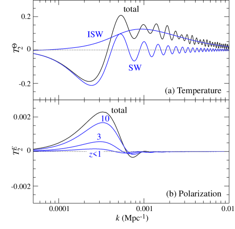
Figure 1: The quadrupole transfer function in the fiducial adiabatic model (see text). The temperature quadrupole receives Sachs-Wolfe (SW) contributions peaking around $k=0.0002$ Mpc^-1 and Integrated Sachs-Wolfe (ISW) contributions peaking around $k=0.001$ Mpc^-1 but extending to $k\sim 0.01$ Mpc^-1. The ISW effect arises from the dark energy dominated regime $z\lesssim 1$. The polarization arises through rescattering of quadrupole anisotropies at $z>1$ and hence reflects the SW contributions. The cross correlation is proportional to the product of the transfer functions.

Let us define the two dimensional CMB transfer functions as the mapping between the power in the initial curvature fluctuations $\zeta_{i}$ in the comoving gauge [see Appendix, Eqn. (69)]

$$\langle\zeta_{i}({\bf k})\zeta_{i}({\bf k}^{\prime})\rangle=(2\pi)^{3}\delta({\bf k}-{\bf k}^{\prime}){2\pi^{2}\over k^{3}}\Delta_{\zeta_{i}}^{2}(k)\,$$ (1)

and the angular space power spectra

$${\ell(\ell+1)C_{\ell}^{XX^{\prime}}\over 2\pi}=\int{dk\over k}T_{\ell}^{X}(k,\eta_{0})T_{\ell}^{X^{\prime}}(k,\eta_{0})\Delta_{\zeta_{i}}^{2}(k)\,,$$ (2)

where $X,X^{\prime}\in\Theta,E$ the temperature fluctuation and $E$-mode polarization respectively.

We employ a comoving gauge Boltzmann hierarchy code Hu and Okamoto (2003) for numerical solutions of the transfer function. These are shown for the temperature and polarization quadrupole in Fig. 1. Here we have chosen fiducial values for the cosmological parameters that are near the maximum likelihood model from WMAP: a dark energy density relative to critical of $\Omega_{Q}=0.73$, non-relativistic matter density $\Omega_{m}h^{2}=0.14$, baryon density $\Omega_{b}h^{2}=0.024$, optical depth to reionization $\tau=0.17$, dark energy equation of state $w_{Q}=p_{Q}/\rho_{Q}=-1$ in a spatially flat universe. The resulting temperature power spectrum is shown in Fig. 2 compared with the WMAP data for a scale invariant spectrum of initial perturbations

$$\Delta_{\zeta_{i}}^{2}=\delta_{\zeta_{i}}^{2}\left({k\over 0.05{\rm Mpc}^{-1}}\right)^{n-1}$$ (3)

where $\delta_{\zeta_{i}}=5.07\times 10^{-5}$ and the tilt $n=1$.

Figure 2: Temperature power spectrum in the fiducial model compared with the data from the first year WMAP release Verde et al. (2003). Bands are 68% and 95% cosmic variance confidence regions (see text).

Notice that the temperature contributions from the SW and ISW effects are comparable in magnitude and well-separated in scale. Hence they add nearly in quadrature in Eqn. (2). In the polarization, the quadrupole comes mainly from the SW effect as can be seen from its dependence on the redshift of reionization or equivalently the cumulative contributions from $z<z_{\rm max}$ (see Fig. 1b). The polarization quadrupole gets nearly no contributions from $z<1$ when the dark energy dominates. These properties are the key to understanding how to construct a model with certain desired properties at low temperature and polarization multipoles.

Since the quadrupoles are dominated by large scale or low-$k$ fluctuations, it is useful to examine the origin of these properties with a low-$k$ approximation to the transfer functions. In this limit, the transfer function is determined by the Newtonian temperature monopole $\Theta$, gravitational potential $\Psi$ and curvature fluctuation $\Phi$ [see Eqn. (71), (72) for the correspondence to the comoving gauge]

$$T_{\ell}^{\Theta}(k,\eta_{0}) = {\sqrt{2\ell(\ell+1)}\over\zeta_{i}}\Big{[}{({\Theta_{*}+\Psi_{*}})j_{\ell}(kD_{*})}$$ (4)

$$+\int_{\eta_{*}}^{\eta_{0}}d\eta(\dot{\Psi}-\dot{\Phi})j_{\ell}(kD)\Big{]}$$

$$\approx -{\sqrt{2\ell(\ell+1)}\over\zeta_{i}}\Big{[}{1\over 5}\zeta_{i}j_{\ell}(kD_{\rm m})$$

$$+2\int_{\eta_{\rm m}}^{\eta_{0}}d\eta\,\dot{\Phi}\,j_{\ell}(kD)\Big{]}\,,$$

where the subscripts denote evaluation at recombination for $``*"$, $``0"$ for the present and “m” for some arbitrary time well after radiation domination but well before dark energy domination and overdots represent derivatives with respect to conformal time $\eta=\int dt/a$. Here we have assumed a spatially flat universe where the comoving distance $D=\eta_{0}-\eta$. Since $\Phi\approx-\Psi$ when the anisotropic stress is negligible [see Eqn. (72)], we loosely refer to either as the gravitational potential.

The two terms in the second line are the SW and ISW effects respectively. This approximation accounts for the small evolution in the gravitational potential between recombination and full matter domination, sometimes called the “early” ISW effect. Since $D_{\rm m}\approx D_{*}$, this effect adds coherently with those at recombination. In the fiducial cosmology, $D_{*}\approx 14$Gpc. Since $j_{\ell}(x)$ peaks at $x\approx\ell+1/2$, the SW contributions peak at $x=5/2$ or $k\sim 0.0002$ Mpc in Fig. 1. The temporal evolution for the potential and quadrupole are shown for this mode in Fig. 3a.

Figure 3: Time evolution of gravitational potential $\Phi$ and quadrupole $T_{2}^{\Theta}$ in the fiducial adiabatic model compared an adiabatic plus isocurvature model with $S_{i}\equiv\delta_{Qi}/\zeta_{i}=-15$ (A&I; see §III). (a) $k=0.0002$ Mpc^-1 SW dominated mode. In the adiabatic model, the decay of the potential at $z\lesssim 1$ has little effect on the quadrupole due to the inefficiency in the transfer represented by $j_{2}$. A much larger change of $\Delta\Phi\sim-\zeta_{i}$ from the isocurvature perturbation can cancel the SW quadrupole. (b) $k=0.001$ Mpc^-1 ISW dominated mode. The adiabatic potential decay transfers efficiently onto the quadrupole moment. The additional isocurvature perturbations decay by dark energy domination and have little effect (see Fig. 4).

The ISW effect arises from the change in the gravitational potential due to the dark energy. In the adiabatic model, the smooth dark energy density accelerates the expansion without enhancing the density perturbations and leads to a decay of the potential at $z\lesssim 1$ (see Fig. 3). Naively, one would suppose that a decay of $\Delta\Phi=-\zeta_{i}/10$ would be sufficient to cancel out the SW effect of $\zeta_{i}/5$. For superhorizon scaled adiabatic fluctuations in a flat universe the conservation of the comoving curvature implies Bardeen (1980)

$$\Delta\Phi\equiv \Phi(k,a=1)-\Phi(k,a_{\rm m})$$

$$\approx \left({2\over 5}-{H_{0}}\int_{a_{\rm m}}^{1}{da^{\prime}\over H}\right)\zeta_{i}\,,$$ (5)

where the approximation assumes $a_{\rm m}\ll 1$ is some epoch near the beginning of matter domination so that contributions near the lower limit of the integral may be ignored. Here $H=a^{-1}da/dt$ is the Hubble parameter. In the fiducial model $\Delta\Phi\approx-0.14\zeta_{i}$. However the distance to $z\lesssim 1$ is much smaller than $D_{*}$ and that degrades the efficiency with which the ISW effect contributes in Eqn. (4). The efficiency factor $j_{2}(kD)$ implies that one requires factor of 10 greater change in the potential (or $\Delta\Phi\sim-\zeta_{i}$) to affect the quadrupole substantially (see Fig. 3). At the peak of the SW effect in $k$, the ISW effect has little effect (see Fig. 1).

Contributions from the ISW effect in the quadrupole actually originate from scales where $kD_{\rm de}\approx 5/2$ where “de” denotes the epoch of dark energy-matter equality. Because the distance changes rapidly with redshift locally, the ISW effect is spread out across over a factor of ten in physical scale with a peak centered near $k=0.001$ Mpc^-1 (see Fig. 1a). At this wavenumber $j_{2}(kD)$ has a peak near $z=1$ corresponding to an efficient transfer of power. Moreover since the decay occurs on the expansion time scale the oscillations in $k$ from $j_{l}(kD)$ in the ISW integrand of Eqn. (4) are washed out in the transfer function. Physically this reflects the cancellation of radial modes as photons travel in and out of decaying gravitational potentials along the line of sight.

To lower the predicted value of the quadrupole, one can alter the fiducial model to lower the SW effect, the ISW effect or both. Since both effects contribute nearly equally, reducing one or the other can at best halve the power. Of course, due to cosmic variance, it is possible that the observed quadrupole results from a lack of angular power in our given realization of the fiducial model. In Fig. 2 we show the 68% and 95% cosmic variance confidence regions assuming that $C_{\ell}^{\Theta\Theta}$ is distributed as a $\chi^{2}$ with $2\ell+1$ degrees of freedom around the fiducial model. However again, a simple lack of power on large physical scales for our last scattering (recombination) surface is not sufficient. Unless our local volume also lacks intermediate scale power as well, a chance occurrence of a low observed quadrupole would result from a chance cancellation of the SW and ISW effects.

The low multipole polarization and cross spectra provides key additional information to discriminate between alternatives. In the large scale limit, it is approximately

$$T_{\ell}^{E}(k,\eta_{0}) =-{3\over 4}\sqrt{(\ell+2)!\over(\ell-2)!}\int_{\eta_{*}}^{\eta_{0}}d\eta\dot{\tau}e^{-\tau}T_{2}^{\Theta}(k,\eta){j_{\ell}(kD)\over(kD)^{2}}\,,$$ (6)

where $\tau$ is the Thomson optical depth as measured from the observer. Consider the transfer function of the polarization quadrupole. Fig. 1 shows that in the fiducial model it is generated before the temperature quadrupole is modified by the ISW effect. Consequently, the transfer function also peaks near the large scales of the SW peak of $k\sim 0.0002$ Mpc^-1. As Eqn. (2) shows this overlap is also the origin of the temperature-polarization cross correlation. In Fig. 7, we show the $EE$ and $\Theta E$ power spectra of the fiducial model.

If the explanation of the observed low quadrupole involves the dark energy, either through a dynamical effect or chance cancellation, one would expect a polarization quadrupole and hence $EE$ power that is not anomalously low compared with the fiducial model. If on the other hand it involves an actual lack of predicted long-wavelength power in the model or by chance, both spectra would be low. Finally, if the explanation involved only the reduction of the ISW effect and no modification of long wavelength power, then the predicted $\Theta E$ cross power spectrum would also remain unchanged.

III Dark Energy Models

The fact that in the fiducial adiabatic model the temperature quadrupole receives comparable contributions from recombination and dark energy domination through the SW and ISW effects raises the possibility that the low quadrupole originates in the dark energy sector. In the Appendix we present a detailed treatment of perturbation theory in general dark energy models which provides the basis for results in this section.

The essential element that defines the ISW effect in the fiducial model is that the dark energy remains smooth out to the horizon scale and hence does not contribute density fluctuations to the gravitational potential. In general there are two ways to alter this conclusion: modify the dynamics of the dark energy so that dark matter fluctuations remain imprinted on the dark energy or modify the initial perturbations in the dark energy sector. Since the dark energy has made a negligible contribution to the net energy density until recently, the latter represents contributions from an isocurvature initial condition. That dark energy isocurvature conditions can help to lower the quadrupole has recently been shown Moroi and Takahashi (2004). Here we present a general discussion on the requirements of such a model.

The first requirement is that an initial dark energy perturbation must survive evolution in the radiation and matter dominated epoch and must remain correlated with the perturbations in the dark matter. The latter condition is required for the dark energy perturbations to cancel the adiabatic ones.

Let us take the dark energy to be a scalar field $Q$ with the canonical kinetic term and a potential $V_{Q}$, i.e. quintessence. We treat the more general case of k-essence in the Appendix. Given that a quintessence field has an effective sound speed $c_{e}=1$ [see Eqn. (58)], coherence well inside the horizon and hence cancellation with the adiabatic ISW effect is not possible. The dark energy isocurvature mechanism then must operate on large scales to cancel the SW effect.

Recall that to achieve a coherent cancellation of the SW effect in the quadrupole one requires either a change of $\Delta\Phi\sim-\zeta_{i}/10$ in the gravitational potential early on when $D\approx D_{*}$ or a larger change $\Delta\Phi\sim-\zeta_{i}$ at $z\lesssim 1$ to compensate for the inefficiency of the transfer of power to the quadrupole. Given that observations require that $w_{Q}\sim-1$ today, the former possibility is excluded unless $w_{Q}$ evolves substantially from its present value.

In a flat universe the comoving curvature evolves only in response to stress fluctuations in the combined or total (“T”) stress energy tensor of the components (see Eqn. 69)

$$\zeta(a,k)= \zeta_{i}(k)-\int_{0}^{a}{da^{\prime}\over a^{\prime}}{\delta p_{T}\over\rho_{T}+p_{T}}$$

$$\approx \zeta_{i}(k)-\int_{a_{\rm m}}^{a}{da^{\prime}\over a^{\prime}}{\delta p_{Q}\over\rho_{m}}\,,$$ (7)

where the approximation assumes $w_{Q}\approx-1$, $a\gg a_{\rm m}$, and the radiation and hence the anisotropic stress is negligible. The generalization of Eqn. (5) for the evolution in the Newtonian potential is [see e.g. Hu and Eisenstein (1999) Eqn. (52)]

$$\Phi(a,k)= \zeta(a,k)-{H\over a}\int_{a_{\rm m}}^{a}{da^{\prime}\over H}[\zeta-{\delta p_{T}\over\rho_{T}+p_{T}}]$$

$$\approx \zeta(a,k)-{H\over a}\int_{a_{\rm m}}^{a}{da^{\prime}\over H}[\zeta-{\delta p_{Q}\over\rho_{m}}]\,.$$ (8)

Thus it requires a substantial pressure fluctuation to make an order unity change to gravitational potential during the dark energy dominated regime

$${\delta p_{Q}\over\rho_{m}}(a=1,k)={\Omega_{Q}\over\Omega_{m}}{\delta p_{Q}\over\rho_{Q}}(1,k)={\cal O}(\zeta_{i})\,.$$ (9)

Note that in the comoving gauge, adiabatic density fluctuations scale as $\delta\sim(k\eta)^{2}\zeta_{i}$ [see Eqn. (76)] and are negligible outside the horizon. Furthermore we shall see below that the order unity coefficient in front of $\zeta_{i}$ is in practice substantially greater than unity.

This requirement severely limits the range of quintessence models which can affect the quadrupole. As shown in the Appendix, aside from transient initial condition effects, an isocurvature perturbation to the quintessence field $\delta Q$ at best remains constant outside the horizon and hence one requires a large initial fluctuation to the quintessence field.

A constant superhorizon quintessence field fluctuation generically occurs if the background field itself is nearly frozen by the Hubble drag so as to only experience a range in the potential where

$$V_{Q}^{\prime}\equiv{dV_{Q}\over dQ}$$ (10)

can be approximated as constant. More specifically, we require that the field not be in the tracking regime or (Steinhardt et al. (1999) see also Appendix)

$$\Gamma\equiv{V_{Q}^{\prime\prime}\over V_{Q}}\left({V_{Q}^{\prime}\over V_{Q}}\right)^{-2}\lesssim 1\,.$$ (11)

To see the consequences for the energy density and pressure, note that aside from a transient decaying mode the Klein-Gordon equation (63) has the solution

$${dQ\over d\ln a}\approx-{2\over 3(3+w_{T})}{V_{Q}^{\prime}\over H^{2}}\,,$$ (12)

where we have assumed an epoch during which $w_{T}=p_{T}/\rho_{T}$ the equation of state of the background is constant. The dark energy density is the sum of the kinetic and potential components

$$\rho_{Q}={1\over 2}\left(H{dQ\over d\ln a}\right)^{2}+V_{Q}\,.$$ (13)

Since $H^{2}\propto\rho_{T}$ decreases with the expansion, if the field is potential energy dominated today ($w_{Q}\sim-1$) then it is potential energy dominated for the past expansion history. The combination of Eqn. (12) and (13) shows that this will be satisfied if the potential satisfies

$${1\over 2}\left(V_{Q}^{\prime}\over V_{Q}\right)^{2}{V_{Q}\over H_{0}^{2}} \lesssim 1\,,$$ (14)

or equivalently with

$$\epsilon_{Q}={1\over 16\pi G}\left({V_{Q}^{\prime}\over V_{Q}}\right)^{2}\,,$$ (15)

and

$$\Omega_{Q}\approx{8\pi GV_{Q}\over 3H_{0}^{2}}\,,$$ (16)

the condition becomes

$$3\Omega_{Q}\epsilon_{Q}\lesssim 1\,.$$ (17)

Moreover since the field only experiences a small range in the potential throughout the whole expansion history, any underlying form of $V_{Q}$ that satisfies these requirements will have the same phenomenology. We find that in the context of the fiducial model $\epsilon_{Q}\lesssim 0.6$ is required for $w_{Q}(a=1)\lesssim-2/3$.

Given potential energy domination, the energy and pressure fluctuations are related to the field fluctuations as

$$\delta\rho_{Q}\equiv\delta_{Q}\rho_{Q}=-\delta p_{Q}=V_{Q}^{\prime}\delta Q$$ (18)

and remain nearly constant during the evolution. The superhorizon evolution of the comoving curvature from Eqn. (7) is given by

$$\zeta(a,k)=\zeta_{i}(k)+{1\over 3}{\delta_{Q}}{\Omega_{Q}\over\Omega_{m}}a^{3}$$ (19)

and hence from Eqn. (8)

$$\Phi(a,k)= \left[1-{H\over a}\int_{a_{\rm m}}^{a}{da^{\prime}\over H}\right]\zeta_{i}$$

$$+\left[1-4{H\over a}\int_{a_{\rm m}}^{a}{da^{\prime}\over H}{a^{\prime}}^{3}\right]{1\over 3}\delta_{Q}{\Omega_{Q}\over\Omega_{m}}$$ (20)

where the two pieces are the adiabatic term and the isocurvature term. The integrals in Eqn. (20) can be expressed in terms of hypergeometric functions. In the fiducial model

$$\Phi(a=1,k)=0.46\zeta_{i}+0.12\delta_{Q}\,.$$ (21)

Combined with the requirement that $\Delta\Phi\approx-\zeta_{i}$ this relation implies that we should set the initial dark energy fluctuations to be $\delta_{Qi}\approx-8\zeta_{i}$ to cancel the quadrupole in the fiducial model.

Figure 4: Isocurvature dark energy density perturbation evolution for a nearly frozen background quintessence field (see text). On superhorizon scales the comoving gauge density perturbation remains frozen at nearly its initial value. On subhorizon scales, the pressure gradients associated with field fluctuations cause the density perturbation to oscillate and decay. Also shown are the dark energy equation of state $w_{Q}=p_{Q}/\rho_{Q}$ and the adiabatic sound speed squared $c_{a}^{2}=\dot{p}_{Q}/\dot{\rho}_{Q}$ (not to be confused with the effective sound speed $c_{e}=1$) which indicate the field is Hubble drag dominated until recently (see Appendix).

While this condition is roughly correct, the scales that are responsible for the quadrupole in the SW effect ($k\sim 0.0002$ Mpc^-1) are on the horizon scale today. Since the quintessence field has a sound horizon equal to the horizon, the fluctuations in these modes will have already begun to decay from their initial values. In Fig. 4 we show the time evolution of the dark energy density perturbation. Because the argument above might appear to require $w_{Q}=-1$ exactly, we have chosen to illustrate the behavior in a model with $w_{Q}(a=1)=-0.94$ and $\epsilon_{Q}=0.18$ with the other parameters equal to their fiducial values. Since $w_{Q}\rightarrow-1$ rapidly with redshift, the change in $D_{*}$ from the fiducial model is only $0.4\%$. As the background evolution is nearly indistinguishable from the true fiducial model, we will employ this choice for the isocurvature analog of the fiducial model.

In practice we have taken a potential $V_{Q}=m_{Q}^{2}Q^{2}/2$ with $m_{Q}=10^{-42}$ GeV and an initial position consistent with $\epsilon_{Q}$ and $dQ/d\ln a=0$ initially. For scales near the peak of the SW effect in the quadrupole the density perturbation has decayed by about a factor of two by $z\sim 1$. Consequently an initial density perturbation of

$$S_{i}\equiv{\delta_{Qi}\over\zeta_{i}}=-15$$ (22)

should be optimal for reducing the SW quadrupole. We call models with this type of fully correlated adiabatic and isocurvature models “A&I” models.

In Fig. 3 we show the effect of this initial condition on the gravitational potential. In this case the change in the gravitational potential $\Delta\Phi\approx-\zeta_{i}$ and one achieves the desired effect of eliminating the SW effect in the quadrupole.

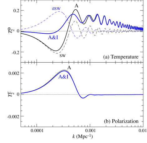
Figure 5: Quadrupole transfer functions in the fiducial adiabatic model (“A”) and a model with additional isocurvature perturbations of $S_{i}=-15$ (“A&I”). The isocurvature ISW effect (iISW) cancel the SW effect for the temperature quadrupole from large scales while leaving the polarization nearly unchanged.

The reduction of the SW quadrupole must not come at the expense of an enhancement in the ISW contributions to the quadrupole. Fortunately, this is a natural consequence of the effective sound speed of the scalar field $c_{e}=1$. Scales near the peak contribution of the adiabatic ISW effect are well within the horizon by dark energy domination. Consequently as can be seen in Fig. 4 any initial isocurvature perturbation in the dark energy will have decayed before dark energy domination. In Fig. 3, we show the evolution of the potential given the initial conditions of Eqn. (22). Note that despite the large initial isocurvature perturbation it has almost no effect on the potential evolution and hence the contributions to the quadrupole.

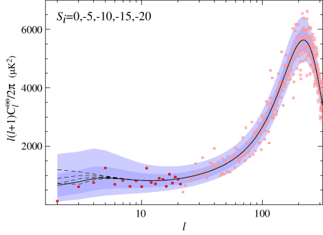
Figure 6: Temperature power spectrum of the A&I model with several choices for the initial isocurvature amplitude compared with the WMAP data. The shaded region corresponds to the 68% and 95% cosmic variance confidence region of the fiducial A&I model with $S_{i}=-15$ (solid line).

In Fig. 5, we show the temperature and polarization transfer functions of the isocurvature model. The isocurvature ISW effect almost perfectly cancels the SW effect on large scales leaving a quadrupole that consists almost solely of the adiabatic ISW effect. Note that the isocurvature conditions leave the polarization essentially unmodified as expected since they only change the potentials at $z\lesssim 2$ in Fig. 3.

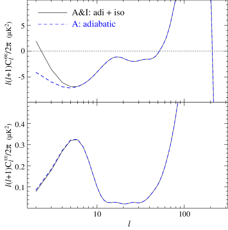
Figure 7: The polarization $EE$ and cross correlation $\Theta E$ spectra for the fiducial adiabatic model compared with the fiducial A&I model of Fig. 6 with $S_{i}=-15$. Although the $EE$ spectrum remains essentially unchanged, the correlation is modified at the low multipoles due to the reduction of the large scale contributions to the quadrupole from the SW effect which are the source of the correlation in the adiabatic model.

In Fig. 6 we show the temperature power spectrum of this model for several choices of $S_{i}$ with all other parameters held fixed. Note that for $S_{i}\approx-15$ the suppression is fairly sharp around the quadrupole in spite of scale invariance in both the adiabatic and isocurvature initial conditions. The polarization auto ($EE$) and cross ($\Theta E$) spectra are shown in Fig. 7. Notice that although the $EE$ spectrum remains nearly unchanged, the $\Theta E$ spectrum has a reduced cross correlation with a sign change at the quadrupole. (Note that our sign convention for $E$ is opposite to CMBFAST.) Because the cross spectrum in the adiabatic case arises from the correlation between the SW quadrupole and the polarization, it is affected by the cancellation of the SW quadrupole as the product of the two transfer functions in Fig. 5 show.

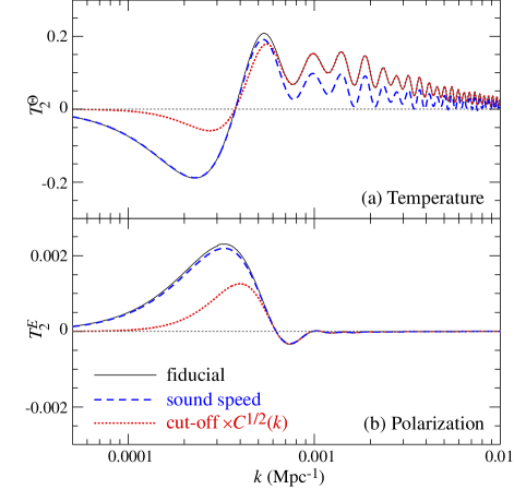
Figure 8: Alternate models for the low quadrupole. The adiabatic ISW effect may be reduced by lowering the effective sound speed of the dark energy, here to $c_{e}=0.03$. The SW effect can be largely eliminated through a cut off factor $C(k)$ in the initial adiabatic power spectrum, here chosen to remove power for $k<k_{\rm cut}=0.0005$ Mpc^-1. Although the latter does not modify the transfer function, we have illustrated its effects by showing $T_{\ell}C^{1/2}(k)$. Note that the cut off affects the polarization whereas the sound speed does not.

It is interesting to compare the isocurvature method of lowering the quadrupole to other possible solutions. A related mechanism involves modifying the sound speed of the dark energy Hu (1998); Dedeo et al. (2003); Erickson et al. (2002); Bean and Dore (2004). Here one retains adiabatic initial conditions but modifies the effective sound speed of the dark energy (see Appendix). The dark energy then contributes density fluctuations between the horizon and the sound horizon and reduces the adiabatic ISW effect by suppressing the decay of the gravitational potential. In Fig. 8, we show the transfer functions for a model with $w_{Q}=-2/3$, $c_{e}=0.03$ with $\Omega_{Q}=0.37$ and $\Omega_{m}h^{2}$ and $\Omega_{b}h^{2}$ held fixed to the fiducial values such that $D_{*}$ and the shape of the peaks remain the same as in the fiducial model. Note that unlike in the isocurvature case, the SW contributions to the quadrupole are unmodified but the adiabatic ISW contributions are reduced. The resulting effect on the temperature power spectrum is shown in Fig. 9. However, like the isocurvature case, the polarization is largely unchanged since the dark energy again only affects low redshifts. A qualitative difference appears in the cross power spectra, which remains unchanged in this case (see Fig. 10).

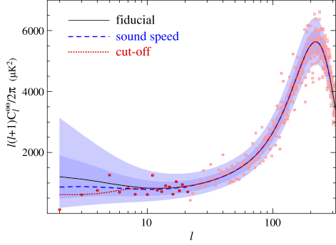
Figure 9: Temperature power spectra of the sound speed and cut off models of Fig. 8. The sound speed model lowers the adiabatic ISW contributions to the quadrupole. The cut off model reduces the SW contributions to the quadrupole.

Finally, the quadrupole can be lowered by removing power on scales associated with the SW effect. Here we take the model Contaldi et al. (2003)

$$\Delta^{2}_{\zeta_{i}}(k)= \Delta^{2}_{\zeta_{i}}(k)|_{\rm fid}C(k)\,,$$

$$C(k)= 1-e^{-(k/k_{\rm cut})^{n_{\rm cut}}}\,,$$ (23)

with $k_{\rm cut}=0.0005$ Mpc^-1 and $n_{\rm cut}=3.35$. The transfer functions for this model are the same as the fiducial model but for illustrative effect we plot them as $T_{\ell}(k)C^{1/2}(k)$ in Fig. 8. Like the isocurvature model, the quadrupole in Fig. 9 is suppressed due to the elimination of the SW quadrupole. Unlike the isocurvature case, both the $EE$ and $\Theta E$ spectra are suppressed since the temperature quadrupoles are also absent during reionization (see Fig. 10).

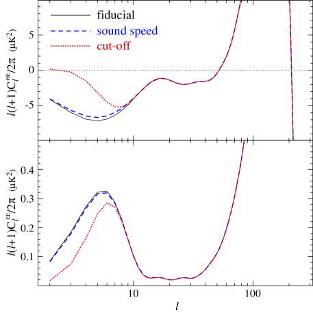
Figure 10: Polarization spectra for the sound speed and cut off models of Fig. 8. The sound speed model changes both spectra negligibly whereas the cut off model suppresses power in both spectra simultaneously.

IV Likelihood Analysis

In this section we check whether the adiabatic plus isocurvature (A&I) model of the previous section is favored by the WMAP data Bennett et al. (2003). For simplicity we will assume a scale invariant spectrum, zero background curvature and zero neutrino mass. Then the maximum likelihood fit with no dark energy perturbations is given in Table 1.

Table 1: Scale Invariant $\Lambda$CDM Model Parameters: WMAP $\Theta\Theta$ $\&$ $\Theta E$ Data.

Parameter	Maximum Likelihood
Matter / Critical Density, $\Omega_{m}$	0.27
Baryon / Critical Density, $\Omega_{b}$	0.046
Hubble Constant, $h$	0.72
Optical Depth, $\tau$	0.17
Initial Amplitude, $\delta_{\zeta_{i}}$	5.07$\times$ $10^{-5}$

When the spectral index is fixed the only parameter with enough freedom to significantly effect the low multipoles is the optical depth, $\tau$.

Keeping the other parameters in Table 1 fixed we vary the magnitude $S_{i}$ of the primordial isocurvature perturbation in dark energy relative to the comoving curvature between $-60<S_{i}<25$ and the optical depth $0<\tau<0.29$ on a $28\times 30$ grid. The amplitude in Table 1 is scaled by $\exp(\tau-0.17)$; recall that the power spectrum is scaled as the square of this quantity [see Eqn. (3)]. This is to take into account the well known degeneracy between $\tau$ and the amplitude. For each grid point the likelihood was evaluated using the software provided by WMAP Hinshaw et al. (2003); Verde et al. (2003) and the resulting two dimensional surface was interpolated. A uniform prior in both parameters was assumed.

The maximum likelihood points are $S_{i}=-15.3$ and $\tau=0.16$ for WMAP $\Theta\Theta$ data only and $S_{i}=-12.1$ and $\tau=0.18$ for WMAP $\Theta\Theta$ and $\Theta E$ data. The $\chi^{2}$ for these parameter values and other models are giving in Table 2. The reduction in $\chi^{2}$ is achieved by only modifying the first few multipoles of the predicted spectrum.

Table 2: Best fit (assuming scale invariance) $\chi^{2}$ and degrees of freedom (DOF) values using WMAP data.

Model	Data	$\chi^{2}$	DOF
Fiducial (Table 1)	$\Theta\Theta$	976	894
$c_{e}=0.03$	$\Theta\Theta$	973	893
Cut-off ($k_{\rm cut}=0.0005$Mpc-1)	$\Theta\Theta$	972	893
Adiabatic & Isocurvature	$\Theta\Theta$	972	893
Fiducial (Table 1)	$\Theta\Theta+\Theta E$	1430	1343
$c_{e}=0.03$	$\Theta\Theta+\Theta E$	1428	1342
Cut-off ($k_{\rm cut}=0.0003$Mpc-1)	$\Theta\Theta+\Theta E$	1428	1342
Adiabatic & Isocurvature	$\Theta\Theta+\Theta E$	1427	1342

Areas enclosing 95% of the probability with and without the $\Theta E$ data are shown in Fig. 11. The area perimeters lie on constant probability contours.

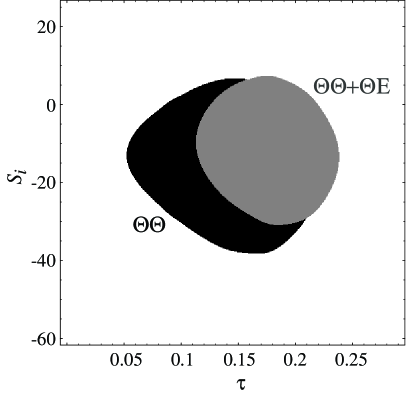
Figure 11: Areas enclosing 95% of the probability for the dark energy isocurvature perturbation ($S_{i}$) and the optical depth ($\tau$). The black area is using only the $\Theta\Theta$ WMAP data and the gray area uses both the $\Theta\Theta$ and $\Theta E$ WMAP data.

As can be seen from Fig. 11, the weight of the probability distribution favors $S_{i}<0$, i.e. an isocurvature density perturbation that is negatively correlated with the comoving curvature perturbation, $\zeta_{i}$. This preference comes from the fact that the lowered temperature quadrupole in such a model better fits the observations. The addition of the $\Theta E$ data reduces the favored magnitude of the isocurvature perturbation $S_{i}$ and slightly increases that of $\tau$ as $\Theta E$ is suppressed in the model but not in the data Dore et al. (2003). Note that the restriction to scale invariant models does not affect the relative improvement that $S_{i}$ makes for a given $\tau$ since across the scales relevant to the first few multipoles any nearly scale invariant model will have the same shape. Allowing the tilt to vary does allow low $\tau$ models if only the $\Theta\Theta$ data is employed but these are eliminated with the inclusion of $\Theta E$ data (c.f. Spergel et al. (2003) and Hansen et al. (2004d)).

One dimensional probability distributions obtained by integrating out $\tau$ are displayed in Fig. 12.

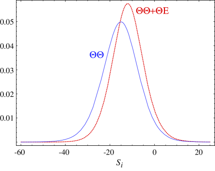
Figure 12: Probability density functions for the dark energy isocurvature perturbation using WMAP $\Theta\Theta$ (solid) and WMAP $\Theta\Theta$ and $\Theta E$ data (dashed).

The mean and 68% confidence regions for $S_{i}$ are $-15.2\pm 8.2$ for WMAP $\Theta\Theta$ data only and $-11.8\pm 7.1$ for WMAP $\Theta\Theta$ and $\Theta E$ data. The probability of $S_{i}>0$ is 0.04 using WMAP $\Theta\Theta$ data only and 0.06 using WMAP $\Theta\Theta$ and $\Theta E$ data. This is in sharp contrast to the estimates of the amount of totally correlated CDM, baryon or neutrino isocurvature perturbation as estimated in Gordon and Lewis (2003); Gordon and Malik (2004) where the probability for a positive isocurvature perturbation was roughly 50%, i.e. the isocurvature perturbation was not significantly different from zero. The reason for this is that correlated non-dark energy isocurvature perturbations have a similar effect on a much larger range of low $\ell$ multipoles as they rely on a simple reduction of the SW effect. The dark energy introduces a scale associated with the current horizon and so the dark energy isocurvature ISW effect can only reduce the SW effect on the large scales associated with the quadrupole.

V Inflationary Context

As we have shown, it is essential that the dark energy isocurvature perturbation is anti-correlated with the adiabatic perturbation so that its ISW effect can coherently cancel the SW effect. Correlated or anti-correlated adiabatic and isocurvature perturbations result when the adiabatic curvature perturbation itself is generated by the isocurvature perturbation Langlois (1999); Gordon et al. (2001). Ref. Moroi and Takahashi (2004) suggested a three field model based on the curvaton mechanism Enqvist and Sloth (2002); Lyth and Wands (2002); Moroi and Takahashi (2001) in order to produce anti-correlated isocurvature dark energy perturbations.

Another way of establishing the anticorrelation is through the variable decay mechanism Dvali et al. (2004); Kofman (2003) where there is a second light scalar field during inflation which determines the decay rate $\Gamma$ of the inflaton. In this method, the resulting comoving curvature perturbation is given by

$$\zeta_{i}=-{1\over 6}{\delta\Gamma\over\Gamma}\,.$$ (24)

If we associate the variable decay field with the quintessence field, $Q$, and take $\Gamma\propto Q$ then $\zeta_{i}=-(1/6)\delta Q/Q$. Then, if we further take the quintessence potential to be $V_{Q}\propto Q^{2}$, we have $\delta_{Q_{i}}=2\delta Q/Q.$ Therefore

$$\delta_{Q_{i}}=-12\zeta_{i}\,,$$ (25)

which was the mean value found in §IV when both WMAP $\Theta\Theta$ and $\Theta E$ data were used.

Unfortunately, a problem with this and other inflationary scenarios arises because of the gravitational waves generated during inflation. Both the scalar field and gravitational waves are nearly massless degrees of freedom during inflation and hence acquire closely related quantum fluctuations. The contribution of the gravitational waves to the $\Theta\Theta$ spectrum for $\ell\gg 1$ is Starobinskii (1985)

$${\ell(\ell+1)\over 2\pi}C_{\ell}^{\Theta\Theta}\Big{|}_{\rm grav}\approx 2\pi G\left(\frac{H_{\rm inf}}{2\pi}\right)^{2}\,,$$ (26)

where $H_{\rm inf}$ is the Hubble parameter during inflation. On the other hand, Eqn. (4) implies that the curvature fluctuations induce a SW effect of

$${\ell(\ell+1)\over 2\pi}C_{\ell}^{\Theta\Theta}\Big{|}_{\rm SW}\approx{1\over 25}\Delta_{\zeta_{i}}^{2}\,.$$ (27)

Now $\Delta_{\zeta_{i}}^{2}$ is related to the inflationary power spectrum of $\delta Q$,

$$\Delta_{\delta Q}^{2}=\left({H_{\rm inf}\over 2\pi}\right)^{2}$$ (28)

through

$$-12\zeta_{i} \approx {\delta_{Qi}}\approx{V_{Q}^{\prime}\over V_{Q}}\delta Q$$ (29)

$$= \sqrt{16\pi G\epsilon_{Q}}\delta Q\,,$$

where $\epsilon_{Q}$ was defined in Eqn. (15). Unlike inflaton curvature fluctuations, these curvature fluctuations are suppressed with a small $\epsilon_{Q}$ because the cancellation condition involves the energy density fluctuation in $Q$. Therefore

$$\frac{\ell(\ell+1)}{2\pi}C_{\ell}\Big{|}_{\rm SW}\approx\frac{G\pi}{225}\epsilon_{Q}\left(\frac{H_{\rm inf}}{2\pi}\right)^{2}.$$ (30)

The predicted ratio of gravitational wave to SW contributions is $r\approx 450/\epsilon_{Q}$.

As discussed in §III, an equation of state today of $w_{Q}\approx-1$ requires a small slow roll parameter for the quintessence ($\epsilon_{Q}\lesssim 0.6$) at the field position today. The current observational limit is about $r<1$ Peiris et al. (2003). Therefore, the isocurvature perturbations in a nearly frozen field model for the quintessence field could not have originated from this inflationary mechanism.

Note that the problem of excess gravitational waves is independent of the precise potential or inflaton decay rate relation as it arises from the phenomenologically required condition Eqn. (25). It applies to any model (including the curvaton model proposed in Ref. Moroi and Takahashi (2004)) for which the field fluctuations $\delta Q$ at dark energy domination are directly associated with the inflationary fluctuations of a light canonical scalar field [Eqn. (28)].

The only way to evade this conclusion is for $\delta Q$ to grow by a factor of 30 or more between horizon crossing during inflation and today. It is not clear how to do this for a canonical scalar field whose perturbations were generated during inflation.

VI Discussion

We have explicated the mechanism by which scale invariant isocurvature perturbations in the dark energy can lead to a sharp suppression of the quadrupole temperature anisotropy Moroi and Takahashi (2004). The Integrated Sachs-Wolfe (ISW) effect in the dark energy dominated epoch can coherently cancel the Sachs-Wolfe (SW) effect from recombination if its energy density fluctuations are set to be strongly anticorrelated with the initial curvature fluctuations. We call these A&I models. Assuming a scale invariant spectrum and flat background, we detect the presence of A&I perturbations at the 95% confidence level.

As is well known Abramo and Finelli (2001); Bartolo et al. (2004); Ferreira and Joyce (1997) (see also Appendix), isocurvature modes in the dark energy rapidly decay for tracking models. Models in which the scalar field and its isocurvature perturbations are essentially frozen Bartolo et al. (2004) due to a shallow potential slope relative to the Hubble parameter are better suited. We have shown that the requirements on such a model comes mainly through the quintessence “slow roll” parameter $\epsilon_{Q}$.

As for the origin of the A&I correlation, we can associate the dark energy with a variable decay rate of the inflaton. We find that the right level of isocurvature perturbations is naturally predicted. Unfortunately, the requirement of a shallow slope of the potential or small $\epsilon_{Q}$ implies too high a level of gravitational waves. For this model to work some mechanism is required for amplifying the field fluctuations by a factor of 30 or more between inflation and dark energy domination.

A&I models should be contrasted with those that introduce a cut off scale to the perturbations. A conceptual problem of the latter class is that it introduces the sharp reduction at the quadrupole “by hand”. In other words, there is a new coincidence problem between the cut-off or topology scale and the horizon today. There is also no significant evidence for features at any other scale (e.g. Mukherjee and Wang (2004); Hannestad (2004)). Phenomenologically, by eliminating the perturbations altogether, the cut off models also eliminate the source of large angle polarization. Thus, the cut-off and A&I models are potentially distinguishable from the polarization autocorrelation (or $EE$) spectrum. On the other hand both models predict a reduced temperature polarization cross correlation.

In principle, these alternatives can also be distinguished by large scale measurements of the density field as a function of redshift and its ISW correlation with the CMB Kesden et al. (2003); Hannestad and Mersini-Houghton (2004); Afshordi (2004); Hu and Scranton (2004), e.g. through high redshift galaxies Crittenden and Turok (1996); Boughn and Crittenden (2004); Fosalba and Gaztanaga (2004); Afshordi et al. (2004) or cosmic shear Hu (2002); Huterer (2002); Song (2004), but measuring the small signals involved will require exquisite control over systematics in the surveys.

Both cut off and A&I models operate by reducing the SW contributions to the quadrupole. Unfortunately, the SW effect only contributes approximately half of the quadrupole in adiabatic models with a cosmological constant. The remaining portion comes from the ISW effect and receives contributions across a wide range of subhorizon scales. Neither A&I nor cut off models can suppress the ISW effect at the quadrupole. In the former, the high sound speed of the dark energy prevents substantial density perturbations on subhorizon scales. In the latter, a cut-off on small enough scales to affect the ISW effect would remove too much small scale power and distort the higher $\ell$ multipoles.

The adiabatic ISW effect can be modified by changing the dynamics of the dark energy by lowering its effective sound speed. Alone it only amounts in a fairly small reduction if the other multipoles are not to be adversely affected. This model is also distinguished from the A&I and cut off models in that it affects neither the auto nor the cross correlation spectra of the polarization. This is because it is the SW quadrupole that is responsible for the polarization and hence its correlation with the temperature.

In combination with an anticorrelated A&I model, a sound speed modification alters the multipole at which the SW effect is canceled. We find that the canonical sound speed $c_{e}=1$ is nearly optimal in producing a sharp suppression at the quadrupole though a slight increase in the sound speed can actually lead to a slightly sharper reduction.

Since the first COBE detection, the low quadrupole temperature anisotropy in the CMB has provided a tantalizing hint that new physics may be hovering on the horizon scale. With upcoming polarization auto and cross correlation data from WMAP, we may soon more than double the information on this intriguing problem. All of the alternatives discussed here have distinct, albeit cosmic variance limited, predictions for these spectra. The predictions are especially distinct at the quadrupole and octopole but it remains to be seen how well these large-angle polarization fluctuations can be separated from galactic foregrounds and instrumental effects.

Acknowledgments: We thank D. Eisenstein and L. Kofman for useful discussions. CG was supported by the KICP under NSF PHY-0114422; WH by the DOE and the Packard Foundation.

Appendix A Dark Energy Perturbations

A.1 Covariant Conservation

Following Bardeen (1980); Kodama and Sasaki (1984), let us define the most general perturbation to the Friedmann Robertson Walker (FRW) metric as

$$g^{00} =-a^{-2}(1-2{A})\,,$$

$$g^{0i} =-a^{-2}{B}^{i}\,,$$

$$g^{ij} =a^{-2}(\gamma^{ij}-2{H}_{L}\gamma^{ij}-2{H}_{T}^{ij})\,,$$ (31)

where $\gamma_{ij}$ is the FRW 3-metric of constant (comoving) curvature $K=H_{0}^{2}(\Omega_{T}-1)$. Likewise let us define the most general stress-energy parameterization of an energy density component $Q$

$$T^{0}_{\hphantom{0}0} =-\rho_{Q},$$

$$T^{0}_{\hphantom{0}i} =q_{Q\,i}\,,$$

$$T^{i}_{\hphantom{i}j} =p_{Q}\delta^{i}_{\hphantom{i}j}+\Pi_{Q}{}^{i}_{\hphantom{i}j}\,,$$ (32)

where $\rho_{Q}$ is the energy density, $q_{Q\,i}$ is the momentum density, $p_{Q}$ is the pressure or isotropic stress and $\Pi_{Q}{}^{i}_{\hphantom{i}j}$is the anisotropic stress of $Q$. The anisotropic stress is defined as the trace free portion of the stress such that $\Pi_{Q}{}^{i}_{\hphantom{i}i}$=0. If $Q$ is to dominate the expansion at any time then $q_{Q}$ and $\Pi_{Q}$ must vanish in the background due to isotropy.

If $Q$ is non-interacting or “dark” then this stress energy tensor is covariantly conserved. Conservation then leads to general equations of motion for the stress-energy components. Retaining terms linear in the metric fluctuations where they combine with stress energy components $(\rho_{Q},p_{Q})$ in the background, we can reduce $\nabla^{\nu}T^{\mu}_{\hphantom{0}\nu}=0$ to

$$\left[{d\over d\eta}+3{\dot{a}\over a}\right]\rho_{Q}= -3{\dot{a}\over a}p_{Q}-\nabla_{i}q^{i}_{Q}$$

$$-(\rho_{Q}+p_{Q})(\nabla_{i}B^{i}+3\dot{H}_{L})\,,$$

$$\left[{d\over d\eta}+4{\dot{a}\over a}\right]q_{Q\,i}= -\nabla_{i}p_{Q}-\nabla_{j}\Pi_{Q}{}^{j}_{\hphantom{j}i}$$

$$-(\rho_{Q}+p_{Q})\nabla_{i}A\,.$$ (33)

The conservation equations represent a general but incomplete description of the dark energy as they leave the spatial stresses $p_{Q}$ and $\Pi_{Q}$ unspecified.

A.2 Equation of State

The isotropic stresses may be rewritten in terms of an equation of state

$$p_{Q}(\eta,x_{i})=w_{Q}(\eta,x_{i})\rho_{Q}(\eta,x_{i})\,,$$ (34)

where $w_{Q}$ is in general a function of position and time.

For the scalar degrees of freedom it is useful to recast Eqn. (33) in terms of an expansion of the fluctuations into scalar harmonic modes defined by the complete set of eigenfuctions $Y$ of the Laplace operator

$$\nabla^{2}Y=-k^{2}Y\,.$$ (35)

The spatial fluctuations in each mode are given by four mode amplitudes ${\delta_{Q},\delta w_{Q},u_{Q},\pi_{Q}}$ as

$${\delta\rho_{Q}}\equiv \delta_{Q}Y\rho_{Q}\,,$$

$${\delta p_{Q}}\equiv (w_{Q}\delta_{Q}+\delta w_{Q})Y\rho_{Q}\,,$$

$${q_{Q\,i}}\equiv u_{Q}(-k^{-1}\nabla_{i}Y)\rho_{Q}\,,$$

$${\Pi_{Q}{}^{i}_{\hphantom{i}j}}\equiv \pi_{Q}(k^{-2}\nabla^{i}\nabla_{j}Y+{1\over 3}\delta^{i}_{\hphantom{i}j}Y)p_{Q}\,.$$ (36)

Note that for a spatially flat metric $Y=e^{i{\bf k}\cdot{\bf x}}$ and the mode amplitudes are the Fourier coefficients of the fields. In the literature (e.g. Bardeen (1980)), one often defines instead a quantity $V_{Q}$, related to the bulk velocity or energy flux, such that $u_{Q}=(1+w_{Q})(V_{Q}-B)$. In Eqn. (36) and throughout the remainder of this section $\rho_{Q}$, $p_{Q}$, and $w_{Q}=p_{Q}/\rho_{Q}$ are to be reinterpreted as the average or background quantities and depend only on time. Hereafter we will typically omit the spatial harmonics $Y$ by assuming a harmonic space representation of the perturbations.

The conservation equations then become

$$\dot{\delta}_{Q}= -3{\dot{a}\over a}\delta w_{Q}-ku_{Q}-(1+w_{Q})(kB+3\dot{H}_{L})\,,$$

$$\dot{u}_{Q}= {\dot{a}\over a}(3w_{Q}-1)u_{Q}+k(w_{Q}\delta_{Q}+\delta w_{Q})$$

$$-{2\over 3}w_{Q}(1-3K/k^{2})k\pi_{Q}+(1+w_{Q})kA\,,$$ (37)

where we have used the conservation of energy relation in the background [see Eqn. (33)]

$$\dot{\rho}_{Q}=-3{\dot{a}\over a}(1+w_{Q})\rho_{Q}\,.$$ (38)

Here we have followed the same convention for the harmonic representation of the metric fluctuations, e.g. $A(\eta,x_{i})=A(\eta,k)Y$.

The quantity $\delta w_{Q}$ represents spatial fluctuations in the equation of state and specifies the pressure fluctuation as

$$\delta p_{Q}=(w_{Q}\delta_{Q}+\delta w_{Q})\rho_{Q}\,.$$ (39)

Equation of state fluctuations can arise from intrinsic internal degrees of freedom in the dark energy or from temporal variations in the background equation of state through a general coordinate or gauge transformation.

The gauge transformation is defined as a perturbation in the temporal and spatial coordinates of $x^{\mu}=\tilde{x}^{\mu}+(T,LY^{i})$ with respect to the background under which Bardeen (1980)

$$A =\tilde{A}-\dot{T}-{\dot{a}\over a}T\,,$$

$$B =\tilde{B}+\dot{L}+kT\,,$$

$$H_{L} =\tilde{H}_{L}-{k\over 3}L-{\dot{a}\over a}T\,,$$

$$H_{T} =\tilde{H}_{T}+kL\,,$$ (40)

for the metric and

$${\delta\rho_{Q}} ={\delta\tilde{\rho}}_{Q}-\dot{\rho}_{Q}T,$$

$${\delta p_{Q}} ={\delta\tilde{p}}_{Q}-\dot{p}_{Q}T,$$

$$u_{Q} =\tilde{u}_{Q}-k(1+w_{Q})T\,,$$ (41)

for the dark energy variables.

Starting from the uniform density gauge where there is no dark energy density fluctuation $\delta\tilde{\rho}_{Q}=0$, there arises a contribution to the pressure fluctuation under the gauge transformation [Eqn. (41)] of

$${\delta p}_{Q}-\delta\tilde{p}_{Q}={\delta\rho_{Q}}c_{a}^{2}\,,$$ (42)

where the adiabatic sound speed is

$$c_{a}^{2}= {\dot{p}_{Q}\over\dot{\rho}_{Q}}={dp_{Q}/d\ln a\over d\rho_{Q}/d\ln a}$$

$$= w_{Q}-{1\over 3}{d\ln(1+w_{Q})\over d\ln a}\,.$$ (43)

If in the uniform density gauge the pressure fluctuation also vanishes ($\delta\tilde{p}_{Q}=0$), the dark energy only has adiabatic pressure fluctuations and from Eqns. (39) and (42)

$$\delta w_{Q\,\rm adi}= (c_{a}^{2}-w_{Q})\delta_{Q}\,.$$ (44)

In this case, the pressure fluctuation and gravitational terms in the momentum conservation equation (37) become

$$kc_{a}^{2}\delta_{Q}+(1+w_{Q})kA\,.$$ (45)

If the dark energy accelerates the expansion $w_{Q}<-1/3$. If $w_{Q}$ is also slowly varying, the adiabatic sound speed is imaginary: $c_{a}^{2}\sim w_{Q}<0$. In the small scale Newtonian approximation (and gauge), the Poisson equation gives $A\sim-\delta_{Q}/(k\eta)^{2}$ during the dark energy dominated epoch. Hence for $c_{a}^{2}<0$ pressure gradients would enhance potential gradients in generating momentum density and the dark energy would collapse faster than the dark matter. Thus for gravitational instability in the dark energy to be stabilized by pressure gradients a source of non-adiabatic pressure fluctuations is required. These can be supplied by internal degrees of freedom in the dark energy.

Following Hu (1998), the role of the background equation of state parameter as a closure relation between the pressure and density can be generalized for an inhomogeneous dark energy component. If one requires that the pressure fluctuation is linear in the energy and momentum density fluctuations, general covariance [or gauge invariance for linear fluctuations, see Eqn. (41)] requires that

$$\delta w_{Q}|_{\rm non-adi}\propto\delta_{Q}+3{\dot{a}\over a}{u_{Q}\over k}\,.$$ (46)

We choose to specify the proportionality through an effective sound speed such that the full equation of state fluctuation is given as

$$\delta w_{Q}= (c_{a}^{2}-w_{Q})\delta_{Q}+(c_{e}^{2}-c_{a}^{2})\left(\delta_{Q}+3{\dot{a}\over a}{u_{Q}\over k}\right)\,.$$ (47)

Note that $c_{e}^{2}=c_{a}^{2}$ for adiabatic pressure fluctuations. The quantity $c_{e}^{2}$ may in principle be a function of time and $k$.

With this ansatz for $\delta w_{Q}$, the covariant conservation equations (37) become

$$\dot{\delta}_{Q}= -3{\dot{a}\over a}(c_{e}^{2}-w_{Q})\delta_{Q}-9\left({\dot{a}\over a}\right)^{2}(c_{e}^{2}-c_{a}^{2}){u_{Q}\over k}$$

$$-ku_{Q}-(1+w_{Q})(kB+3\dot{H}_{L})\,,$$

$$\dot{u}_{Q}= {\dot{a}\over a}[3(w_{Q}+c_{e}^{2}-c_{a}^{2})-1]u_{Q}+kc_{e}^{2}\delta_{Q}$$

$$-{2\over 3}w_{Q}(1-3K/k^{2})k\pi_{Q}+(1+w_{Q})kA\,.$$ (48)

Note that unlike in Eqn. (45), it is $c_{e}^{2}$ and not $c_{a}^{2}$ that is the coefficient for $\delta_{Q}$ in the momentum conservation equation; hence $c_{e}^{2}$ controls the stability of density fluctuations. More formally in the zero momentum gauge or rest frame of the dark energy where $u_{Q}=0$, Eqns. (39) and (47) imply

$$\delta w_{Q\,\rm rest}=(c_{e}^{2}-w_{Q})\delta_{Q\rm rest}\,,$$

$$\delta p_{Q\,\rm rest}=c_{e}^{2}\delta\rho_{Q\rm rest}\,,$$ (49)

so that $c_{e}^{2}$ is the sound speed in the rest frame. This property is useful in the calculation of $c_{e}^{2}$ for a given dark energy model.

Likewise, a closure relation between the anisotropic stress $\pi_{Q}$ and the energy and momentum density can also be supplied through a generalized equation of state Hu (1998). However unlike the non-adiabatic stress, a non-vanishing value is not required for stability by $w_{Q}<-1/3$. We shall see now that for scalar field dark energy candidates it in fact does vanish in linear theory.

A.3 Quintessence and k-Essence Fields

The stress-energy tensor for a scalar field $Q$ with a Lagrangian $F(X,Q)$ is Garriga and Mukhanov (1999)

$$T^{\mu}_{\hphantom{0}\nu}={\partial F\over\partial X}\nabla^{\mu}Q\nabla_{\nu}Q+F\delta^{\mu}_{\hphantom{i}\nu}\,,$$ (50)

where the kinetic term

$$X=-{1\over 2}\nabla^{\mu}Q\nabla_{\mu}Q\,.$$ (51)

For the case of a canonical kinetic energy term

$$F(X,Q)=X-V_{Q}\,,$$ (52)

where $V_{Q}(Q)$ is the scalar field potential. $Q$ is then called the quintessence field. For the case $F(X,Q)=-X-V_{Q}$, the dark energy is called a phantom field (e.g. Caldwell (2002)) and for a more general modification of the kinetic term, a k-essence field Armendariz-Picon et al. (2000).

Matching terms between Eqn. (32) and (50), and dropping contributions that are second order in the spatial gradients of the field

$$\rho_{Q} =2{\partial F\over\partial X}X-F\,,$$

$$p_{Q} =F\,,$$

$$q_{Q\,i} =-{\partial F\over\partial X}a^{-2}\dot{Q}\nabla_{i}Q\,,$$

$${\Pi_{Q}}{}^{i}_{\hphantom{i}j} =0\,.$$ (53)

In particular the density and pressure fluctuations become

$$\delta\rho_{Q}= (2{\partial^{2}F\over\partial X^{2}}X+{\partial F\over\partial X})\delta X+\left(2{\partial^{2}F\over\partial Q\partial X}X-{\partial F\over\partial Q}\right)\delta Q\,,$$

$$\delta p_{Q}= {\partial F\over\partial X}\delta X+{\partial F\over\partial Q}\delta Q\,,$$ (54)

where

$$\delta X=a^{-2}(\dot{Q}\dot{\delta Q}-A\dot{Q}^{2})\,.$$ (55)

Note that under a gauge transformation $Q$ transforms as a scalar

$${\delta Q} ={\delta\tilde{Q}}-\dot{Q}T\,,$$ (56)

and

$$\rho_{Q}u_{Q}={\partial F\over\partial X}a^{-2}\dot{Q}k\delta Q\,.$$ (57)

Hence the uniform field gauge where $\delta Q=0$ coincides with the rest gauge $u_{Q}=0$. Since this is the gauge in which $c_{e}^{2}=\delta p_{Q}/\delta\rho_{Q}$, the effective sound speed of a scalar field is Garriga and Mukhanov (1999),

$$c_{e}^{2}={\partial F/\partial X\over 2(\partial^{2}F/\partial X^{2})X+(\partial F/\partial X)}\,.$$ (58)

For a scalar field with the canonical kinetic term in Eqn. (52), $c_{e}^{2}=1$. More generally, to achieve a constant $c_{e}^{2}$ one requires

$${\partial F\over\partial X}=\left({X\over V_{K}}\right)^{1-c_{e}^{2}\over 2c_{e}^{2}}\,,$$ (59)

where $V_{K}$ is a constant with dimensions of energy density. If for simplicity one further assumes that the kinetic and potential terms are additive $\partial F/\partial Q=-{\partial V_{Q}/\partial Q}$ and

$$F={2c_{e}^{2}\over 1+c_{e}^{2}}\left({X\over V_{k}}\right)^{1+c_{e}^{2}\over 2c_{e}^{2}}V_{k}-V_{Q}\,.$$ (60)

The effective sound speed of Eqn. (58) along with $w_{Q}$ in the background closes the evolution equations Eqn. (48) once the metric fluctuations are specified by the Einstein equations (see §A.5). The evolution of dark energy density perturbations is then completely defined by a choice of initial conditions for $\delta_{Q}$ and $u_{Q}$.

A.4 Background Evolution

To obtain the background evolution of the dark energy, one begins with the energy density conservation equation (38) in terms of the field variables

$$\ddot{Q}+(3c_{e}^{2}-1){\dot{a}\over a}\dot{Q}+c_{e}^{2}a^{2}\left({\partial F\over\partial X}\right)^{-1}{\partial\rho_{Q}\over\partial Q}=0$$ (61)

or

$${d^{2}Q\over d\ln a^{2}}+{3\over 2}(2c_{e}^{2}-1-w_{T}){dQ\over d\ln a}+{c_{e}^{2}\over H^{2}}\left({\partial F\over\partial X}\right)^{-1}{\partial\rho_{Q}\over\partial Q}=0\,.$$ (62)

For the canonical kinetic term,

$${d^{2}Q\over d\ln a^{2}}+{3\over 2}(1-w_{T}){dQ\over d\ln a}+{{1\over H^{2}}{dV_{Q}\over dQ}}=0\,,$$ (63)

where $w_{T}=p_{T}/\rho_{T}$ is the equation of state for the sum of all components. Note that $w_{T}$ depends on $Q$ and hence in practice it is more convenient to solve a set of coupled first order differential equations in $Q$ and $HdQ/d\ln a=\sqrt{2X}$. Likewise, since $1+w_{Q}$ appears in the evolution equations, one calculates this quantity directly as

$$1+w_{Q}={2(\partial F/\partial X)X\over 2(\partial F/\partial X)X-F}\,.$$ (64)

Combined with Eqn. (59), this relation implies that if the field is potential energy dominated $w_{Q}\rightarrow-1$ and if it is kinetic energy dominated $w_{Q}\rightarrow c_{e}^{2}$.

With equation (62), the expression for the adiabatic sound speed becomes

$$c_{a}^{2}=c_{e}^{2}+{c_{e}^{2}\partial\rho_{Q}/\partial Q-\partial F/\partial Q\over 3H^{2}(\partial F/\partial X)({dQ/d\ln a})}\,.$$ (65)

The adiabatic sound speed takes on a specific form in the case where the Hubble drag inhibits the motion of the field. In this case $\partial\rho_{Q}/\partial Q$ is nearly constant. If $w_{T}$ is constant, $dQ/d\ln a$ reaches a “terminal velocity” that is independent of the initial conditions and scales with $H$. Utilizing the constant effective sound speed form for $F$ in equation (60), the equation of motion (62) can be written in the form of the Bernoulli equation and the adiabatic sound speed becomes

$$c_{a}^{2}=c_{e}^{2}-{1\over 2}(c_{e}^{2}+1)(3+w_{T})\,.$$ (66)

For the case of a canonical kinetic term $c_{a}^{2}=-2-w_{T}$ Bartolo et al. (2004) (see also Fig. 4).

On the other hand, if the Hubble drag is negligible

$${dQ\over d\ln a}\propto a^{-3(2c_{e}^{2}-1-w_{T})/2}\,,$$ (67)

and assuming kinetic energy domination $w_{Q}=c_{a}^{2}=c_{e}^{2}$.

A.5 Initial Conditions and Evolution

We numerically solve the dark energy evolution equations in comoving gauge where the total momentum density vanishes

$$\rho_{T}u_{T}\equiv\sum_{i}\rho_{i}u_{i}=0\,.$$ (68)

Here $i$ runs over all species of energy density. We define the total density and pressure fluctuation similarly. The auxiliary condition $H_{T}=0$ completely fixes the coordinate freedom. We call the remaining metric degrees of freedom $\zeta\equiv H_{L}$, $\xi\equiv A$ and $V_{T}\equiv B$, where $V_{T}$ also has the interpretation of the total momentum weighted velocity [see Bardeen (1980) and the discussion below Eqn. (36)]. The Einstein equations become

$$\dot{\zeta}+{K\over k}V_{T}= {\dot{a}\over a}\xi$$

$$= \dot{a\over a}{1\over\rho_{T}+p_{T}}\left[-\delta p_{T}+{2\over 3}\left(1-{3K\over k^{2}}\right)p_{T}\pi_{T}\right]\,,$$

$$V_{T}= (\Phi-\zeta)k\left({\dot{a}\over a}\right)^{-1}$$ (69)

where recall $K$ is the background spatial curvature. The continuity equation for the total density perturbation completes the basic equations

$$\dot{\delta}_{T}=-3{\dot{a}\over a}\delta w_{T}-(1+w_{T})(kV_{T}+3\dot{\zeta})\,,$$ (70)

as the momentum conservation equation was used to relate $\xi$ to the stresses in Eqn. (69). In that equation

$$(k^{2}-3K)\Phi=4\pi Ga^{2}\rho_{T}\delta_{T}$$ (71)

and is equal to the curvature fluctuation in the Newtonian or longitudinal gauge $\Phi\equiv H_{L}|_{\rm Newt}$. For reference, the Newtonian potential $\Psi\equiv A|_{\rm Newt}$ employed in §II is

$$\Psi=-\Phi-8\pi Ga^{2}p_{T}\pi_{T}/k^{2}\,,$$ (72)

and the total velocity obeys an auxiliary relation

$$\dot{V}_{T}+{\dot{a}\over a}V_{T}=-k(\xi-\Psi)$$ (73)

that is useful for checking numerical solutions.

Equation (69) implies that the curvature fluctuation $\zeta$ changes only in response to stress fluctuations. As in the discussion of dark energy perturbations above, the evolution equations are closed through an assumption for the stress perturbations. In practice, for numerical solutions that extend to subhorizon scales, we replace Eqn. (70) with the conservation equations for the individual energy density species to implicitly solve for $\delta w_{T}$.

For the initial conditions, assuming nearly adiabatic stresses

$$\left|\delta p_{T}-{\dot{p}_{T}\over\dot{\rho}_{T}}\delta\rho_{T}\right|\ll|\delta p_{T}|$$ (74)

and a closure relation for the anisotropic stress of the neutrinos which comes from the Boltzmann equation [e.g. Hu (1998) Eqn. (12)]

$$\pi_{\nu}={4\over 5}k\eta V_{T}\,,$$ (75)

we obtain the solution to the evolution equations in the radiation dominated regime

$$\delta_{T}= {4\over 9}{1+3\alpha_{\nu}\over 1+2\alpha_{\nu}}(1-3{K\over k^{2}})(k\eta)^{2}\zeta_{i}\,,$$

$$V_{T}= -{1\over 3}{1\over 1+2\alpha_{\nu}}(k\eta)\zeta_{i}\,,$$ (76)

where $\alpha_{\nu}=2\rho_{\nu}/15\rho_{r}$ accounts for the anisotropic stress of the neutrinos

$$\pi_{T}= {\rho_{\nu}\over\rho_{r}}\pi_{\nu}$$

$$= -{2\alpha_{\nu}\over 1+2\alpha_{\nu}}(k\eta)^{2}\zeta_{i}\,.$$ (77)

Here $\rho_{r}=\rho_{\gamma}+\rho_{\nu}$, the total radiation density and we have kept only leading order terms in power of $k\eta$. Given that the stress perturbation $\delta p_{T}/(\rho_{T}+p_{T})={\cal O}[(k\eta)^{2}]\zeta_{i}$, Eqn. (69) shows that the curvature perturbation is nearly constant for superhorizon adiabatic stresses $\zeta(k,\eta_{i})=\zeta_{i}(k)$ Bardeen (1980).

The dark energy perturbations associated with the curvature fluctuation can then be related to the total density perturbation by substituting these relations back into the Einstein equations (69) for $\dot{\zeta}$ and $\xi$ and employing them in the conservation equations (48). The result is

$$\delta_{Q} =A_{\delta}(1+w_{Q})\delta_{T}\,,$$

$$u_{Q} =A_{u}(1+w_{Q})(k\eta){\delta_{T}}\,,$$ (78)

where assuming a radiation dominated initial condition

$$A_{u} ={3c_{e}^{2}+(1+6\alpha_{\nu})(3w_{Q}-2)\over 4(1+3\alpha_{\nu})[8+3c_{e}^{2}(2-3c_{a}^{2}+3w_{Q})-12w_{Q}]}\,,$$

$$A_{\delta} ={3\over 4}{1-6(c_{e}^{2}-c_{a}^{2})A_{u}\over 1-3(w_{Q}-c_{e}^{2})/2}\,.$$ (79)

We have here assumed that $w_{Q}$ and $c_{a}^{2}$ are nearly constant compared with the expansion time but have allowed $(1+w_{Q})$ to vary as appropriate for a scalar field under the Hubble drag by factoring this quantity out of Eqn. (78).

The curvature initial conditions for the dark energy take on this rather intricate form involving $A_{u}$ in the relation for $A_{\delta}$ since the internal non-adiabatic stress of the dark energy cannot be neglected even though its contribution to the total non-adiabatic stress in Eqn. (74) can be ignored. In general, the curvature mode always carries non-adiabatic stresses beyond the leading order in $(k\eta)$ and $\rho_{i}/\rho_{r}$ where $i\neq\gamma,\nu$. Formally these vanish if the initial conditions are taken to $\eta_{i}\rightarrow 0$.

Deviations in the initial conditions for the dark energy from these relations represents an isocurvature mode since the dark energy is assumed to carry a negligible fraction of the net energy density at the initial conditions so that the radiation density fluctuation $\delta_{r}=\delta_{T}$. If we also assume that the relative deviations are large $\delta_{Q}(\eta_{i},k)\gg(1+w_{Q})\delta_{T}(\eta_{i},k)$ then the dark energy-radiation entropy fluctuation

$$(1+w_{Q})S_{Qr}\equiv \delta_{Q}-{1+w_{Q}\over 1+w_{r}}\delta_{r}\,,$$

$$\approx \delta_{Q}\,,$$ (80)

which corresponds to the usual definition of the isocurvature mode as being generated by $S_{Qr}$. The distinction here is that the adiabatic mode has $S_{Qr}={\cal O}(\delta_{T})\neq 0$ due to the intrinsic entropy of $Q$ and evolution of $w_{Q}$.

Neglecting the metric fluctuations generated by the dark energy fluctuations, we find that the the evolution equations (48) are solved by a linear combination of the adiabatic mode and

$$\delta_{Q} =I_{\delta}(k\eta)^{p}\,,$$

$$u_{Q} =I_{u}(k\eta)^{p+1}\,,$$ (81)

where

$${I_{\delta}\over I_{u}}= \left[p+{3(1+w_{T}+2c_{a}^{2}-2c_{e}^{2}-2w_{Q})\over 1+3w_{T}}\right]c_{e}^{-2}$$

and $p$ solves the equation

$$\left[p+{6\over 1+3w_{T}}(c_{e}^{2}-w_{Q})\right]{I_{\delta}\over I_{u}}=-9\left({2\over 1+3w_{T}}\right)^{2}(c_{e}^{2}-c_{a}^{2})\,.$$ (83)

For initial conditions in the radiation dominated era, the solutions to this quadratic equation are

$$p={-1-{3\over 2}c_{a}^{2}}+3w_{Q}\pm\sqrt{(1+3c_{a}^{2}/2)^{2}-6c_{e}^{2}}\,.$$ (84)

These solutions in fact apply for essentially all gauges until the epoch of dark energy domination. The only exceptions are those that place explicit conditions on the dark energy fluctuations such as $\delta_{Q}=0$ or $u_{Q}=0$.

It is instructive to consider the two limiting cases of Hubble drag domination and negligible Hubble drag or kinetic energy domination in Eqn. (66). In the former case,

$$p=0,\quad{3\over{1+3w_{T}}}(-2+c_{e}^{2}+c_{e}^{2}w_{T})\,.$$ (85)

In terms of the field variables, the constant mode corresponds to an initial condition where $\delta X=0$, i.e. the kinetic energy terms in Eqn. (54) for the density perturbation vanish. Therefore the potential energy fluctuation remains constant. Note that in spite of this the momentum density does not vanish. The second mode corresponds to an initial conditions with comparable kinetic and potential energy ($\delta Q$ terms) in the perturbation. An arbitrary initial condition can be decomposed into a superposition of the modes. Note that the second mode is decaying for $c_{e}^{2}<2/(1+w_{T})$ and growing for $c_{e}^{2}>2/(1+w_{T})$. For a canonical kinetic term, this is a decaying mode for all $w_{T}<1$. Nonetheless, if $2>c_{e}^{2}>3/2$ a small initial density or field fluctuation will be amplified during radiation domination and freeze in during matter domination even though the background field is potential energy dominated during the whole expansion history $w_{Q}\approx-1$.

The existence of this mode could potentially allow a solution to the gravitational wave problem of §V by amplifying the field fluctuations from their initial conditions. However the amount of amplification is dependent on the initial ratio of kinetic to potential energy in the fluctuation. It also depends on the ratio in the background since the fractional fluctuation in the kinetic energy density (as opposed to the total energy density) must also remain small for the mode analysis to remain valid. Finding an explicit model that satisfies these conditions is beyond the scope of this work.

In the opposite regime of kinetic energy domination, the two solutions become

$$p=0,\quad{{3(2c_{e}^{2}-1-w_{T})\over 1+3w_{T}}}\,.$$ (86)

The $p=0$ solution corresponds to a kinetic energy dominated perturbation where $\delta X$ scales with $X$. The other solution corresponds to a pure velocity isocurvature mode where $u_{Q}/(k\eta)\gg\delta_{Q}\approx 0$. Note that $u_{Q}$ grows if $c_{e}^{2}>1/3$ as is the case for the canonical kinetic term. In the field representation, this mode represents a case where the density perturbation is dominated by the potential energy and hence negligible in the kinetic energy dominated regime. The field fluctuation $\delta Q$ then remains constant but the momentum density $u_{Q}$ in Eqn. (57) grows due to the redshifting of $\rho_{Q}$ in the background. If the field later exits from kinetic energy domination, the field fluctuation then becomes an energy density fluctuation.

Finally, there is the well-studied tracking regime where $1+w_{Q}\propto 1+w_{T}$. Then $1+w_{Q}$ is approximately constant and Eqn. (43) gives $c_{a}^{2}\approx w_{Q}$. The two solutions become

$$p= -{3\over 2(1+3w_{T})}\Big{(}1-2w_{Q}+w_{T}$$

$$\pm\sqrt{(1+2w_{Q}+w_{T})^{2}-8c_{e}^{2}(1+w_{T})}\Big{)}\,.$$ (87)

The index $p$ is maximized by maximizing $w_{Q}$. The maximum $w_{Q}=c_{e}^{2}$ for a kinetic energy dominated field and hence the fastest growing modes are given by Eqn. (86). By further requiring the tracker condition $w_{Q}<(1+w_{T})/2$ Steinhardt et al. (1999), we see that Re$(p)<0$ and there are again no growing modes. The field fluctuations then “track” and lose their dependence on the initial isocurvature perturbation as is well known. Note that for the canonical kinetic term in the tracking regime, the proportionality is Steinhardt et al. (1999)

$$1+w_{Q}\approx{1+w_{T}\over 2\Gamma-1}$$ (88)

where $\Gamma$ was defined in Eqn. (11). The perfect tracker is attained at the limiting case of $1+w_{Q}=1+w_{T}$ or $\Gamma=1$ which is acheived for an purely exponential potential $V_{Q}\propto e^{-CQ}$ where $C$ is constant Ferreira and Joyce (1997). Here the dark energy remains a constant fraction of the total energy density.

References

- Bennett et al. (2003) C. L. Bennett et al., Astrophys. J. Suppl. 148, 1 (2003), eprint astro-ph/0302207.
- Spergel et al. (2003) D. N. Spergel et al., Astrophys. J. Suppl. 148, 175 (2003), eprint astro-ph/0302209.
- Peiris et al. (2003) H. V. Peiris et al., Astrophys. J. Suppl. 148, 213 (2003), eprint astro-ph/0302225.
- Efstathiou (2003) G. Efstathiou, Mon. Not. R. Astron. Soc. 346, L26 (2003), eprint astro-ph/0306431.
- Efstathiou (2004) G. Efstathiou, Mon. Not. R. Astron. Soc. 348, 885 (2004), eprint astro-ph/0310207.
- Tegmark et al. (2003) M. Tegmark, A. de Oliveira-Costa, and A. Hamilton, Phys. Rev. D68, 123523 (2003), eprint astro-ph/0302496.
- Slosar et al. (2004) A. Slosar, U. Seljak, and A. Makarov (2004), eprint astro-ph/0403073.
- Slosar and Seljak (2004) A. Slosar and U. Seljak, Phys. Rev. D submitted (2004), eprint astro-ph/0404567.
- de Oliveira-Costa et al. (2004) A. de Oliveira-Costa, M. Tegmark, M. Zaldarriaga, and A. Hamilton, Phys. Rev. D 69, 063516 (2004), eprint astro-ph/0307282.
- Schwarz et al. (2004) D. J. Schwarz, G. D. Starkman, D. Huterer, and C. J. Copi (2004), eprint astro-ph/0403353.
- Bielewicz et al. (2004) P. Bielewicz, K. M. Gorski, and A. J. Banday (2004), eprint astro-ph/0405007.
- Eriksen et al. (2004a) H. K. Eriksen, A. J. Banday, K. M. Gorski, and P. B. Lilje (2004a), eprint astro-ph/0403098.
- Eriksen et al. (2004b) H. K. Eriksen, F. K. Hansen, A. J. Banday, K. M. Gorski, and P. B. Lilje, Astrophys. J. 605, 14 (2004b), eprint astro-ph/0307507.
- Hansen et al. (2004a) F. K. Hansen, P. Cabella, D. Marinucci, and N. Vittorio (2004a), eprint astro-ph/0402396.
- Hansen et al. (2004b) F. K. Hansen, A. J. Banday, and K. M. Gorski (2004b), eprint astro-ph/0404206.
- Prunet et al. (2004) S. Prunet, J.-P. Uzan, F. Bernardeau, and T. Brunier (2004), eprint astro-ph/0406364.
- Hansen et al. (2004c) F. K. Hansen, A. Balbi, A. J. Banday, and K. M. Gorski (2004c), eprint astro-ph/0406232.
- Bridle et al. (2003) S. L. Bridle, A. M. Lewis, J. Weller, and G. Efstathiou, Mon. Not. Roy. Astron. Soc. 342, L72 (2003), eprint astro-ph/0302306.
- Efstathiou (2003) G. Efstathiou, Mon. Not. Roy. Astron. Soc. 343, L95 (2003), eprint astro-ph/0303127.
- Linde (2003) A. Linde, JCAP 0305, 002 (2003), eprint astro-ph/0303245.
- Lasenby and Doran (2003) A. Lasenby and C. Doran (2003), eprint astro-ph/0307311.
- Contaldi et al. (2003) C. Contaldi, M. Peloso, L. Kofman, and A. Linde, JCAP 0307, 002 (2003), eprint astro-ph/0303636.
- Cline et al. (2003) J. M. Cline, P. Crotty, and J. Lesgourgues, JCAP 0309, 010 (2003), eprint astro-ph/0304558.
- Piao et al. (2004) Y.-S. Piao, B. Feng, and X.-m. Zhang, Phys. Rev. D69, 103520 (2004), eprint hep-th/0310206.
- Tsujikawa et al. (2003a) S. Tsujikawa, P. Singh, and R. Maartens (2003a), eprint astro-ph/0311015.
- Tsujikawa et al. (2003b) S. Tsujikawa, R. Maartens, and R. Brandenberger, Phys. Lett. B574, 141 (2003b), eprint astro-ph/0308169.
- Bastero-Gil et al. (2003) M. Bastero-Gil, K. Freese, and L. Mersini-Houghton, Phys. Rev. D68, 123514 (2003), eprint hep-ph/0306289.
- Feng and Zhang (2003) B. Feng and X. Zhang, Phys. Lett. B570, 145 (2003), eprint astro-ph/0305020.
- Piao et al. (2003) Y.-S. Piao, S. Tsujikawa, and X.-m. Zhang (2003), eprint hep-th/0312139.
- Liguori et al. (2004) M. Liguori, S. Matarrese, M. Musso, and A. Riotto (2004), eprint astro-ph/0405544.
- Enqvist and Sloth (2004) K. Enqvist and M. S. Sloth (2004), eprint hep-th/0406019.
- Luminet et al. (2003) J. P. Luminet, J. Weeks, A. Riazuelo, R. Lehoucq, and J. P. Uzan, Nature. 425, 593 (2003), eprint astro-ph/0310253.
- Weeks et al. (2003) J. Weeks, J.-P. Luminet, A. Riazuelo, and R. Lehoucq (2003), eprint astro-ph/0312312.
- Aurich et al. (2004) R. Aurich, S. Lustig, F. Steiner, and H. Then (2004), eprint astro-ph/0403597.
- Phillips and Kogut (2004) N. G. Phillips and A. Kogut (2004), eprint astro-ph/0404400.
- Moroi and Takahashi (2004) T. Moroi and T. Takahashi, Phys. Rev. Lett. 92, 091301 (2004), eprint astro-ph/0308208.
- Dedeo et al. (2003) S. Dedeo, R. Caldwell, and P. Steinhardt, Phys. Rev. D 67, 103509 (2003).
- Weller and Lewis (2003) J. Weller and A. M. Lewis, Mon. Not. Roy. Astron. Soc. 346, 987 (2003), eprint astro-ph/0307104.
- Bean and Dore (2004) R. Bean and O. Dore, Phys. Rev. D 69, 083503 (2004), eprint astro-ph/0307100.
- Abramo et al. (2004) L. R. Abramo, F. Finelli, and T. S. Pereira (2004), eprint astro-ph/0405041.
- Hu and Okamoto (2003) W. Hu and T. Okamoto, Phys. Rev. D 69, 043004 (2003), eprint astro-ph/0308049.
- Verde et al. (2003) L. Verde et al., Astrophys. J. Suppl. 148, 195 (2003), eprint astro-ph/0302218.
- Bardeen (1980) J. Bardeen, Phys. Rev. D 22, 1882 (1980).
- Hu and Eisenstein (1999) W. Hu and D. Eisenstein, Phys. Rev. D 59, 083509 (1999), eprint astro-ph/9809368.
- Steinhardt et al. (1999) P. Steinhardt, L. Wang, and I. Zlatev, Phys. Rev. D 59, 123504 (1999).
- Hu (1998) W. Hu, Astrophys. J. 506, 485 (1998), eprint astro-ph/9801234.
- Erickson et al. (2002) J. K. Erickson, R. R. Caldwell, P. J. Steinhardt, C. Armendariz-Picon, and V. Mukhanov, Phys. Rev. Lett. 88, 121301 (2002), eprint astro-ph/0112438.
- Hinshaw et al. (2003) G. Hinshaw et al., Astrophys. J. Suppl. 148, 135 (2003), eprint astro-ph/0302217.
- Dore et al. (2003) O. Dore, G. Holder, and A. Loeb, Astrophys. J. in press (2003), eprint astro-ph/0309281.
- Hansen et al. (2004d) F. K. Hansen, A. Balbi, A. J. Banday, and K. M. Gorski (2004d), eprint astro-ph/0406232.
- Gordon and Lewis (2003) C. Gordon and A. Lewis, Phys. Rev. D67, 123513 (2003), eprint astro-ph/0212248.
- Gordon and Malik (2004) C. Gordon and K. A. Malik, Phys. Rev. D69, 063508 (2004), eprint astro-ph/0311102.
- Langlois (1999) D. Langlois, Phys. Rev. D59, 123512 (1999), eprint astro-ph/9906080.
- Gordon et al. (2001) C. Gordon, D. Wands, B. A. Bassett, and R. Maartens, Phys. Rev. D63, 023506 (2001), eprint astro-ph/0009131.
- Enqvist and Sloth (2002) K. Enqvist and M. S. Sloth, Nucl. Phys. B626, 395 (2002), eprint hep-ph/0109214.
- Lyth and Wands (2002) D. H. Lyth and D. Wands, Phys. Lett. B524, 5 (2002), eprint hep-ph/0110002.
- Moroi and Takahashi (2001) T. Moroi and T. Takahashi, Phys. Lett. B522, 215 (2001), eprint hep-ph/0110096.
- Dvali et al. (2004) G. Dvali, A. Gruzinov, and M. Zaldarriaga, Phys. Rev. D 69, 023505 (2004), eprint astro-ph/0303591.
- Kofman (2003) L. Kofman (2003), eprint astro-ph/0303614.
- Starobinskii (1985) A. Starobinskii, Sov. Astron. Lett. 11, 133 (1985).
- Abramo and Finelli (2001) L. R. W. Abramo and F. Finelli, Phys. Rev. D64, 083513 (2001), eprint astro-ph/0101014.
- Bartolo et al. (2004) N. Bartolo, P. Corasaniti, A. Liddle, and M. Malquarti, Phys. Rev. D submitted (2004), eprint astro-ph/0311503.
- Ferreira and Joyce (1997) P. G. Ferreira and M. Joyce, Phys. Rev. Lett. 79, 4740 (1997), eprint astro-ph/9707286.
- Mukherjee and Wang (2004) P. Mukherjee and Y. Wang (2004), eprint astro-ph/0402602.
- Hannestad (2004) S. Hannestad, JCAP 0404, 002 (2004), eprint astro-ph/0311491.
- Kesden et al. (2003) M. H. Kesden, M. Kamionkowski, and A. Cooray, Phys. Rev. Lett. 91, 221302 (2003), eprint astro-ph/0306597.
- Hannestad and Mersini-Houghton (2004) S. Hannestad and L. Mersini-Houghton (2004), eprint hep-ph/0405218.
- Afshordi (2004) N. Afshordi, Astrophys. J. in press (2004), eprint astro-ph/0401166.
- Hu and Scranton (2004) W. Hu and R. Scranton, Phys. Rev. D submitted (2004), eprint astro-ph/0408456.
- Crittenden and Turok (1996) R. Crittenden and N. Turok, Phys. Rev. Lett. 76, 575 (1996).
- Boughn and Crittenden (2004) S. Boughn and R. Crittenden, Nature 427, 45 (2004).
- Fosalba and Gaztanaga (2004) P. Fosalba and E. Gaztanaga, Mon. Not. R. Astron. Soc. 350, 37 (2004).
- Afshordi et al. (2004) N. Afshordi, Y.-S. Loh, and M. Strauss, Phys. Rev. D 69, 083524 (2004).
- Hu (2002) W. Hu, Phys. Rev. D 65, 023003 (2002), eprint astro-ph/0108090.
- Huterer (2002) D. Huterer, Phys. Rev. D 65, 063001 (2002), eprint astro-ph/0106399.
- Song (2004) Y.-S. Song (2004), eprint astro-ph/0407489.
- Kodama and Sasaki (1984) H. Kodama and M. Sasaki, Prog. Theor. Phys. Suppl. 78, 1 (1984).
- Garriga and Mukhanov (1999) J. Garriga and V. Mukhanov, Phys. Lett. B 458, 219 (1999), eprint hep-th/9904176.
- Caldwell (2002) R. Caldwell, Phys. Lett. B 545, 23 (2002), eprint astro-ph/9908168.
- Armendariz-Picon et al. (2000) C. Armendariz-Picon, V. Mukhanov, and P. Steinhardt, Phys. Rev. Lett. 85, 4438 (2000), eprint astro-ph/0004134.