Observing Mkn 421 with XMM–Newton: the EPIC–PN point of view

We present three observations (four exposures) of Mkn 421 performed by XMM–Newton in the Autumn of 2002, concentrating on the EPIC–PN camera data. The X–ray spectra were soft and steepening toward high energies. The source was highly variable and the hardness ratio plots displayed a clear harder–when–stronger correlation. During two complete flares the source showed strong spectral evolution: a hardness ratio and a time resolved spectral analysis revealed both a clockwise and a counterclockwise rotating loop patterns, suggesting the presence of temporal lags between different energy bands variations. We confirmed this result and estimated the delay amounts with a cross–correlation analysis performed on the single flares, discussing also variability patterns that could reproduce the asymmetry seen in the cross-correlation function. We verified our findings reproducing the two flares with analytical models. We obtained consistent results: during one flare, Mkn 421 displayed soft lags, while in the other case it showed hard lags. In both cases, the entity of the delays increases with the energy difference between the compared light curves. Finally, we discussed the presence and the frequency dependence of the temporal lags as an effect of particle acceleration, cooling and escape timescales, showing that our data are consistent with this picture.

1 Introduction

The mostly accepted blazar models suggest that the multiwavelength continuum emission is dominated by non–thermal radiation from relativistic jets pointing close to the line of sight (Urry & Padovani 1995). The Spectral Energy Distributions (SED) of blazars are double–peaked, with a low energy component peaking between the IR and the X–ray band and a high energy component peaking at GeV–TeV frequencies. While the first component is usually attributed to synchrotron emission, the second one is thought to be produced through inverse Compton scattering between the electron population emitting via synchrotron mechanism and the synchrotron photon themselves (Maraschi, Ghisellini & Celotti 1992) or the photons of an external radiation field (Dermer & Schlickeiser 1993; Sikora, Begelmann & Rees 1994; Ghisellini & Madau 1996; Blazejowski et al. 2000).
Blazars are characterised by large and fast variability on timescales even shorter than 1 hour (e.g. Mkn 421, Maraschi et al. 1999; BL Lac, Ravasio et al. 2002). Since the highest energy part of the electron distribution evolves more rapidly, we expect the variability events to be energy–dependent, with the variations of the highest–energy section of the two SED components leading those at smaller energies. In the High Energy Peaked BL Lacs (HBLs), this behaviour should be observable mostly in the X–ray and in the TeV bands, where the synchrotron and the inverse Compton components peak, respectively. In these bands, therefore, we should observe the largest and fastest flux variations, which could be characterised with observations even shorter than half a day.
Mkn 421 (z=0.031) is one of the brightest BL Lac objects in the UV and in the X–ray band and the first extragalactic source detected at TeV energies (Punch et al. 1992). It is classified as an HBL as its synchrotron peak lies close to the X–ray band.
It is very bright in the X–ray band, with the [2–10] keV flux normally ranging in the 0.4–5$\times 10^{-10}$ erg cm^-2 s^-1 range, with the highest [2–10] keV flux ($1.2\times 10^{-9}$ erg cm^-2 s^-1) recorded in May 2000 (Fossati 2001). Because of its brightness, Mkn 421 has been the target of almost every X–ray mission: the more recent campaigns were performed with ASCA (see e.g. Takahashi et al. 1996; Takahashi et al. 2000), with BeppoSAX, which observed the source intensively in May 1997, April 1998 and April 2000 (Guainazzi et al. 1999; Fossati et al. 2000a; Fossati et al. 2000b; Malizia et al. 2000; Zhang 2002b) and with XMM–Newton (Sembay et al. 2002; Brinkmann et al. 2003).
The X–ray behaviour of Mkn 421 is complex. Its historical X–ray spectral shapes are usually soft above 1 keV and hardening toward lower energies. Fossati et al. (2000b) fitted several BeppoSAX [0.1–10] keV spectra taken in 1997 and 1998 with a curved model. They found that Mkn 421 spectra steepen continuously: the spectral indexes at 0.5 keV are hard ($\alpha\sim 0.7-1.2$) and become softer toward higher energies (at 10 keV, $\alpha\sim 1.5-2.3$). Fossati et al. (2000b) also evidenced that when the X–ray flux increases, the X–ray spectrum becomes harder and the synchrotron peak shifts to higher energies. These results were confirmed through a re–analysis of the historical BeppoSAX observations of Mkn 421 by Massaro et al. (2003b). They are also consistent with the results obtained from ASCA data by Takahashi et al. (2000), which found spectral indexes $\alpha\sim 1.4-1.8$ in the [2–7] keV band. They have been validated also by more recent observations performed with XMM–Newton (Brinkmann et al. 2003).
Like other HBL blazars, Mkn 421 is very variable both in the X–ray band and in the TeV band, even on timescales of $\sim 20$ min (see e.g. Gaidos et al. 1996). Several multiwavelength campaigns were performed to study the possible presence of lags between the TeV and the X–ray bands and the X–ray spectral evolution during flares. Thanks to simultaneous BeppoSAX and Whipple observations taken in 1998, Maraschi et al. (1999) demonstrated that the X–ray and TeV light curves are well correlated on timescales of hours (and no lags are detectable).
Using ASCA, BeppoSAX and XMM–Newton data, several authors reported the existence of temporal delays between the flux variations at different X–ray energies in this and in other similar sources (see Sect. 4.2 for references). Their results were often controversial since the presence of soft lags, hard lags and no lags was claimed for different observation epochs. XMM–Newton, thanks to its temporal resolution, higher throughput and particularly to its gap–free observing modes can be particularly helpful in investigating the presence of temporal lags and their frequency dependence.
In this paper we will analyse 3 XMM–Newton observations (4 exposures) taken in Autumn 2002, concentrating on the EPIC–PN data: in Section 2 we will present the observations and the reduction process. Then we will describe the spectral analysis performed in the [0.6–10] keV range. After having shown the light curves and the corresponding hardness ratios, we will concentrate on two well defined flares observed during two different nights. On these two flares we performed a time–resolved spectral analysis and a cross–correlation analysis, using also the discrete cross–correlation technique to check our results. Finally a general discussion will be performed in Section 6 .

Revolution	Obs. Id.	Start time	Obs. mode	Total exposure	Net exposurea
		(UT)		($\times 10^{4}$ s)	($\times 10^{4}$ s)
0532	0136540301	2002–11–04	Prime Full	2.39	1.29
		01:07:55	Window
0532	0136540401	2002–11–04	Prime Full	2.39	1.28
		08:04:39	Window
0537	0136540701	2002–11–14	Prime Large	7.15	3.77
		00:07:35	Window
0546	0136541001	2002–12–01	Timing	7.11	5.49
		23:18:35

Table 1: Log of the observing campaign. ^a: times referring to CCD–4.

2 The XMM–Newton observation

The XMM–Newton X–ray payload consists of three Wolter type–1 telescopes, equipped with 3 CCD cameras (2 MOS and 1 PN) for X–ray imaging, moderate resolution spectroscopy and X–ray photometry (EPIC). Two of these telescopes (those carrying the MOS cameras) are provided also with high resolution Reflection Grating Spectrometers (RGS1 & RGS2), deflecting half of the telescope beam. In the further analysis we will concentrate on the PN camera which is less affected by photon pile–up with respect to the MOS cameras and which has better time resolution. The PN camera consists of an array of 12 back–illuminated CCDs with a high sensitivity between 0.15 and 15 keV.
Mkn 421 was the target of an RGS and MOS calibration campaign during the Autumn 2002, aimed at improving the instrumental performances by lowering the operating temperature. The source was observed during the nights of November 4, November 14 and December 1, 2002. In Table 1 we report the log of the campaign referring to the PN camera: the observations were performed in various operating modes, characterised by different readout times.
We reduced the data using the XMM–Newton Science Analysis System (SAS) 5.4.1 and the same calibration files used by the XMM–Newton Survey Science Centre during the standard Pipeline Processing. For each observation, we extracted the light curves from off–source circular regions, to check the presence of high background periods, caused e.g. by solar flares. Because of the strong photon pile–up affecting the inner source regions, for the imaging observations we extracted the source events from annuli of radii 40” and 1’20”, centered on the source position. We chose these regions after having performed several tests with the SAS task epatplot on different circular and annular regions and because, during the first two exposures (4 November), the inner source region was obscured by a square mask. In the Timing mode observation, we extracted the source photons from a box 10 pixels RAW wide, centered on the source strip and extended all along the CCD. In order to maximally avoid the pile–up effects, we accepted only single pixel events (PATTERN=0) with quality–flag=0.
The background event files were extracted from circular off–source regions and from rectangular boxes away from the source strip for the imaging and Timing observations, respectively. For the spectral analysis we used the canned response matrices available at the XMM–Newton site and the ancillary files obtained with the SAS 5.4.1.

         

Figure 1: Mkn 421 PN spectra of November 14, 2002 (left) and of December 1^st, 2002 (right). The first observation was performed in imaging mode, while the second was performed in Timing mode. The spectra were both fitted with convex broken power–law models. We added a 3% systematic error to the imaging data and a 1.5% systematic error to the Timing mode data. The features in the residuals are caused by the uncertainties in the calibration of the EPIC–PN response.

3 Spectral analysis

Obs.Id.	$\alpha_{1}$	Eb	$\alpha_{2}$	F1keV	F${}_{0.6-2keV}^{a}$	F${}_{2-10kev}^{a}$	$\chi^{2}_{r}/dof$
		(keV)		($\mu$Jy)	($\times 10^{-10}$)	($\times 10^{-10}$)
0136540301	$1.53\pm 0.01$			123.8	3.34	2.25	1.21/125
0136540301	$1.31^{+0.1}_{-0.16}$	$1.00^{+0.25}_{-0.12}$	$1.57^{+0.01}_{-0.02}$	128.3	3.35	2.21	0.98/123
0136540401	$1.41\pm 0.01$			154.8	4.20	3.31	1.40/125
0136540401	$1.27^{+0.07}_{-0.09}$	$1.14^{+0.24}_{-0.16}$	$1.45\pm 0.02$	157.1	4.21	3.25	1.20/123
0136540701	$1.15\pm 0.01$			153.9	4.25	4.82	1.81/125
0136540701	$1.13\pm 0.01$	$6.56^{+0.20}_{-0.16}$	$2.26^{+0.17}_{-0.23}$	153.6	4.24	4.67	1.14/123
0136541001	$1.535\pm 0.003$			71.1	1.92	1.28	1.68/125
0136541001	$1.521\pm 0.004$	$4.50^{+0.35}_{-0.27}$	$1.70\pm 0.03$	71.0	1.91	1.27	0.61/123
Parabolic model
Obs.Id.	$\alpha$		$\beta$	F1keV	F${}_{0.6-2keV}^{a}$	F${}_{2-10kev}^{a}$	$\chi^{2}_{r}/dof$
				($\mu$Jy)	($\times 10^{-10}$)	($\times 10^{-10}$)
0136540301	$1.45^{+0.03}_{-0.02}$		$0.16^{+0.03}_{-0.05}$	124.8	3.35	2.18	0.95/124
0136540401	$1.34\pm 0.02$		$0.14^{+0.03}_{-0.04}$	155.6	4.21	3.22	1.13/124
0136540701	$1.16\pm 0.02$		$0.02\pm 0.01$	153.9	4.25	4.83	1.81/124
0136541001	$1.503^{+0.005}_{-0.003}$		$0.054\pm 0.04$	71.2	1.92	1.27	1.24/124

Table 2: Best–fit parameters of the absorbed power–law, broken power–law and parabolic models. We added a systematic error of 3% to the imaging mode data (exp. 0136540301, 0136540401 and 0136540701) and a systematic error of 1.5% to the Timing mode data (0136541001). ^a: erg cm^-2 s^-1.

We concentrated the spectral analysis on the [0.6–10] keV energy range because of the large uncertainties in the PN detector response below these frequencies (see e.g. Brinkmann et al. 2001; Brinkmann et al. 2003). We rebinned the 4 PN spectra in order to have a better Gaussian statistics and we fitted them with an absorbed power–law and a broken power–law model. We always kept the absorption parameter fixed to the Galactic value (N${}_{\rm H}=1.61\pm 0.1\times 10^{20}$ cm^-2; Lockman & Savage 1995). To reduce the effects of the calibration uncertainties which are emphasised by the very good statistics, we added a systematic error of $3\%$ to the data taken in imaging mode and of $1.5\%$ to the data taken in Timing mode. We decided to use a lower systematic error for the December 1^st data since adding a 3% error greatly overestimates the uncertainties: the $\chi^{2}_{r}$ of each fit would result smaller than 0.5 (the Timing data have higher intrinsic background and therefore a smaller systematic error is needed). The best–fit spectral parameters for each observation are reported in Table 2.
All the PN spectra are better fitted by a convex broken power–law model than by a simple power–law model: in each case, the F–test probability of improving the quality of the fit is $>99.9\%$. The X–ray spectra of Mkn 421 become systematically softer toward higher energies, confirming the results of several previous observations (see e.g Fossati et al. 2000b; Brinkmann et al. 2003).
In Fig.1 we plot two PN spectra fitted by a broken power–law model: the November 14 spectrum was taken in imaging mode while the December 1^st spectrum was collected in Timing mode.
We tried to reproduce the spectra also with a curved model which can account for the progressive steepening. We used the logarithmic parabolic model described by Massaro et al. (2003a, b), which should provide a reasonable representation of the wide band spectral distribution for the low energy component of blazars:

$$F(E)=K(E/E_{1})^{-(a+bLog(E/E_{1}))}$$ (1)

where, in our computations $E_{1}=1$ keV.
This model fits the November 4 data well: it provides a similar or lower $\chi^{2}_{r}$ than the broken power–law model. On the contrary, the November 14 and the December 1^st data are better represented by broken power–law models. In Table 2 we report the best–fit parameters of all the described models.

4 Light curves

In Fig. 2, we plot the 300 sec binned light curves of Mkn 421 in the [0.2–10] keV range. In the rest of the paper we will exclude from the analysis all the temporal bins with less than 30% of effective exposure (i.e. points for which the data are collected for less than 30% of the time). For plotting purposes, in Fig. 2 the count rate of December 1^st was divided by a factor of 10. Note, however, that the larger count rate during this observation is not related to a higher source flux (see Table 2) but to a different operating mode. Since this observation was performed in Timing mode we were not forced to discard photons to avoid pile–up effects. From the figure, we can note that:

• November 4: during the first exposure, the source flux increases slowly. Between the first and the second run the flux sudden rises by $\sim 25\%$ then we observe it decreasing by $\sim 15\%$; finally the source rebrightens to the previous maximum level.

• November 14: a large and complete flare lasting a few hours is present in the light curve: the [0.2–10] keV count rate doubles and fades to previous values.

• December 1: very small features are present in the light curve, but a well defined small flare can be observed after about half observation and lasting $\sim 4$ hrs, with a flux increase of $\sim 10\%$. Since during this night the PN was operating in Timing mode, we were able to perform a detailed temporal analysis also on this small feature.

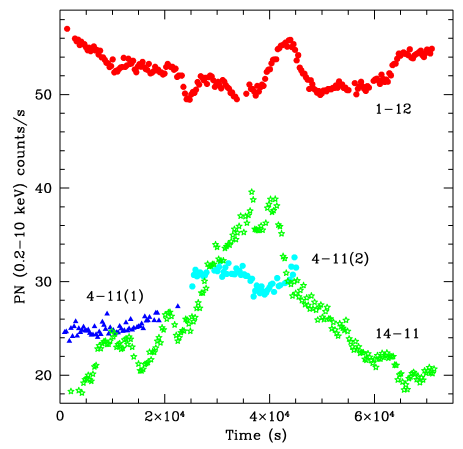
Figure 2: EPIC–PN [0.2–10] keV light curves of the four observational periods. The second exposure of November 4 is plotted as the continuation of the first. For plotting reasons, the December 1^st light curve, obtained in Timing mode, is rescaled down by a factor of 10 (see text). For clarity we do not plot the error bars (that in any case are comparable with the symbol sizes).

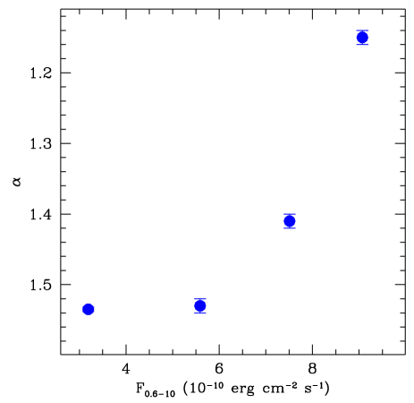
Figure 3: The best–fit power–law model spectral indexes versus the [0.6–10] keV flux. The source is harder when the [0.6–10] keV flux is higher.

In order to quantitatively estimate the source variability, we calculated the normalized excess variance of the 300 s binned light curves in different energy bands: [0.2–0.8] keV, [0.8–2.4] keV and [2.4–10] keV. We report our results in Table 3. According to Table 2 and Table 3, there is a trend indicating that the source is more variable while in a higher state of activity. We also found that the source is systematically more variable toward higher energies. This is not surprising in the framework of a standard leptonic model, (see e.g. Ghisellini et al. 1999), since the X–ray spectrum of an HBL should be produced via synchrotron emission. Harder X–rays are therefore produced by more energetic particles with smaller cooling timescales. Furthermore, since our hard X–ray spectra are systematically steeper than the soft X–ray spectra, a small change in the shape of the injected particle distribution will produce greater variations toward higher energies.

4.1 Hardness ratios

Obs. period	$\sigma^{2}_{rms}$
	($\times 10^{-3}$)
	[0.2–0.8] keV	[0.8–2.4] keV	[2.4–10] keV	[0.2–10] keV
4–11(1)	$0.33\pm 0.15$	$0.39\pm 0.30$	$2.53\pm 2.00$	$0.35\pm 0.15$
4–11(2)	$0.76\pm 0.19$	$1.23\pm 0.40$	$3.59\pm 1.91$	$0.78\pm 0.17$
14–11	$21.14\pm 2.24$	$40.96\pm 4.33$	$86.95\pm 10.04$	$32.76\pm 3.46$
1–12	$0.77\pm 0.08$	$1.73\pm 0.16$	$4.02\pm 0.43$	$1.07\pm 0.10$

Table 3: The excess variances of the 300 s binned light curves.

With these data obtained weeks apart, we have the possibility to check the spectral behaviour of the source both on long and on short timescales.

         

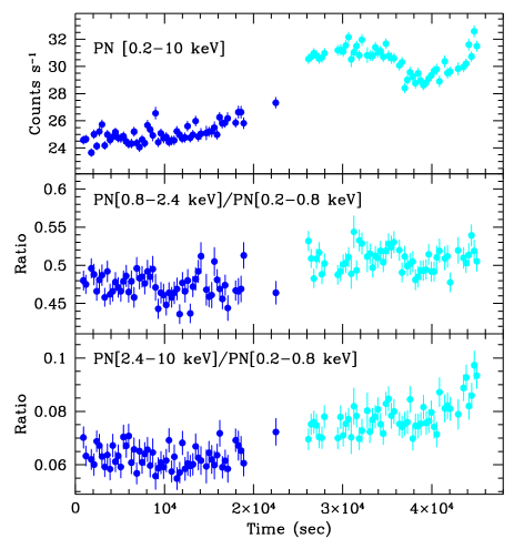
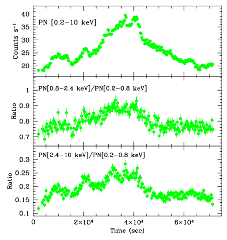
Figure 4: Left picture: November 4 EPIC–PN observation. Right picture November 14 EPIC–PN observation. The upper panel reports the PN [0.2–10] keV light curve, the mid panel the PN[0.8–2.4] keV/PN[0.2–0.8] keV hardness ratio and the lower panel the PN[2.4–10] keV/PN[0.2–0.8] keV hardness ratio. We plot together the two observations of November 4 (0136540301 and 0136540401).

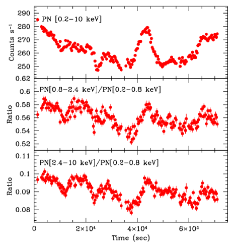
Figure 5: December 1^st EPIC–PN observation. The upper panels report the PN [0.2–10] keV 300 light curves, the mid panels the PN[0.8–2.4] keV/PN[0.2–0.8] keV hardness ratios and the low panels the PN[2.4–10] keV/PN[0.2–0.8] keV hardness ratios.

To study the long term trend, we compared the best–fit spectral indexes of the absorbed power–law model (which still provide reasonable fits to the data) to the total [0.6–10] keV fluxes reported in Table 2. We found that the X–ray spectra of Mkn 421 are harder when the fluxes are stronger (see Fig.3), as was already observed during other X–ray campaigns on Mkn 421 (see e.g. Fossati et al. 2000b; Sembay et al. 2002; Brinkmann et al. 2003) as well as on other similar sources (e.g. Mkn 501, Pian et al. 1998; 1ES 2344+514, Giommi et al. 2000; PKS 2155-304, Zhang et al. 2002a).
We checked this behaviour also on smaller timescales analysing the hardness ratios of light curves at different energies.
In Fig. 4 and Fig. 5 we plot the total [0.2–10] keV light curves (top panels), together with the [0.8–2.4] keV/[0.2–0.8] keV (mid panels) and the [2.4–10] keV/[0.2–0.8] keV hardness ratio (bottom panels) for each observing night.
In Fig. 4 and Fig. 5 it is clear that the hardness ratios are correlated with the [0.2–10] keV count rates: when the total flux increases the spectra become harder and conversely. This is verified both for long term variations (e.g. the slow flux increase observed during the whole November 4 observation, $\sim 4\times 10^{4}$ s), for short term variations (e.g. the small flare observed on December 1^st, $\sim 10^{4}$ s), for large events (e.g. the flare of November 14, flux variation $\gtrsim 100\%$) and for smaller events e.g. the same December flare ($\sim 10\%$).
This harder–when–stronger behaviour is also shown in the hardness ratio vs [0.2–10] keV count rate plots (see Fig. 6). The hardness ratios are correlated with the [0.2–10] keV flux: Mkn 421 becomes harder as the [0.2–10] keV flux increases. The null–correlation probability is always $<10^{-10}$.
To investigate the harder–when–stronger behaviour in more detail we concentrated on the November 14 and December 1^st observations, where two complete flares, different in amplitude and timescales, were detected.
Studying these two events, we investigated the spectral shape evolution during a whole flare, obtaining information on the particle acceleration/injection timescales (rising phase of the flare), on the cooling timescale (decaying section of the flare) and on the region geometry.
During the November 14 observation, the [0.2–10] keV counts increased by a factor larger than 2 and then decreased to the initial level in a total time of $\sim 7\times 10^{4}$ s. To avoid confusion caused by the small flares at the beginning and at the end of the observation, we excluded from the analysis the first $2.5\times 10^{4}$ s and the last 5000 s. For the observation of December 1^st, we analysed the small flare (lasting $1.4\times 10^{4}$ s) detected $\sim 4\times 10^{4}$ s after the beginning of the observation.
We rebinned these sections of the light curves in 2000 s and 1000 s bins, respectively. In Fig. 7, we plot the hardness ratios HR1 ([0.8–2.4] keV/[0.2–0.8] keV) and HR2 ([2.4–10] keV/[0.2–0.8] keV) as a function of the total [0.2–10] keV count rates. The rising phase data are plotted as filled circles and the decaying phase data as crosses.

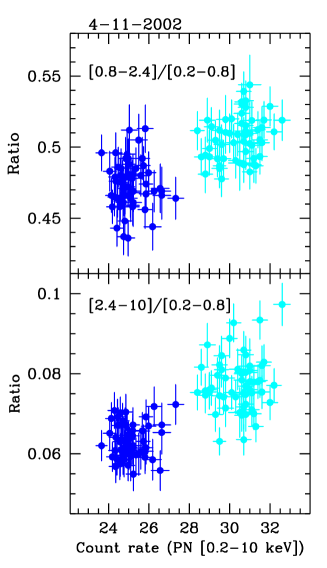
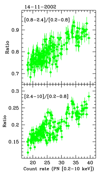
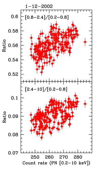
Figure 6: Upper panels: PN[0.8–2.4] keV / PN[0.2–0.8] keV ratios versus the [0.2–10] keV count rates. Lower panels: PN[2.4–10] keV / PN[0.2–0.8] keV ratios versus the [0.2–10] keV count rates. In the November 4 plot, we represent in dark grey the data of the first exposure and in light grey the data of the second exposure.

             

Figure 7: Hardness ratio/[0.2–10] keV count rate correlations for the flaring sections of the November 14 and December 1^st light curves (see text). HR1=[0.8–2.4 keV]/[0.2–0.8] keV; HR2=[2.4–10] keV/[0.2–0.8] keV. The rising phase data are plotted with circles, while the decaying phase data are plotted with crosses. Each temporal sequence starts from the data point marked with “1”.

Besides the above mentioned harder–when–stronger trend, in Fig. 7 we note a substantial different behaviour during the two flares: in the November 14 rising phase (circle symbols), the source is slightly harder than in the decaying phase (cross symbols), forming clockwise loop patterns. In the December 1^st flare, the source behaves in the opposite way: during the rising phase the source is systematically softer than in the decaying phase, forming a counterclockwise loop pattern.
In order to check the reality of these particular patterns, we performed a time resolved spectral analysis of the two flares.

4.2 Time resolved spectral analysis

We divided the November 14 observation in seven 10 ks sections and extracted the corresponding spectra. The extraction of the data and the filtering processes were performed as described in Section 2. We fitted each [0.6–10] keV spectrum with an absorbed power–law model keeping the absorption parameter fixed to the Galactic value. Because of the lower statistic, this model provides already a good representation of these spectra.
We performed the same analysis on the small flare of December 1^st. Since this observation was carried out in Timing mode, we have enough photon counts to split the short flare ($\sim 1.4\times 10^{4}$ s) in seven 2000 s sections and to extract well defined spectra from each of them. In Table 4 we report the best–fit spectral parameters for each temporal section of both flares.

Section	$\alpha$	ka	F0.6-10keVb	$\chi^{2}_{r}/d.o.f.$
			($\times 10^{-10}$)
14 November 2002, Obs. Id. 0136540701
1	$1.20\pm 0.01$	$0.199\pm 0.002$	7.44	1.28/125
2	$1.16^{+0.01}_{-0.02}$	$0.211\pm 0.001$	8.12	1.73/125
3	$1.10\pm 0.01$	$0.250\pm 0.002$	10.1	1.70/125
4	$1.03\pm 0.01$	$0.312\pm 0.002$	13.4	1.72/125
5	$1.17\pm 0.01$	$0.269^{+0.001}_{-0.002}$	10.3	1.35/125
6	$1.24\pm 0.01$	$0.222^{+0.001}_{-0.002}$	8.04	1.39/125
7	$1.23\pm 0.01$	$0.197\pm 0.002$	7.16	1.31/125
1 December 2002, Obs. Id. 0136541001
1	$1.597\pm 0.006$	$0.1027\pm 0.0004$	2.95	1.02/977
2	$1.574^{+0.006}_{-0.007}$	$0.1057^{+0.0003}_{-0.0004}$	3.08	0.96/998
3	$1.557\pm 0.006$	$0.1113^{+0.0003}_{-0.0004}$	3.27	1.15/1029
4	$1.517^{+0.007}_{-0.006}$	$0.115^{+0.0003}_{-0.0005}$	3.46	1.02/1026
5	$1.518\pm 0.006$	$0.1118^{+0.0003}_{-0.0004}$	3.36	1.09/1049
6	$1.535\pm 0.006$	$0.1066\pm 0.0004$	3.17	1.06/1038
7	$1.542^{+0.006}_{-0.007}$	$0.1029\pm 0.0004$	3.05	1.07/1033

Table 4: Best–fit parameters of the seven spectra extracted from the November 14, 2002 observation and from the flaring section of the December 1^st, 2002 observation, modelled with an absorbed power law. ^a: power law normalization (cts cm^-2 s^-1 keV^-1); ^b: erg cm^-2 s^-1.

The spectra become harder as the [0.6–10] keV flux increases and then soften to the initial shape as the source fades. This is shown also in Fig. 8 where we plot the best–fit spectral indexes versus the [0.6–10] keV flux.

             

Figure 8: We plot the best–fit spectral indexes $\alpha$ versus the [0.6–10] keV fluxes of the spectra extracted from seven sections of the November 14 exposure and from seven sections of the small flare occurred during the December 1^st observation. The spectra are modelled with an absorbed power law model. We plot the rising phase data with filled circles and the decaying phase data with crosses. The points marked with “1” are the first spectra of the temporal sequence.

Fig. 8 also shows the same clockwise (November 14) and counterclockwise loop patterns (December 1^st) obtained from the hardness ratio analysis.
These characteristic trends were already observed during previous campaigns on Mkn 421: performing a temporally resolved spectral analysis on ASCA data, Takahashi et al. (1996) were the first to observe a clockwise loop pattern which was interpreted as the signature of a soft lag ($\sim 1$h), i.e. hard X–ray variations leading soft X–ray variations. Fossati et al. (2000b), instead, were the first to find a counterclockwise loop pattern in a Mkn 421 flare observed by BeppoSAX, which they explained as the sign of a hard lag ($\sim 2-3$ h), i.e. soft X–ray variations leading hard X–ray variations. They confirmed this evidence performing also a discrete cross–correlation analysis. Using the same technique on different sections of an ASCA light curve of April 1998, Takahashi et al. (2000) found evidences of soft ($\sim 2000$ s), hard ($\sim 3400$ s) and of no lags.
Performing a discrete cross–correlation analysis on 4 XMM–Newton orbits, Sembay et al. (2002) did not found lags. They suggested that the previous detections were caused by systematic errors induced by gaps in the on–source time of low Earth orbit satellites such as BeppoSAX and ASCA. Brinkmann et al. (2003) re–analysed the same and other XMM–Newton data, dividing the light curves in sub–sections characterised by single flaring events. In different sections of the light curves, they found soft and hard lags as well as no lags, confirming the extremely complex behaviour of the source.
Similar behaviours were detected also in other sources, such as PKS 2155-304 (Kataoka et al. 2000; Zhang et al. 2002a) or BL Lacertae (Böttcher et al. 2003).

5 Delay determination

To check the presence and to estimate the amount of the temporal delays between flux variations in different energy bands, we performed two different kind of analysis. We concentrated on the two main variability features observed in the 4 EPIC–PN exposures, i.e. the large and structured flare seen on November 14, covering the whole XMM–Newton observation, and the small flare observed during the December 1^st observation.
The delay between two light curves is usually estimated by fitting the central peak of their cross–correlation function (CCF) with a Gaussian profile and taking the centroid position as the delay value. This technique, however, must be used cautiously: while it works properly for single, smooth and symmetrical flares, it can give unreal results when used on structured or asymmetrical light curves. In these cases, the CCF shape is deformed and the best–fit position of the Gaussian centroid will roughly be a weighted average of the delays between the several components or an index of the light curves asymmetry. Since our flares display complex shapes, in order to avoid confusion and wrong delay estimations, we fitted the CCF peaks with an asymmetrical model (e.g. Brinkmann et al. 2003), and checked the results by fitting the light curves with analytical models, to disentangle the various subcomponents. Comparing the locations of the maxima and the minima we obtained independent delay estimations. In the following Sections we will describe in detail these techniques and the results obtained.

5.1 Cross–correlation analysis

Since XMM–Newton provides good temporal coverage for the whole observing time, we performed the cross–correlations using the task CROSSCORR of the Xronos 5.19 package, based on a Fast Fourier algorithm which needs a continuous light curve, without interruptions. During the cross–correlation process, we filled the possible gaps with the running mean value calculated over the 6 closest bins. We check the results with the Discrete cross–correlation technique (DCC, Edelson & Krolik 1988) to verify the absence of distortions induced by the possible presence of such small gaps (note, however, that the DCC does not provide an error estimate on the peak position).
We performed the cross–correlations on the whole light curves of November 14 and of December 1^st as well as on their main flares. Therefore, for the November 14 exposure, we excluded the first $\sim 25$ ks and the last $\sim 10$ ks, while for the December 1^st we focused on the small feature, lasting $\sim 14$ ks, occurring after about half observation. Since the curves display several substructures, as a check we performed cross–correlations also on the excluded subsections.
We compared the [0.2–0.8] keV with the [0.8–2.4] keV and the [2.4–10] keV light curves, using different temporal binning (50, 100, 200 and 500 s). In order to estimate the position of the CCF peaks, i.e. the delay amounts, we fitted them with a constant + a skewed Gaussian model (the $\sigma$ below and above the Gaussian peak are different). This model, originally proposed and used by Brinkmann et al. (2003), accounts for the possible asymmetries of the CCF and therefore it accurately constrains their maximum. For the November 14 cross–correlations we fitted the central $\pm 15$ ks part of the CCF, to investigate its overall shape. We also fitted only the $\pm 5$ ks central part to obtain a more accurate peak position. For the December 1^st observation, we fitted only the central $\pm 5$ ks.
We remark, however, that the peak position is not always a correct delay estimator: for structured or asymmetrical light curves, it does not represent adequately the real temporal behaviour. In the first case, the possible delays in each variability event will be mixed together and the resulting delay will be an average value, obtained weighting each delay with its signal amplitude. In the second case, the CCF asymmetry can be a more relevant parameter, related to the slopes of the compared light curves (see below).
In Fig. 9 we plot the central peak of the cross–correlations performed on the main flares of the November 14 and of the December 1^st light curves. We also plot the Discrete cross–correlations (light grey data) and the best–fit constant + skewed Gaussian models (solid black lines). In Table 5 we report the best–fit peak positions and the weighted average of the $\sigma_{i}$ parameters for the cross–correlations and for the Discrete cross–correlations. Note, however, that the errors reported in Table 5 are underestimated since they account only for the statistic uncertainties on the skewed Gaussian parameters, which are also affected by two kinds of windowing effects. The first is related to the choice of the CCF section to be fitted, while the second is associated to the selection of the light curve intervals to be cross–correlated. Our simulations show that these effects can introduce uncertainties on the peak positions as large as 200–300 s, which are probably a more realistic error estimation than what reported in Table 5.

Curves id.	Lag (sec)				$<\sigma_{1}>$	$<\sigma_{2}>$
bin–time (s)	50	100	200	500	($10^{3}$ s)	($10^{3}$ s)
14 Nov 2002: whole curve. Central $\pm 15$ ks.
CCF I	$-890\pm 40$	$-750\pm 60$	$-830\pm 70$	$-760\pm 120$	$13.41\pm 0.15$	$12.76\pm 0.17$
DCC I	$-1030$	$-830$	$-740$	$-930$	$13.52$	$12.72$
CCF II	$-1860\pm 60$	$-1670\pm 80$	$-1730\pm 110$	$-1620\pm 160$	$15.04\pm 0.15$	$12.59\pm 0.20$
DCC II	$-2010$	$-1760$	$-1730$	$-1920$	$15.23$	$12.36$
14 Nov 2002: whole curve. Central $\pm 5$ ks.
CCF I	$-140\pm 90$	$-60\pm 110$	$-50\pm 180$	$-20\pm 250$	$4.00\pm 0.17$	$2.81\pm 0.20$
DCC I	$-90$	$-80$	$-20$	$-50$	$4.04$	$2.66$
CCF II	$-180\pm 130$	$-180\pm 180$	$-120\pm 260$	$-90\pm 360$	$7.20\pm 0.40$	$3.02\pm 0.27$
DCC II	$-80$	$-170$	$-60$	$-60$	$7.40$	$2.79$
14 Nov 2002: main flare. Central $\pm 15$ ks.
CCF I	$-600\pm 40$	$-560\pm 60$	$-630\pm 90$	$-640\pm 140$	$9.04\pm 0.06$	$7.84\pm 0.07$
DCC I	$-770$	$-700$	$-620$	$-790$	$9.10$	$8.01$
CCF II	$-1390\pm 60$	$-1350\pm 90$	$-1340\pm 130$	$-1410\pm 190$	$10.46\pm 0.07$	$8.24\pm 0.09$
DCC II	$-1580$	$-1550$	$-1460$	$-1370$	$10.39$	$8.38$
14 Nov 2002: main flare. Central $\pm 5$ ks
CCF I	$-210\pm 90$	$-140\pm 140$	$-110\pm 190$	$-80\pm 300$	$3.97\pm 0.18$	$2.95\pm 0.21$
DCC I	$-220$	$-160$	$-90$	$-150$	$4.30$	$3.14$
CCF II	$-410\pm 170$	$-290\pm 260$	$-250\pm 340$	$-220\pm 500$	$8.31\pm 0.56$	$4.01\pm 0.43$
DCC II	$-340$	$-380$	$-240$	$-350$	$8.58$	$4.30$
1 Dec 2002: whole curve
CCF I	$160\pm 50$	$220\pm 60$	$250\pm 90$	$230\pm 120$	$2.41\pm 0.07$	$4.04\pm 0.06$
DCC I	$90$	$160$	$200$	$120$	$2.49$	$4.03$
CCF II	$530\pm 80$	$570\pm 100$	$610\pm 130$	$740\pm 220$	$2.87\pm 0.13$	$6.04\pm 0.18$
DCC II	$560$	$570$	$590$	$400$	$2.77$	$6.08$
1 Dec 2002: flare
CCF I	$430\pm 50$	$470\pm 60$	$490\pm 80$	$480\pm 110$	$3.29\pm 0.10$	$3.85\pm 0.08$
DCC I	$400$	$460$	$480$	$450$	$3.24$	$3.83$
CCF II	$950\pm 80$	$950\pm 100$	$940\pm 130$	$860\pm 180$	$3.39\pm 0.15$	$4.34\pm 0.10$
DCC II	$1040$	$960$	$920$	$840$	$3.32$	$4.29$

Table 5: Best–fit parameters of the constant + skewed Gaussian model reproducing the cross–correlation (CCF) peaks. We cross–correlated the whole light curves of November 14, of December 1^st and their main flares. We compared the [0.2–0.8] keV light curves to the [0.8–2.4] keV (Id. I) and to the [2.4–10] keV light curves (Id. II). We also performed a Discrete cross–correlation (DCC) on the same curves. We reproduced the central $\pm 15$ ks and $\pm 5$ ks of the November 14 CCF and the central $\pm 5$ ks of those of December 1^st. Negative lags mean that the variations in the hard X–ray band lead those in the soft X–ray band. The reported skewed Gaussian $\sigma_{i}$ are the weighted averages of the four amplitudes.

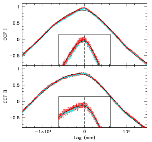
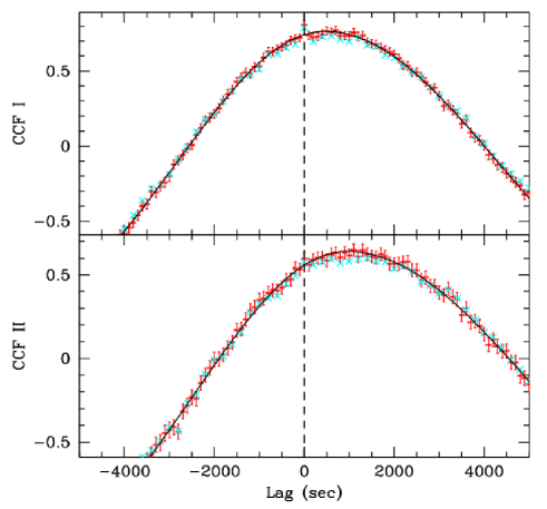
Figure 9: The left panel shows the central $\pm 15$ ks of the cross–correlations performed on the flare of November 14. The insert shows only the central $\pm 5$ ks, with a better fit of the peaks. The central $\pm 5$ ks of the cross–correlations performed on the flare of December 1^st is shown in the right panel. The light curves were rebinned in 100 s bins. CCF I: PN [0.8–2.4 keV] vs PN [0.2–0.8 keV]. CCF II: PN [2.4–10 keV] vs PN [0.2–0.8 keV]. We show in dark grey the cross–correlation data and in light grey the Discrete cross correlation data. The solid black line is the best–fit skewed Gaussian model (the insert data are fitted independently).

We summarize the results of the cross–correlation analysis as follows:

• the results obtained from differently binned light curves are consistent with each other. Furthermore, the Discrete cross–correlation results are fully consistent with those of the cross–correlations. The best–fit parameters relative to the two techniques, in fact, are very similar

• the lags obtained cross–correlating the whole curves are similar (November 14) or smaller (December 1^st) than those obtained considering only the flares: the delays are probably produced during the main flux variations. This is confirmed by the absence of significant lags in the other sections of the light curves, as evidenced, e.g. by the lack of clear loop patterns in the hardness ratio versus count rate plots corresponding to the minor flares of November 14 (peaking at $\sim 10000$ s, $\sim 20000$ s and at $\sim 62000$ s), by the cross–correlations performed on these intervals and by reproducing the curves with analytical models (see next Section)

• November 14: the peak positions obtained for the $\pm 15$ ks central part of the CCF are not consistent with zero delays. However, this is due to the strong asymmetry of the CCFs that are not well fitted even by a skewed Gaussian model. On this time interval the fit is dominated by the wings of the CCF and the peak is not well fitted. A more accurate position of the peaks are obtained by fitting only the central $\pm 5$ ks of the CCFs. In this case the position of the peaks are consistent with $\sim$ zero delay (see the inserts in the left panel of Fig. 9). However, they are asymmetrical, being broader toward negative lags. Thus, we have to explain a CCF that has a zero lag delay, but an asymmetrical shape. A possibility could be that this peculiar shape of the CCF is due to variability patterns present in both light curves, peaking simultaneously but with different rising and/or decaying time scales. For instance, in the case of blazars we can imagine to have a flare characterised by a linear increase, i.e. dominated by geometric effects, followed by an exponential decay with different $\tau$ at different frequencies (i.e. dominated by cooling effects). To test this possibility, we generated simulated flare light curves, assuming different rising and decay time scales, but a simultaneous peak position for the flare in the two light curves. From their cross-correlation we obtained CCF that are very similar to the ones shown in Fig. 9. We also added a Gaussian feature to reproduce the small flare that is present in the real light curves at $\sim 19000$ s (see peak 3.2, next Section): this extra feature, however, has the same properties in all bands and does not introduce significant effects. Having shown that with such an analytical model (linear rising + exponential decay + a Gaussian feature) we can reproduce the observed CCF, we fitted it to our light curves. With the best–fit parameters, we generated 500 s binned light curves, attributing to each point the uncertainty of the corresponding real one (see Fig. 10, left panels). Then we cross–correlated these model–generated light curves and fitted the CCF peaks with a skewed Gaussian model as we did with the real light curves (see Fig. 10, right panels). The best–fit parameters are consistent with those reported in Table 5. Similar results are obtained also using shorter temporal bins, so here we show only the case of the 500 s bins. Thus, with this simple analytical model we can reproduce both the observed flare light curves and the resulting CCF.
  Clearly, for this event the harder X–ray light curves have a steeper increase (i.e. a hardening of the spectrum) and a faster decay (i.e. a softening of the spectrum), leading on average those at softer energies. Therefore, even if the peaks are simultaneous, the different slopes of the flares will produce a sort of soft lag. As a first indication of this lag, we will consider the difference between the halving times of the fitted exponential curves. In Table 6 we summarize our results.

• December 1^st: the cross–correlations are more symmetrical and their maxima are located at positive lags (see the right picture of Fig. 9). Since this flare is quite smooth, the cross–correlation shapes are probably originated by light curves peaking at different times. In this case, the peak positions of the best–fit skewed Gaussian give a straightforward estimate of the delays. During this flare, therefore, the [0.2–0.8] keV variations lead those at [0.8–2.4] keV and at [2.4–10] keV by $450\pm 30$ s and by $950\pm 60$ s, respectively (these values are the weighted mean of those reported in Table 5). This behaviour can be produced, for instance, by an energy dependent particle acceleration: lower energy particle are produced sooner (see the Discussion).

• we confirm the results of the hardness ratio and time resolved spectral analysis: there are delays between flux variations at different energies. During the November 14 observation, when the spectral evolution was characterised by a clockwise loop pattern, the harder X–ray fluxes were decaying faster. During the small flare of December 1^st, instead, when we observed counterclockwise loop patterns, the mid and the hard X–ray flare peaks were delayed by $450\pm 30$ s and by $950\pm 60$ s, respectively.

• comparing light curves of different energy range, the delays are larger for a larger difference between the energy ranges considered: the temporal lags between the [0.2–0.8] keV and the [2.4–10] keV light curves are larger than those between the [0.2–0.8] keV and the [0.8–2.4] keV curves.

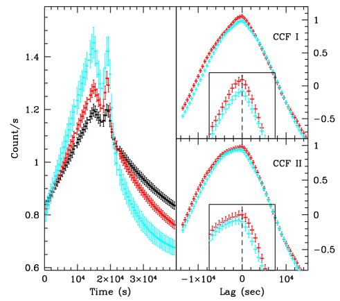
Figure 10: Left panel: 500 s binned light curves generated from the best–fit models to the main flare of November 14 (see text). We show the [0.2–0.8] keV data in black, the [0.8–2.4] kev data in dark grey and the [2.4–10] keV data in light grey. The model is characterised by a linear increase and by an exponential decay, to which we add a Gaussian profile reproducing the small flare at $\sim 19000$ s. The peak position is fixed at 15000 s. Right panels: we show the cross–correlations obtained from the real 500 s binned light curves (dark grey) and from the curves in the left panel (light grey). CCF I: PN [0.8–2.4 keV] vs PN [0.2–0.8 keV]. CCF II: PN [2.4–10 keV] vs PN [0.2–0.8 keV]. In the inserts we show the peak regions.

Energy band	e-folding time	Halving time	Lag
(keV)	($10^{4}$ s)	($10^{4}$ s)	($10^{4}$ s)
$[0.2-0.8]$	$25.2\pm 0.9$	$17.5\pm 0.6$
$[0.8-2.4]$	$16.9\pm 0.8$	$11.7\pm 0.6$	$-5.8\pm 0.8$
$[2.4-10]$	$8.3\pm 1.1$	$5.8\pm 0.8$	$-11.6\pm 1.0$

Table 6: Best-fit e-folding time of the exponential model reproducing the flare decay of November 14 in the three energy bands. We also report the respective halving times and their differences between the soft and the two harder energy bands.

In the next Section we will check these results by fitting the light curves with analytical models.

5.2 Modelling the light curves

We rebinned the November 14 light curve and the December 1^st flare using 500 s and 200 s bins, respectively. Since the November 14 curve was very structured, we fitted it with the linear increase+exponential decay model described in the previous Section + 4 Gaussian profiles (see Fig. 11). The asymmetrical curve and one Gaussian were aimed at reproducing the large central flare (henceforth peak 3): the first (peak 3.1 in Fig. 11) representing the main, average variation and the second one describing the clear bump at $\sim 41000$ s (peak 3.2). The other Gaussian were used to model the small features at $\sim 10000$ s (peak 1), $\sim 20000$ s (peak 2) and $\sim 62000$ s (peak 4) from the beginning of the observation. We were able to reproduce the light curves leaving all the parameters free to vary in the best fit procedure.

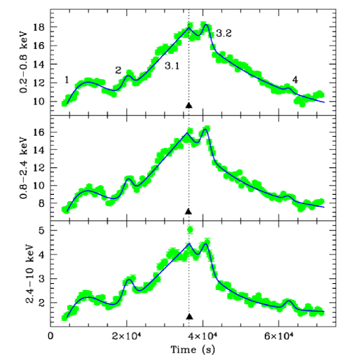
Figure 11: November 14, 2002: PN [0.2–0.8] keV, [0.8–2.4] keV and [2.4–10] keV 500 s rebinned light curves of Mkn 421 (the y–axis unit is count/s). We plot the best–fit model as a solid black line: we used a linear increase+exponential decay curve summed to 4 Gaussian profiles. The black filled triangles represent the peak position of flare 3.1 in the three bands: they are nearly simultaneous.

The December 1^st flare, instead, was quite smooth and we fitted it with a 4^th degree polynomial peaking at $\sim 11000$ s from the beginning of the temporal window (see Fig.12). We chose this profile because it well reproduce the light curve asymmetries. However, to estimate the uncertainties on the peak positions, we fitted the flare also with a constant plus a Gaussian model. The results obtained with the two models are very similar. In Table 7 we report all the best–fit parameters.

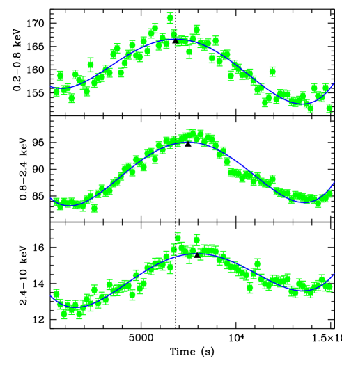
Figure 12: December 1^st, 2002: PN [0.2–0.8] keV, [0.8–2.4] keV and [2.4–10] keV 200 s rebinned light curves of Mkn 421. We plot the small flare detected at about half observation. The solid line represents the best–fit 4^th degree polynomial model. The dotted vertical line represents the [0.2–0.8] keV peak position and the black filled triangles indicate the peak position of the three curves. It is clear that the high energy curve peaks are delayed.

14 November
Feature	Time			Lag
	[0.2–0.8] keV	[0.8–2.4] keV	[2.4–10] keV	$t_{2}-t_{1}$	$t_{3}-t_{1}$
	(s)	(s)	(s)	(s)	(s)
Peak 1	$6990^{+300}_{-330}$	$6810^{+240}_{-270}$	$6980^{+340}_{-400}$	$-180^{+380}_{-430}$	$-10^{+450}_{-520}$
Peak 2	$20220^{+250}_{-260}$	$20330^{+160}_{-170}$	$20470^{+160}_{-180}$	$+110^{+300}_{-310}$	$+250^{+300}_{-320}$
Peak 3.1	$36360^{+330}_{-430}$	$36220^{+240}_{-640}$	$36550^{+220}_{-410}$	$-140^{+410}_{-770}$	$+190^{+400}_{-590}$
$\sigma_{1}$	$25170^{+980}_{-910}$	$16260^{+880}_{-810}$	$9560^{+800}_{-680}$
Peak 3.2	$41040\pm 220$	$40860\pm 130$	$41000\pm 200$	$-140\pm 260$	$-40\pm 300$
Peak 4	$62680^{+670}_{-560}$	$62860^{+530}_{-480}$	$62670\pm 290$	$+180^{+850}_{-740}$	$-10^{+730}_{-630}$
1 December
Flare start	$790$	$1210$	$1550$	$+420$	$+760$
Flare peak	$6810$	$7470$	$7950$	$+660$	$+1140$
Peak (Gauss.)	$6760\pm 100$	$7430\pm 80$	$8010\pm 160$	$+670\pm 130$	$+1250\pm 180$
Flare end	$13490$	$13610$	$13510$	$+120$	$+10$

Table 7: Maxima and minima of the best–fit models of the November 14 and of the December 1^st flares in three different energy bands. The November 14 and the December 1^st light curves are binned in 500 s and 200 s intervals, respectively. For the November 14 observation we report also the best-fit e-folding time of the exponential decay model. For the December observation we give the start and stop time of the flare and the flare peak (using two different models, see text). In columns 5 and 6 we report the delays between the features of the medium [0.8–2.4] keV (Col. 5) and the hard [2.4–10] keV (Col. 6) light curves with respect to those of the soft [0.2–0.8] keV light curve.

During the November 14 observation the source behaved in a complex way:

• both peak 1 (at $\sim 10000\,$s) and peak 2 (at $\sim 20000\,$s) occur almost simultaneously in the three bands; all delays are consistent with zero.

• even the two subcomponents forming the third, large flare do not show significant peak shifts. We remark, however, the large differences in the decay slopes of the peak 3.1. Although the flare peaks are almost simultaneous, the flux increase is larger in the harder X–ray bands and the following decay is much faster. As shown in the previous section, this produces the distortions observed in the cross–correlations.

• again the small peak 4 occurs almost simultaneously in the three bands, although with larger uncertainties due to the fact that this event is well pronounced in the harder energy band but not in the other two.

The absence of delays at the peaks 1, 2 & 4 is confirmed by the lack of loop patterns in the corresponding hardness ratio vs count rate plots. We conclude therefore that the clockwise loop patterns evidenced in Section 4.1 and Section 4.2 are connected with the presence of soft lags, mainly caused by the different slopes of the peak 3.1. The smaller substructures are not characterised by the presence of significant delays. As expected (see previous section), we find that the slope difference between the [0.2–0.8] keV and the [2.4–10] keV light curves is larger than that between the [0.2–0.8] keV and the [0.8–2.4] keV light curves.
The situation is different for the isolated flare of December 1^st: the [0.2–0.8] keV leads the mid and the hard curves both at the beginning ($\sim 420$ s and $\sim 760$ s, respectively) and at the peak of the flare ($\sim 660$ s and $\sim 1140$ s), as confirmed also by the constant + Gaussian model. The delay of the [2.4–10] keV variation is significantly larger than that of the [0.8–2.4] keV curve and they are consistent with those obtained through the cross–correlations. The fade of the flare, instead, seems to stop almost simultaneously in the three bands.
The light curves are very structured and our models do not exactly follow the small substructures that are present. However, the use of more complex models is beyond our goal, that is to determine the existence and the amount of delays between the main variability features in different energy bands. The lags reported in Table 7 are therefore average values mixing the contributions of the light curve substructures, in line with the results obtained from the cross-correlation analysis.

6 Discussion

We observed X–ray spectral evolution during two complete flares of Mkn 421 through a hardness ratio and a time resolved spectral analysis. This was clearly shown by the presence of hysteretic patterns in the hardness ratio vs count rate plots and in the spectral index vs flux plots. Such characteristic patterns are usually explained as the signatures of temporal delays between different energy light curves (see e.g. Takahashi et al. 1996). Then, we used two techniques to check the reality and to estimate the amount of such possible lags; a) we performed a cross–correlation analysis and b) we reproduced the light curves with analytical models to compare the positions of the maxima. We confirmed the presence of the temporal lags. More precisely, we found soft lags in the observation of November 14, produced by different variability rates during a single, even if structured flare (peak 3.1 in Fig. 11), which cannot be further split. In the observation of December 1^st we observed the opposite behaviour: a small, smooth flare is characterised by large hard lags. We found also that the delays between the [0.2–0.8] keV and the [2.4–10] keV bands are larger than those between the [0.2–0.8] keV and the [0.8–2.4] keV bands. They must be produced by energy dependent mechanisms like, for instance, the particle cooling and acceleration.
Following the treatment of Zhang et al. (2002a), we can express the cooling timescale $t_{cool}$ and the acceleration timescale $t_{acc}$ in the observer frame as a function of the photon energy $E$ (in keV) as:

$$t_{cool}(E)=3.04\times 10^{3}(1+z)^{1/2}B^{-3/2}\delta^{-1/2}E^{-1/2}s$$ (2)

$$t_{acc}(E)=9.65\times 10^{-2}(1+z)^{3/2}\xi B^{-3/2}\delta^{-3/2}E^{1/2}s$$ (3)

where $z$ is the redshift of the source, $B$ is the magnetic field in Gauss, $\delta$ is the Doppler factor of the emitting region and $\xi$ is a parameter indicating the acceleration rate of electrons (see Zhang et al., 2002a). As evidenced by equations 2 and 3, the cooling and the acceleration mechanisms behave oppositely with respect to the photon energy $E$: higher energy particles cool faster and accelerate slower. Another important timescale which could be involved in the production of the delays is the light crossing time of the emitting region $t_{esc}$. In fact, Ghisellini, Celotti & Costamante (2002) suggested that the synchrotron peak of HBL objects (and therefore of Mkn 421) is produced by particles with cooling time $t_{cool}=t_{inj}\sim t_{esc}$, where $t_{inj}$ is the particle injection/acceleration timescale. In an internal shock scenario $t_{inj}$ is very similar to $t_{esc}$.
A different balancing of these characteristic timescales, $t_{cool}$, $t_{acc}$ and $t_{esc}$ can account for the observed temporal lags.

• November 14: the November 14 light curve is very structured, showing several small features. However, only the large flare 3 is characterised by clear lags, mainly caused by the different slopes of the peak 3.1. Since the source is displaying a soft spectrum above 0.6 keV, with spectral index $\alpha\sim 1.13$, we are very close to the synchrotron peak, which could be even located inside our softer energy band ([0.2–0.8] keV). This implies that $t_{cool}\sim t_{esc}>>t_{acc}$ (since $t_{acc}=t_{cool}$ at the highest observed synchrotron energy $E_{max}$).
  In this case, we assume a particle acceleration, that produces a spectral hardening and leads to simultaneous peaks, followed by a decay dominated by cooling effects. Since the highest energy particles suffer the quickest cooling, we will observe soft lags and clockwise loop patterns in the spectral index vs flux plots. The soft lags and their frequency dependence observed during this flare can be attributed to the frequency dependence of $t_{cool}$.

• December 1^st: the small flare after about half observation shows large hard lags. In this case the source spectrum is softer ($\alpha\sim 1.5$) than in November 14. We are therefore closer to $E_{max}$, where $t_{cool}\sim t_{acc}$. In this case we can assume $t_{esc}>>t_{cool}\sim t_{acc}$: the information about the occurrence of a flare propagates from lower to higher energies, as particles are gradually accelerated, while the decay of the flare could be dominated by the particle escape effects, which can be assumed achromatic. Then we will observe hard lags and counterclockwise loop patterns, produced by real delays at the peak of the flares. In this case, the observed hard lag will be generated by the frequency dependence of $t_{acc}$.
  This scenario is supported by the shape of the loop patterns shown in Fig. 7 (right panels): as the flux begins to increase, the spectrum softens. This can be explained as an effect of the progressive acceleration: the spectrum initially steepens because electrons cannot be accelerated to higher energies, yet.

The presence of soft and hard lags can therefore be explained in the framework of different cooling or acceleration timescales. A similar conclusion was reached also by other authors, by solving the particle and photons continuity equations (see e.g. Kirk, Rieger & Mastichiadis 1998).
The detection of lags can shed some light on the acceleration as well as on the cooling mechanisms and provide a powerful tool to constrain the physical parameters of the source. In fact, if the soft lags $\tau_{soft}$ of November 14 are produced by cooling effects, ($\tau_{soft}=t_{cool}(E_{s})-t_{cool}(E_{h})$) and the hard lags of December 1^st are produced by acceleration effects ($\tau_{hard}=t_{acc}(E_{h})-t_{acc}(E_{s})$), we can estimate the physical properties of the emitting region through the equations

$$B\leavevmode\nobreak\ \delta^{1/3}=209.91\Big{(}\frac{1+z}{E_{s}}\Big{)}^{1/3}\Big{[}\frac{1-(E_{s}/E_{h})^{1/2}}{\tau_{soft}}\Big{]}^{2/3}G$$ (4)

$$B\leavevmode\nobreak\ \delta\leavevmode\nobreak\ \xi^{-2/3}=0.21(1+z)E^{1/3}_{h}\Big{[}\frac{1-(E_{s}/E_{h})^{1/2}}{\tau_{hard}}\Big{]}^{2/3}G$$ (5)

where $E_{s}$ and $E_{h}$ are the mean energies in the corresponding energy bands, taking into account the power–law shape of the spectrum (Zhang et al., 2002a).
Since the amount of the lags changes when comparing different couples of light curves, we have the opportunity to check the reality of this scenario. If our assumptions are correct, assuming that a flare is produced by a single electron population, using the lags between different couples of light curves in the equations 4 and 5, we should obtain the same emitting region characteristics. For the flare of November 14, we used the delays obtained from the halving times differences of the simulated light curves, while for that of December 1^st we used the difference between the cross–correlation peak positions. In Table 8 we report the assumed parameters and the results. For the December 1^st lags, we do not consider the uncertainties shown in Table 5 since they are probably underestimated: we will assume more conservative error values of 200 s.

$E_{1}$	$E_{2}$	$E_{3}$	$\tau_{12}$	$\tau_{13}$	$B_{12}$	$B_{13}$
(keV)	(keV)	(keV)	(s)	(s)	(G)	(G)
November 14 soft lag
0.42	1.44	5.19	5800	11600	$0.24\pm 0.02\leavevmode\nobreak\ \delta_{10}^{-1/3}$	$0.21\pm 0.01\leavevmode\nobreak\ \delta_{10}^{-1/3}$
December 1 hard lag
0.40	1.38	4.87	$450\pm 200^{*}$	$950\pm 200^{*}$	$0.53\pm 0.12\leavevmode\nobreak\ \delta_{10}^{-1}\xi_{5}^{2/3}$	$0.65\pm 0.08\leavevmode\nobreak\ \delta_{10}^{-1}\xi_{5}^{2/3}$

Table 8: To evaluate the mean energies of the three analysed bands, we used the spectral indexes of the best–fit power–law models in the [0.6–10] keV ranges ($\alpha=1.15\pm 0.01$ and $\alpha=1.535\pm 0.003$). We do not report the errors on the mean energies which are of the order of $10^{-4}$ keV. The notations $\delta_{10}$ and $\xi_{5}$ mean ($\delta/10$) and $\xi/10^{5}$, respectively. ^∗: since the uncertainties reported in Table 5 are probably underestimated, we assumed more conservative errors of 200 s.

The data reported in Table 8 are consistent with the proposed scenario: the observed soft lags are likely to be produced by the particle cooling and the hard lags by a progressive acceleration. The difference between the magnetic fields obtained from the November 14 and for the December 1^st data, probably reflects our poor knowledge on the details of the real particle acceleration mechanism working in blazars.
It is interesting to point out that the magnetic field values reported in Table 8 ($B\sim 0.2-0.65$ G) are higher than those obtained modelling the multiwavelength SEDs of the source with SSC models. These models, in fact, require weak magnetic fields to reproduce the observed TeV emission (e.g. Ghisellini, Celotti & Costamante 2002). This inconsistency could be caused by the techniques employed to estimate the lags, which provide only lower limits of the “real” delays when applied to light curves displaying substructures with different behaviours, or by the poor knowledge of the acceleration parameter $\xi$ (which we arbitrarily assumed to be $10^{5}$ in the case of the smooth flare of December 1^st).

7 Conclusion

We presented the spectral and temporal analysis of 3 XMM–Newton observations of Mkn 421. We resume here the main results:

1. The X–ray spectra of Mkn 421 are soft and steepen toward higher energies: the November 4 spectra are best fitted by a softening parabolic model, while the November 14 and the December 1^st data are best fitted by convex broken power–laws. We are probably observing synchrotron emission from a range above the low energy peak of the SED, which, however, should be located very close to our lower limit (e.g. in November 14, $\alpha_{1}=1.13$).

2. The hardness ratio analysis of two complete, different flares occurring in November 14 and in December 1^st shows the presence of strong spectral evolution. Besides presenting a clear harder–when–stronger correlation, the hardness ratio vs count rate plots display characteristic loop patterns, which are the signature of temporal delays between flux variations in different energy bands. During the November 14 flare, the loop pattern rotates clockwise, suggesting the presence of soft lags (see e.g. Takahashi et al. 1996), while during the December 1^st flare, the loop pattern rotates counterclockwise (hard lags, see e.g. Fossati et al. 2000b). These results were also confirmed by Brinkmann et al. (2003) using high quality XMM–Newton data.

3. We confirmed the results of the hardness ratio analysis performing a time resolved spectral analysis. We observed again the loop patterns rotating clockwise and counterclockwise in November 14 and in the flare of December 1^st, respectively.

4. We verified the presence of the delays performing a cross–correlation analysis. We found that the lags are mainly produced by the complete flares of November 14 and December 1^st, while the rest of the light curves do not show delays. In the first case, the flare peaks are simultaneous but are characterised by different slopes, producing, on the average, soft lags. In the second case, the flare peaks display significant hard lags. The clockwise loop patterns are then associated with the presence of soft lags, while the counterclockwise loop patterns are associated with hard lags. We also found that the delays increase with the energy difference between the compared light curves.

5. We fitted the November 14 and the December 1^st flares at different energies with analytical light curve models, to split them in their subcomponents. We estimated the delays for each component obtaining agreement with the results of the cross–correlation and of the hardness ratio analysis. The main flare of November 14 does not display peak delays, but it is characterised by different slopes, producing, on the average, soft lags. The other components of this light curve do not show significant delays. The December 1^st flare is characterised by hard lags.
   The complex behaviours of the subcomponents can be explained as produced by different emitting regions. This is naturally accounted by the internal shock model proposed by Ghisellini (1999) and by Spada et al. (2001).

6. We presented a scenario to explain the presence of soft or hard lags as a consequence of different cooling and acceleration timescales. The results of the data analysis are quite consistent with this picture, suggesting that the frequency dependence of the synchrotron cooling is probably responsible for the November 14 soft lags. Also the hard lags in the December 1^st flare are roughly compatible with the assumed acceleration mechanism.

We demonstrated that the hardness ratio and the temporally resolved spectral analysis are very powerful tools to establish the presence of temporal lags between light curves at different energies. With the cross–correlation technique we were able to estimate the amount of the delays. It is however important to point out that this technique must be used cautiously. While it is very reliable when applied to single smooth and symmetrical flares, it can produce mixed results when applied to the complex and structured light curves of blazars as a whole. A careful check of the behaviour of the single components must be performed before using the cross–correlation results to test the blazar models.