Dealing with systematics in cosmic shear studies: new results from the VIRMOS-Descart Survey

We present a reanalysis of the VIRMOS-Descart weak lensing data, with a particular focus on different corrections for the variation of the point spread function anisotropy (PSF) across the CCDs. We show that the small scale systematics can be minimised, and eventually suppressed, using the $B$ mode (curled shear component) measured in the corrected stars and galaxies. Updated cosmological constraints are obtained, free of systematics caused by PSF anisotropy. To facilitate general use of our results, we provide the two-points statistics data points with their covariance matrices up to a scale of one degree. For the normalisation of the mass power spectrum we obtain $\sigma_{8}=(0.83\pm 0.07)\left(\Omega_{M}/0.3\right)^{-0.49}$. The shape parameter $\Gamma$ was marginalised over $\Gamma\in[0.1,0.3]$ and the mean source redshift $z_{s}$ over $[0.8,1.0]$. The latter is consistent with recent photometric redshifts obtained for the VIRMOS data and the preliminary spectroscopic redshifts from the VIRMOS-VVDS survey. The quoted $68\%$ contour level includes all identified sources of error. We discuss the possible sources of residual contamination in this result: the effect of the non-linear mass power spectrum and remaining issues concerning the PSF correction. Our result is compared with the first release of the Wilkinson Microwave Anisotropy Probe data. It is found that Cold Dark Matter models with a power law primordial power spectrum and high matter density $\Omega_{M}>0.5$ are excluded at 3-$\sigma$.

1 Introduction

Weak gravitational lensing by large scale structure (i.e., cosmic shear) directly probes the matter distribution and complements studies of the local universe based on the light (galaxy) distribution alone. Its sensitivity to the dark matter power spectrum and the geometry of the universe are key ingredients for breaking cosmological parameters degeneracies associated with other experiments such as Cosmic Microwave Background (Spergel et al. 2003) and the Type Ia supernovae (Riess et al. 1998; Perlmutter et al. 1999). This powerful application has motivated a first generation of surveys and the field has made significant strides forward in the past four years. A compilation of the first measurements (Bacon et al. 2000; Kaiser et al. 2000; Van Waerbeke et al. 2000; Wittman et al. 2000) and of the more numerous recent ones, with discussions of the strength and weaknesses of weak lensing, have been recently reviewed by a number of papers (e.g., Van Waerbeke & Mellier 2003; Réfrégier 2003; Hoekstra 2003a).

Cosmic shear studies are now entering the second phase as new surveys, such as the Canada-France-Hawaii Telescope Legacy Survey (CFHTLS) aim to cover areas of sky that are an order of magnitude larger than current data sets. These second generation surveys can provide constraints on a range of cosmological parameters, with a precision that is comparable to current CMB experiments. However, the success hinges on the ability to control and correct for observational systematics. Indeed, there are several technical issues remaining, concerning the point spread function (PSF) correction, the galaxy shape analysis and the prediction of the non-linear power spectrum. Whether this is possible is still debated.

One of the best ways to proceed is to learn from experience obtained from the first generation surveys. The VIRMOS-Descart survey that will be discussed below provides an excellent means to do so. It has already produced several results of cosmological interest (Van Waerbeke et al. 2002; Hoekstra et al. 2002; Bernardeau, Mellier & van Waerbeke 2002; Pen, van Waerbeke & Mellier 2002; Pen et al. 2003b), but showed a non-zero B-mode signal at all scales, which has limited its use for precise cosmological applications. This systematic residual signal is indeed an important noise contribution. It is therefore timely to understand the cause of B-mode generation in cosmic shear data and to provide better and more reliable tools to handle them.

The purpose of this paper is to put the various issues mentioned above into perspective, and discuss their relevance to future surveys. We do so by presenting a reanalysis of the VIRMOS-Descart data, taking advantage of the latest improvements in PSF correction and a better estimate of the redshift distribution of sources based on recent spectroscopic data in the VIRMOS-Descart fields obtained by the VIRMOS-VLT Deep Survey (VVDS). Tables providing results of the best-corrected shear signals as function of angular scale as well as errors are also given in this paper to help further joint analyses using complementary cosmological data sets.

This paper is organised as follows: Section 2 defines the notation and introduces the statistical quantities to be used. Section 3 provides a summary of the VIRMOS survey. In Section 4 we discuss the impact of PSF correction on the cosmic shear signal. Sections 5 and 6 show the new results from the VIRMOS-Descart survey.

2 Theory

For self-consistency and in order to define the notations, we briefly outline the revelant quantities used in this paper. More detailed calculations and explanations can be found in recent reviews. Following the notation in Schneider et al. (1998), we define the power spectrum of the convergence $\kappa$ as

$$P_{\kappa}(k) = {9\over 4}\Omega_{0}^{2}\int_{0}^{w_{H}}{{\rm d}w\over a^{2}(w)}P_{3D}\left({k\over f_{K}(w)};w\right)\times$$ (1)

$$\left[\int_{w}^{w_{H}}{\rm d}w^{\prime}n(w^{\prime}){f_{K}(w^{\prime}-w)\over f_{K}(w^{\prime})}\right]^{2},$$

where $f_{K}(w)$ is the comoving angular diameter distance out to a distance $w$ ($w_{H}$ is the horizon distance), and $n(w(z))$ is the redshift distribution of the sources given in Eq.(12). $P_{3D}(k)$ is the 3-dimensional mass power spectrum (computed from a non-linear estimation of the dark matter clustering, see e.g. Peacock & Dodds (1996); Smith et al. (2003)), and $k$ is the 2-dimensional wave vector perpendicular to the line-of-sight. The top-hat shear variance (computed using a smoothing window of radius $\theta_{c}$) and the shear correlation function can be written as

$$\langle\gamma^{2}\rangle={2\over\pi\theta_{c}^{2}}\int_{0}^{\infty}\leavevmode\nobreak\ {{\rm d}k\over k}P_{\kappa}(k)[J_{1}(k\theta_{c})]^{2},$$ (2)

$$\langle\gamma\gamma\rangle_{\theta}={1\over 2\pi}\int_{0}^{\infty}\leavevmode\nobreak\ {\rm d}k\leavevmode\nobreak\ kP_{\kappa}(k)J_{0}(k\theta).$$ (3)

These statistics could be derived directly from the ellipticity of the galaxies, but they do not provide a quantitative analysis of residual systematics. A more useful measurement of the signal and the systematics is obtained from the splitting the signal into its curl-free ($E$ mode) and curl ($B$ mode) components respectively. This method has been advocated before to help the measurement of the intrinsic alignment contamination in the weak lensing signal (Crittenden et al. 2001a, b), but it turns out to be efficient to measure the residual systematics from the PSF correction as well (Pen, van Waerbeke & Mellier 2002).

The $E$ and $B$ modes derived from the shape of galaxies are unambiguously defined only for the so-called aperture mass variance $M_{\rm ap}^{2}$, which is a weighted shear variance within a cell of radius $\theta_{c}$. The cell itself is defined as a compensated filter $U(\theta)$, such that a constant convergence $\kappa$ gives $M_{\rm ap}=0$:

$$M_{\rm ap}=\int_{\theta<\theta_{c}}\leavevmode\nobreak\ {\rm d}^{2}{{\hbox{$\bf\theta$}}}\kappa({{\hbox{$\bf\theta$}}})\leavevmode\nobreak\ U(\theta).$$ (4)

$\langle M_{\rm ap}^{2}\rangle$ can be calculated directly from the shear $\bf\gamma$ without the need for a mass reconstruction. It can be rewritten as a function of the shear if we express ${{\hbox{$\bf\gamma$}}}=(\gamma_{t},\gamma_{r})$ in the local frame of the line connecting the aperture center to the galaxy. $M_{\rm ap}$ can therefore be expressed as function of $\gamma_{t}$ only (Miralda-Escudé 1991; Kaiser 1992):

$$M_{\rm ap}=\int_{\theta<\theta_{c}}\leavevmode\nobreak\ {\rm d}^{2}{{\hbox{$\bf\theta$}}}\gamma_{t}({{\hbox{$\bf\theta$}}})\leavevmode\nobreak\ Q(\theta),$$ (5)

where the filter $Q(\theta)$ is given from $U(\theta)$:

$$Q(\theta)={2\over\theta^{2}}\int_{0}^{\theta}\leavevmode\nobreak\ {\rm d}\theta^{\prime}\leavevmode\nobreak\ \theta^{\prime}\leavevmode\nobreak\ U(\theta^{\prime})-U(\theta)$$ (6)

The aperture mass variance is related to the convergence power spectrum (Eq.1) by:

$$\langle M_{\rm ap}^{2}\rangle={288\over\pi\theta_{c}^{4}}\int_{0}^{\infty}\leavevmode\nobreak\ {{\rm d}k\over k^{3}}P_{\kappa}(k)[J_{4}(k\theta_{c})]^{2}.$$ (7)

The $B$-mode is obtained by replacing $\gamma_{t}$ with $\gamma_{r}$ in Eq.(5), and the $B$ mode variance is denoted $\langle M_{\rm ap}^{2}\rangle_{\perp}$. The choice of $U$ is arbitrary at this point, provided it is a compensated filter. In this paper, $U(\theta)$ is chosen as in Schneider et al. (1998),

$$U(\theta)={9\over\pi\theta_{c}^{2}}\left(1-{\theta^{2}\over\theta_{c}^{2}}\right)\left({1\over 3}-{\theta^{2}\over\theta_{c}^{2}}\right).$$ (8)

The aperture mass is insensitive to the mass sheet degeneracy, and therefore it provides an unambiguous splitting of the $E$ and $B$ modes. The drawback is that aperture mass is a much better estimate of the small scale power than the large scale power. It is obvious from the function $J_{4}(k\theta_{c})$ in Eq.(7) which peaks at $k\theta_{c}\sim 5$, and essentially, all scales larger than a fifth of the largest survey scale remain unaccessible to $M_{\rm ap}$. The large-scale part of the lensing signal is lost by $M_{\rm ap}$, while the remaining small-scale fraction is difficult to interpret because the strongly non-linear power is difficult to predict accurately (Van Waerbeke et al. 2002).

It is therefore preferable to use the shear correlation function which is a much deeper probe of the linear regime. The $E$ and $B$ modes can also be measured separately from the shear variance and the shear correlation functions (Eq.2, 3). However, in contrast with the $M_{\rm ap}$ statistics, the separation of the two modes can only be done up to an integration constant (Crittenden et al. 2001b), which depends on the extrapolated signal outside the measurement range, either at small or large scale.

An alternative, which does not require the knowledge of the signal outside the measured range, is to use the aperture mass $B$ mode to calibrate the shear correlation function $B$ mode. An range $\Delta\theta$ of angular scales where $\langle M_{\rm ap}^{2}\left(\Delta\theta\right)\rangle_{\perp}\sim 0$ would guarantee that the $B$ mode of the shear correlation function should be zero as well (within the error bars), at angular scales $\sim 5\Delta\theta$. The practical implementation of this calibration scheme is discussed in Section 5.

The $E$ and $B$ modes of the shear top-hat variance and correlation function are accessible from the following shear correlation function $\xi_{+}$ and $\xi_{-}$:

$$\xi_{+}(r) = =\langle\gamma_{t}(\theta)\gamma_{t}(\theta+r)\rangle+\langle\gamma_{r}(\theta)\gamma_{r}(\theta+r)\rangle.$$

$$\xi_{-}(r) = \langle\gamma_{t}(\theta)\gamma_{t}(\theta+r)\rangle-\langle\gamma_{r}(\theta)\gamma_{r}(\theta+r)\rangle,$$ (9)

where $\gamma_{t}$ and $\gamma_{r}$ are the tangential and radial projections of the shear on the local frame joining two galaxies separated from a distance $r$. Following Crittenden et al. (2001a), we define

$$\xi^{\prime}(r)=\xi_{-}(r)+4\int_{r}^{\infty}\frac{dr^{\prime}}{r^{\prime}}\xi_{-}(r^{\prime})-12r^{2}\int_{r}^{\infty}\frac{dr^{\prime}}{r^{\prime 3}}\xi_{-}(r^{\prime}).$$ (10)

The $E$ and $B$ shear correlation functions are given by

$$\xi^{E}(r)=\frac{\xi_{+}(r)+\xi^{\prime}(r)}{2}\ \ \ \ \ \ \xi^{B}(r)=\frac{\xi_{+}(r)-\xi^{\prime}(r)}{2}.$$ (11)

In this paper, we use Eq.(11) as the cosmic shear signal for constraining the cosmological model. The aperture mass (Eq.7) is used only to calibrate the $B$ mode of the shear correlation function, at scales where $\langle M_{\rm ap}^{2}\rangle_{\perp}$ is measured to be zero.

3 The VIRMOS data set, redshift distribution and statistical estimators

We use the observations carried out within the VIRMOS-DESCART project by the VIRMOS imaging and spectroscopic survey (Le Fèvre et al. 2004). The data cover an effective area of 8.5 sq.deg. (12 sq.deg. before masking) in the I-band, with a limiting magnitude $I_{AB}=24.5$. Technical details of the data set are given in Van Waerbeke et al. (2001) and McCracken et al. (2003). We applied a bright magnitude cut at $I_{AB}=21$ in order to better exclude foreground objects from the source galaxies.

As we already described in Van Waerbeke et al. (2002), we use an estimate of the source redshift distribution based on photometric redshifts measured in joint VLT and HDF data. The source redshift distribution is parametrised as

$$n(z)={\beta\over z_{s}\ \Gamma\left({1+\alpha\over\beta}\right)}\left({z\over z_{s}}\right)^{\alpha}\exp\left[-\left({z\over z_{s}}\right)^{\beta}\right],$$ (12)

with $\alpha=2$, $\beta=1.2$ and $z_{s}=0.44$. For these values of $\alpha$ and $\beta$, the mean redshift is $\bar{z}_{s}\approx 2.1\ z_{s}$ and the median redshift is $\approx 1.9\ z_{s}$. These values are given by the first VVDS data sets, and provide an accurate calibration of the source redshift distribution used in VIRMOS-Descart. It agrees nicely with spectroscopic redshift measurements in the VVDS survey (a preliminary release can be found in Le Fèvre et al. 2003). The uncertainty in the source redshift distribution is discussed in Section 5.

The galaxy shapes are measured and analysed with IMCAT, which is described in Kaiser et al. (1995) to which we refer for technical details. This technique allows us to measure, for each galaxy $i$, an ellipticity ${\bf e}({{\hbox{$\bf\theta$}}}_{i})=(e_{1},e_{2})$ and a weight $w_{i}$ for each galaxy and star in the data. The ellipticity is given by a weighted second order moment of the light distribution $f({{\hbox{$\bf\theta$}}})$ of the galaxy which is an unbiased estimate of the shear ${{\hbox{$\bf\gamma$}}}({{\hbox{$\bf\theta$}}}_{i})$. The signals measured from the galaxy shapes are the binned tangential and radial shear correlation functions. These are given by a sum over galaxy pairs $({{\hbox{$\bf\theta$}}}_{i},{{\hbox{$\bf\theta$}}}_{j})$

$$\xi_{tt}(r) = {\displaystyle\sum_{i,j}w_{i}w_{j}e_{t}({{\hbox{$\bf\theta$}}}_{i})\cdot e_{t}({{\hbox{$\bf\theta$}}}_{j})\over\displaystyle\sum_{i,j}w_{i}w_{j}}$$

$$\xi_{rr}(r) = {\displaystyle\sum_{i,j}w_{i}w_{j}e_{r}({{\hbox{$\bf\theta$}}}_{i})\cdot e_{r}({{\hbox{$\bf\theta$}}}_{j})\over\displaystyle\sum_{i,j}w_{i}w_{j}},$$ (13)

where $r=|{{\hbox{$\bf\theta$}}}_{i}-{{\hbox{$\bf\theta$}}}_{j}|$, and $(e_{t},e_{r})$ are the tangential and radial ellipticities defined in the frame of the line connecting a pair of galaxies. The weights $w_{i}$ are computed from the intrinsic ellipticity variance $\sigma_{e}^{2}$ and the r.m.s. of the ellipticity PSF correction $\sigma_{\epsilon}^{2}$ (for the details, see Section 3 in Van Waerbeke et al. 2002).

4 Updated analysis of the VIRMOS-Descart data

4.1 Previous sources of $B$-mode

Van Waerbeke et al. (2002) discussed the presence of residual systematics, and attributed the $B$ mode to an imperfect correction for PSF anisotropy. The presence of this $B$ mode limited the precision with which the lensing signal could be determined. The $B$-mode was comparable to the $1\sigma$ error. As it was not clear how to reduce it and since there was also no obvious way to quantify the contamination on the $E$ mode, Van Waerbeke et al. (2002) did not consider any further improvement. Rather, they included the systematics in the final error budget, leading to a slightly biased normalisation of the mass power spectrum towards high values.

Hoekstra (2004) studied the effects of PSF anisotropy using CFHT observations of fields with a high number density of stars. This study revealed that the second order polynomial model for the PSF anisotropy used in Van Waerbeke et al. (2002) does not accurately describe the spatial variation of the systematics. Hoekstra (2004) showed that there are rapid changes in the PSF anisotropy at the edges of the CFH12k mosaic. In the actual VIRMOS images, the small scale PSF correction is made difficult by the lack of stars. The mean star separation at high galactic latitude is slightly less than $2^{\prime}$. Therefore the choice of the correct PSF correction model must play an important role for the small scale cosmic shear signal (Hoekstra 2004).

In order to estimate the effect of model choices, we tested various PSF models for the spatial variation of the PSF anisotropy. The ellipticities of the observed stars are modeled using generic functions:

$$e_{*}^{\rm model}(x,y)=\frac{\sum_{l,m}\ a_{lm}\ f_{lm}(x,y)}{1+\sum_{l,m}\ b_{lm}\ f_{lm}(x,y)},$$ (14)

where the $f_{lm}(x,y)$ are the generic formal polynomial function terms listed in Table 1 and the $a_{lm}$ and $b_{lm}$ are their coefficients, as derived from a least squares fit of the model to the sample of stars selected from the data. Table 1 lists six of the PSF models that were considered. Models $1-5$ are simple polynomials (i.e., $b_{lm}=0$), with higher orders in $y$ because the CFH12k chips are longer in that direction and because the rapid change in PSF anisotropy is a strong function of $y$. Model 6 is a “tailor” made model, based on the study of dense star fields (Hoekstra 2004).

For each model, we measured the ellipticity correlation functions from the stars (after correction) and computed the corresponding $E$ and $B$ mode aperture mass statistics. The results are presented in Figure 1. We find significant deviations from $E=0$ and $B=0$ at small scale ($<10^{\prime}$) for all models. Note that these results do not tell us about the amount of residual systematics in the galaxy signal, although they can be used to make an estimate (see Hoekstra 2004).

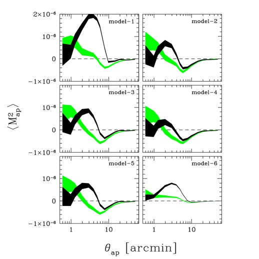
Figure 1: The $E$ (black area) and $B$-modes (light/green area) aperture mass statistics computed from the residual shapes of the stars after correcting using on of the six PSF models discussed in the text. The areas indicate the $1\sigma$ regions around the mean.

In the absence of more detailed information, Figure 1 provides a very useful way to choose which of the PSF correction models works best. The rational function (model 6) shows the smallest contamination on all scales. In particular the deviation from zero starts at a smaller scale than the other models. Figure 1 demonstrates there is still room left for an even better correction at small scales, but the lack of suitable stars makes this a very challenging issue.

Table 1: Different Point Spread Function parametric models used to correct the star anisotropy in the VIRMOS data. The table lists the basis of functions of the models. Model 6 is a rational function, the other models have $b_{lm}=0$.

model #	Correction Model
1	$(1,x,y,x^{2},xy,y^{2})$
2	$(1,x,y,x^{2},xy,y^{2},x^{3},y^{3},y^{4})$
3	$(1,x,y,x^{2},xy,y^{2},y^{3})$
4	$(1,x,y,x^{2},xy,y^{2},y^{3},y^{4},y^{5},x^{3},x^{4})$
5	$(1,x,y,x^{2},xy,y^{2},x^{3},y^{3})$
6	$(1,x,y,x^{2},xy,y^{2},y^{3},y^{4})/(x,y)$

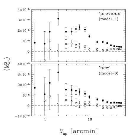
Figure 2: top panel: $E$ (filled points) and $B$ (open points) mode aperture mass measurements as measured from the previous analysis. It uses model-1 (see Table 1) to describe the PSF anisotropy with the wrong centroid estimate and no sigma clipping on the shape parameters of the selected stars. bottom panel: results using model 6 and the improved catalogues. Because of a different object selection in the new version, we ensured that we only used objects that are in common to produce this Figure. The new catalogue contains more galaxies.

These new insights in the correction for PSF anisotropy have led to a significant reduction in the level of systematics of the VIRMOS-Descart cosmic shear signal, as we will demonstrate below. Several other sources of the $B$ mode observed by Van Waerbeke et al. (2002) were identified as well. The systematics that have been corrected for in the revised analysis presented here are:

1. The small scale $B$ mode was generated by an imperfect PSF correction model as described above. As suggested in Hoekstra (2004) a proper correction for PSF anisotropy lowered the $E$ mode signal on these scales.

2. The large scale constant $B$ mode was caused by an imperfect calculation of the centroid of the objects. This problem was the most difficult to find because it was caused by a subtle inconsistency between the centroid estimate (based on SExtractor) and the shape calculation (based on IMCAT). On one of the VIRMOS fields (F10), SExtractor systematically computed a biased centroid which was the cause of the large scale bias in shape measurement generating a $B$ mode. This problem was cured by measuring the centroids using aperture filters instead of isophotal apertures.

3. The third important source of systematics arose from spurious ellipticies for some of the selected stars. Some of the stars survived the selection criteria based on a sigma clipping applied to their corrected ellipticity. It turned out that some stars passed this selection criteria, but their smear polarisability tensor was significantly different from the bulk of the stars (for a definition see Kaiser et al. 1995). This could happen when a star has a small very close companion which would contaminate the derivative of the profile much more than its ellipticity. The application of a $3-\sigma$ clipping to all of the star parameters, corrected ellipticity, smear polarisability and the stellar part of the preseeing shear polarisability remove all the remaining unwanted stars which contributed to the residual $B$ mode.

Figure 2 demonstrates how the results have changed from the early VIRMOS analysis (top panel) and the current analysis (bottom). The top panel shows clearly the small and large scale residual $B$ mode as measured before and a “bump” in the $E$ mode at $\sim 5$ arcminutes. The bottom panel shows the improvement after the main residual systematics have been corrected for. It also shows that the aperture mass is an effective statistic to identify and quantify residual systematics.

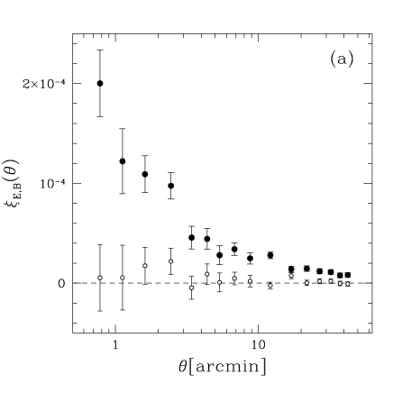
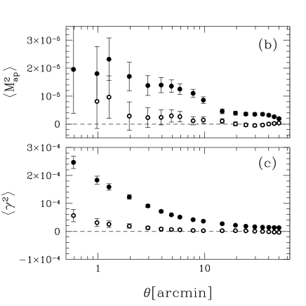
Figure 3: Panel (a): $E$ and $B$ mode shear correlation function (filled and open points, respectively) as measured from the VIRMOS-Descart data; panel (b): $E$ and $B$ mode measurements for the aperture mass statistic; panel (c): as before but now for the top-hat variance. For all three statistics we observe the signal is consistent with no $B$-mode on large scales, and a hint of minor contamination on small scales.

4.2 Residual systematics

The results of the new analysis of the VIRMOS-Descart are presented in Figure 3. To derive these measurements, all sources of systematics discussed in the previous section have been accounted for, and model 6 was used to characterize the spatial variation of the PSF anisotropy. Figure 3a shows the resulting ellipticity correlation function as a function of angular scale. The measurements are tabulated in Table 2. As explained in Section 2, in order to separate the signal into an $E$ and $B$ mode for the top-hat shear variance and shear correlation function, we have to define a zero-point for the $B$ mode. Based on the results for the aperture mass statistic (panel b) the correlation functions are scaled such that the mean $B$ mode is zero on scales $2-10^{\prime}$ according to the vanishing $B$ mode for the aperture mass at $\theta=10-50^{\prime}$. The error bars reflect only the statistical error bars. There is no cosmic variance on the $B$ mode, and consequently the statistical error is an unbiased estimate of the $B$ mode noise.

Panels (b) and (c) show the aperture mass $\langle M_{\rm ap}^{2}\rangle$ and the shear top-hat variance $\langle\gamma^{2}\rangle$, respectively. The measurements of both statistics are listed in Table 3. The small scale $\langle M_{\rm ap}^{2}\rangle$ $B$ mode is consistent with no signal (i.e., no systematics). However, one has to bear in mind that different PSF correction models produce fluctuations up to $10\%$ in the amplitude of the aperture mass below $1^{\prime}$. On the other hand, the aperture mass signal is robust against changes in the adopted PSF correction model for the range of scales $10-50^{\prime}$ which corresponds to a physical angular scale range of $2-10^{\prime}$. This means that the smallest scales in the aperture mass statistics give robust cosmological signal only if the PSF variation is properly removed.

The amount of residual systematics left in the signal due to imperfect PSF correction can be estimated from the correlation between the uncorrected stars and the corrected galaxies. Such an estimator was defined in Heymans (2003):

$$\xi_{\rm SYS}={\langle e^{\star}\gamma\rangle^{2}\over\langle e^{\star}e^{\star}\rangle}.$$ (15)

where $e^{\star}$ is the star ellipticity before PSF correction, and $\gamma$ is the shear estimate of the galaxies. $\xi_{\rm SYS}$ is renormalised by the star ellipticity correlation function $\langle e^{\star}e^{\star}\rangle$, which makes it directly comparable to the signal $\langle\gamma(r)\gamma(\theta+r)\rangle$, and not dependent on $|e^{\star}|$.

Figure 4 shows $\xi_{\rm SYS}$ for the VIRMOS data. The residual PSF contamination is consistent with no signal except maybe for one point around $\theta\simeq 22{\rm arcmin}$, which is at 2.4$\sigma$. It demonstrates that the anisotropy of the PSF has been almost completely removed. However, this plot provides no information about the accuracy of the isotropic PSF correction (the “pre-seeing” shear polarisability). As outlined in Hirata & Seljak (2003), the accuracy of the isotropic correction of the PSF is still somewhat uncertain, essentially because there is yet no direct way to obtain a perfect calibration of the shear amplitude to compensate for the PSF smearing. One should emphasize that Erben et al. (2001) and Bacon et al. (2001) used simulated images to demonstrate that the shape measurement method used in this paper (Kaiser et al. 1995) is accurate to $5\%$ or better at recovering the correct shear amplitude. The worst calibration was obtained for the most ellipticial galaxies. Hence, we expect an accuracy due to isotropic calibration smaller than $5\%$ in this study, which is still smaller than the statistical error. The PSF analysis technique based on reducing the $B$ mode amplitude shows how it is possible to control the PSF anisotropy correction, however the isotropic correction still has to be checked using simulated images.

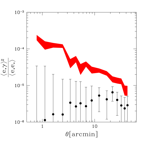
Figure 4: The shades (red) area corresponds to the $1\sigma$ area around the mean shear correlation function $\langle\gamma(r)\gamma(\theta+r)\rangle$ measured from the VIRMOS-Descart data. The points with error bars show the residual systematics correlation function $\xi_{\rm SYS}$ as defined in the text. The indicated error bars are those of the shear correlation function, and are displayed to show the level of systematics with respect to the $1-\sigma$ statistical error.

Table 2: $E$ and $B$ modes of the shear correlation function. The error is statistical only (see Section 6 for the covariance error).

$\theta$	$\xi_{E}$	$\xi_{B}$	$\delta\xi$
0.780000	0.000200166	5.43400e-06	3.33000e-05
1.12000	0.000122166	5.53400e-06	3.25000e-05
1.61000	0.000109166	1.74340e-05	1.85000e-05
2.45000	9.75660e-05	2.18340e-05	1.32000e-05
3.42000	4.56660e-05	-4.60600e-06	1.14000e-05
4.39000	4.43660e-05	9.03400e-06	1.03000e-05
5.37000	2.80660e-05	8.14000e-07	9.46000e-06
6.83000	3.40660e-05	4.73400e-06	6.29000e-06
8.79000	2.48660e-05	2.03400e-06	5.71000e-06
12.2000	2.79660e-05	-2.24600e-06	3.38000e-06
17.0800	1.39860e-05	7.53400e-06	2.98000e-06
21.9600	1.46060e-05	3.04000e-07	2.76000e-06
27.0100	1.18960e-05	1.93400e-06	2.51000e-06
32.3300	1.10960e-05	2.03400e-06	2.32000e-06
37.5400	7.80100e-06	-2.06000e-07	2.31000e-06
42.5400	8.22120e-06	-7.46000e-07	2.23000e-06

Table 3: Values of the aperture mass and shear top-hat variance as a function of scale. The $B$ mode is rescaled to zero for the later, and the error is statistical only.

$\theta$	$\langle M_{\rm ap}^{2}\rangle$	$\langle M_{\rm ap}^{2}\rangle_{\perp}$	$\delta\langle M_{\rm ap}^{2}\rangle$	$\langle\gamma_{E}^{2}\rangle$	$\langle\gamma_{B}^{2}\rangle$	$\delta\langle\gamma^{2}\rangle$
0.59	0.1956E-04	-.2560E-04	0.1571E-04	0.000246658	5.66021e-05	2.18700e-05
0.98	0.1806E-04	0.8109E-05	0.9666E-05	0.000183258	3.11921e-05	1.41900e-05
1.27	0.2318E-04	0.9647E-05	0.7599E-05	0.000158658	2.56821e-05	1.14700e-05
1.97	0.1703E-04	0.2864E-05	0.5083E-05	0.000122858	1.90721e-05	8.00500e-06
2.94	0.1378E-04	0.2319E-05	0.3512E-05	9.08879e-05	1.26021e-05	5.69900e-06
3.92	0.1395E-04	0.2413E-05	0.2704E-05	7.15379e-05	8.56213e-06	4.45700e-06
4.89	0.1357E-04	0.2952E-05	0.2217E-05	5.92279e-05	6.85213e-06	3.68800e-06
5.87	0.1250E-04	0.2675E-05	0.1884E-05	5.09079e-05	5.65212e-06	3.15500e-06
7.82	0.1100E-04	0.1198E-05	0.1465E-05	4.18679e-05	3.34212e-06	2.47200e-06
9.76	0.8562E-05	0.1469E-05	0.1210E-05	3.63379e-05	2.52213e-06	2.04900e-06
14.65	0.4570E-05	0.1084E-05	0.8642E-06	2.72479e-05	2.59212e-06	1.46700e-06
19.52	0.3899E-05	0.1008E-06	0.6924E-06	2.18579e-05	2.45213e-06	1.17100e-06
24.41	0.3594E-05	-.2831E-06	0.5858E-06	1.83569e-05	1.92213e-06	9.88100e-07
29.62	0.3503E-05	-.4899E-06	0.5065E-06	1.61539e-05	7.78125e-07	8.55300e-07
35.05	0.3537E-05	-.3382E-06	0.4477E-06	1.50329e-05	-3.31876e-07	7.56800e-07
40.05	0.3197E-05	0.4226E-07	0.4088E-06	1.43569e-05	-1.40988e-06	6.89600e-07
45.05	0.2635E-05	0.2219E-06	0.3804E-06	1.37509e-05	-2.50788e-06	6.38200e-07
49.95	0.1956E-05	0.3912E-06	0.3599E-06	1.30189e-05	-3.49488e-06	5.99200e-07

5 Parameter estimation

5.1 Likelihood calculation

Following Van Waerbeke et al. (2002), we investigate a four dimensional parameter space defined by the mean matter density $\Omega_{M}$, the normalisation of the power spectrum $\sigma_{8}$, the shape parameter $\Gamma$ and the redshift of the sources parameterized by $z_{s}$ (see Eq.(12)). We adopt a flat cosmology, unless stated otherwise. The default priors are taken to be $\Omega_{M}\in[0.1,1]$, $\sigma_{8}\in[0.5,1.3]$, $\Gamma\in[0.1,0.5]$ and $z_{s}\in[0.38,0.48]$. The latter corresponds to a mean redshift between $0.8$ and $1.0$, in agreement with Le Fèvre et al. (2004).

The data vector $\xi_{i}$ is the shear correlation function $\xi_{E}$ as a function of scale, as listed in Table 2. This table also shows that the residual systematic $\xi_{B}$ is negligible. If we take $m_{i}(\Omega_{M},\sigma_{8},\Gamma,z_{s})$ to be the model prediction, the likelihood function of the data is given by

$${\cal L}={1\over(2\pi)^{n}|{\bf C}|^{1/2}}\exp\left[(\xi_{i}-m_{i}){\bf C}^{-1}(\xi_{i}-m_{i})^{T}\right],$$ (16)

where $n=16$ is the number of angular scale bins and ${\bf C}$ is the $16\times 16$ covariance matrix,

$$C_{ij}=\langle(\xi_{i}-m_{i})^{T}(\xi_{j}-m_{j})\rangle.$$ (17)

${\bf C}$ can be decomposed as ${\bf C}={\bf C}_{n}+{\bf C}_{s}$, where ${\bf C}_{n}$ is the statistical noise and ${\bf C}_{s}$ the cosmic variance covariance matrix. ${\bf C}_{n}$ is diagonal and given in Table 2 (last columns). The matrix ${\bf C}_{s}$ is computed according to Schneider et al. (2002), assuming an effective survey area of $8.5$ square degrees, a number density of galaxies $n_{gal}=15{\rm\ per\ arcmin}^{2}$, and an intrinsic ellipticity dispersion $\sigma_{e}=0.44$. These numbers can be found in Van Waerbeke et al. (2002). The cosmic variance is computed assuming a Gaussian statistic, but as shown in Van Waerbeke et al. (2002), this is not an issue in our case: the non gaussian contribution appears only at small scale, where the noise is still dominated by the statistical error. We need a fiducial model to compute the matrix components, which is taken as the best fit model following the WMAP results (Spergel et al. 2003). It corresponds to the choice $\Omega_{M}=0.3$, $\Lambda=0.7$, $\sigma_{8}=0.85$, $\Gamma=0.21$ (the reduced Hubble constant is $h$=0.7). We take a mean source redshift for the fiducial model of $0.9$, which corresponds to $z_{s}=0.43$. Table 4 gives the full covariance matrix ${\bf C}$ used in this paper. The pure cosmic variance part of the matrix (${\bf C}_{s}$) can easily be extracted by subtracting the statistical noise contribution given in Table 2. The $B$ mode is calibrated by marginalizing around $B=0$ within the 1$\sigma$ interval.

Table 4: Full covariance matrix ${\bf C}$, as discussed in the text, Section 6. Units are $10^{-10}$. The scales $\theta_{i}$ correspond to those given in Table 2.

	$\theta_{1}$	$\theta_{2}$	$\theta_{3}$	$\theta_{4}$	$\theta_{5}$	$\theta_{6}$	$\theta_{7}$	$\theta_{8}$	$\theta_{9}$	$\theta_{10}$	$\theta_{11}$	$\theta_{12}$	$\theta_{13}$	$\theta_{14}$	$\theta_{15}$	$\theta_{16}$
$\theta_{1}$	14.48	2.15	1.85	1.55	1.33	1.20	1.10	1.01	0.92	0.80	0.70	0.62	0.56	0.49	0.44	0.40
$\theta_{2}$	2.16	13.57	1.87	1.56	1.34	1.20	1.10	1.01	0.92	0.81	0.70	0.62	0.56	0.49	0.44	0.40
$\theta_{3}$	1.86	1.88	5.57	1.57	1.35	1.21	1.11	1.01	0.92	0.81	0.70	0.62	0.56	0.49	0.44	0.40
$\theta_{4}$	1.56	1.57	1.58	3.46	1.38	1.22	1.12	1.02	0.92	0.81	0.70	0.62	0.56	0.49	0.44	0.40
$\theta_{5}$	1.34	1.35	1.36	1.38	2.78	1.25	1.15	1.04	0.92	0.81	0.70	0.62	0.56	0.49	0.44	0.40
$\theta_{6}$	1.21	1.21	1.21	1.23	1.26	2.41	1.16	1.04	0.93	0.81	0.70	0.62	0.56	0.49	0.44	0.40
$\theta_{7}$	1.10	1.10	1.11	1.12	1.15	1.17	2.14	1.05	0.93	0.81	0.70	0.61	0.56	0.49	0.44	0.40
$\theta_{8}$	1.01	1.01	1.03	1.03	1.04	1.04	1.05	1.50	0.94	0.81	0.69	0.62	0.56	0.49	0.44	0.40
$\theta_{9}$	0.92	0.92	0.92	0.93	0.92	0.93	0.93	0.95	1.32	0.82	0.70	0.62	0.56	0.49	0.44	0.40
$\theta_{0}$	0.80	0.80	0.81	0.81	0.81	0.81	0.81	0.81	0.82	0.96	0.70	0.62	0.55	0.48	0.44	0.40
$\theta_{11}$	0.70	0.70	0.70	0.70	0.70	0.70	0.70	0.69	0.70	0.71	0.82	0.62	0.55	0.51	0.44	0.41
$\theta_{12}$	0.62	0.62	0.62	0.62	0.62	0.62	0.62	0.62	0.63	0.62	0.62	0.72	0.55	0.48	0.44	0.39
$\theta_{13}$	0.56	0.56	0.56	0.56	0.56	0.56	0.56	0.56	0.56	0.56	0.55	0.55	0.62	0.49	0.44	0.39
$\theta_{14}$	0.49	0.49	0.49	0.49	0.49	0.49	0.49	0.50	0.50	0.49	0.51	0.48	0.49	0.56	0.44	0.39
$\theta_{15}$	0.44	0.44	0.44	0.44	0.44	0.44	0.44	0.44	0.44	0.44	0.44	0.44	0.44	0.44	0.50	0.39
$\theta_{16}$	0.40	0.40	0.40	0.40	0.40	0.40	0.40	0.40	0.40	0.40	0.41	0.39	0.40	0.40	0.40	0.46

The results of the maximum likelihood analysis are presented in Figure 5, which shows the constraints in the $\Omega_{M}$-$\sigma_{8}$ plan for the non-linear prediction schemes described in Smith et al. (2003). We note that we find similar results for the Peacock & Dodds (1996) model, although the best fit cosmologies differ somewhat (e.g., see Figure 6). We marginalised over $\Gamma\in[0.1,0.3]$ and $z_{s}\in[0.4,0.48]$, assuming a flat probability distribution in these intervals. For the Smith et al. (2003) model we find

$$\sigma_{8}=(0.83\pm 0.07)\left(\Omega_{m}\over 0.3\right)^{-0.49}.$$ (18)

For the Peacock & Dodds (1996) model we find a somewhat higher normalisation, given by

$$\sigma_{8}=(0.86\pm 0.08)\left(\Omega_{m}\over 0.3\right)^{-0.49}.$$ (19)

The difference between these two non-linear models corresponds to a 4% discrepancy, and it shows the limitation in the cosmic shear signal interpretation due to non-linear modeling. As the Smith et al. (2003) is the most recent, and more extensive analysis of the non-linear power spectrum, we prefer the results of this model. The updated results are also in excellent agreement with results obtained from the Red-sequence Cluster Survey (Hoekstra et al. 2003), who found $\sigma_{8}=0.86^{+0.04}_{-0.05}$ for $\Omega_{m}=0.3$. They are also in agreement with the revisited CTIO lensing survey (Jarvis & Jain 2004).

Figure 6 shows the probability distribution functions for $\sigma_{8}$ for the two models, adopting $\Omega_{m}=0.3$. Despite the different maximum likelihood shifts between the models, the curves are well fitted by a gaussian distribution as shown by the dashed line.

It is interesting to note that the new PSF anisotropy correction drops the resulting $\sigma_{8}$ only by 10% as compared to Van Waerbeke et al. (2001), much less than what would be expected from the change in amplitude in the lensing signal. However, in Van Waerbeke et al. (2001), the source redshift distribution was given by the model described in Wilson et al. (2001) (their figure 4), which turns out to give too much weight to high redshift galaxies compared to what we know about the VIRMOS galaxy sample today (Le Fèvre et al. 2003, 2004). . Hence the residual systematics in Van Waerbeke et al. (2001) were partly compensated by this biased redshift distribution model. For the present analysis we use more recent results from a comparison with photometric and spectroscopic redshifts (Le Fèvre et al. 2003, 2004). This changes the redshift distribution and significantly reduces the associated uncertainties.

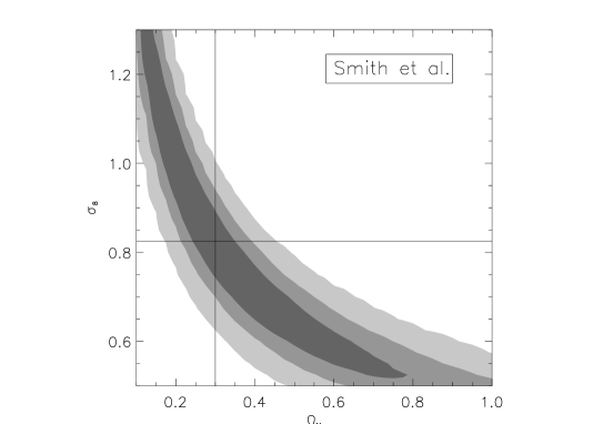
Figure 5: Constraints on $\sigma_{8}$ and $\Omega_{M}$ for a flat CDM Universe, adopting the non-linear prediction given by Smith et al. (2003). The contours correspond to the $0.68$, $0.95$ and $0.999$ confidence levels. The solid dark vertical line indicates $\Omega=0.3$ and the horizontal line indicates the maximum of the likelihood for $\sigma_{8}$ at $\Omega=0.3$. The models are marginalised over $\Gamma\in[0.1,0.3]$ and $z_{s}\in[0.4,0.48]$.

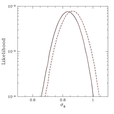
Figure 6: $\sigma_{8}$ probability distribution functions for $\Omega_{M}=0.3$. Dashed curve is for Peacock & Dodds (1996) (high normalisation), and the solid curve for Smith et al. (2003) (low normalisation). The superimposed dotted lines indicate a Gaussian fit to the likelihood function.

5.2 Combination with WMAP

Figure 5 indicates that a high density Universe $\Omega_{M}=1$ is excluded at the 2-$\sigma$ level. This result, however, depends on the prior used for the shape parameter $\Gamma\sim\Omega_{M}h$ (which is $\Gamma\in[0.1,0.3]$), and therefore on the Hubble constant (and the baryon abundance to a less extent). Using weak lensing data alone, it is still possible to accommodate $\Omega_{M}\simeq 1$, provided $\Gamma$ is at least as large as $0.5$, and we cannot exclude the high density ($\Omega_{M}>0.9$) alternative to the concordance model, proposed by Blanchard et al. (2003). The latter model only works if the Hubble constant is low ($\sim 0.5$, which is not in agreement with Freedman et al. (2001)) and if the Universe expansion rate is not accelerating as suggested by the type Ia supernovae results (Riess et al. 1998; Perlmutter et al. 1999).

From the cosmic shear point of view, such a model would require a low normalisation $\sigma_{8}\simeq 0.4$, because for higher values of $\Gamma$, the banana shape contour in the $\Omega_{M}-\sigma_{8}$ plane (Figure 5) is tilted clockwise. For example, the combination of $\Gamma=0.5$ and $\sigma_{8}=0.5$ is excluded at more than 3-$\sigma$. This is inconsistent with WMAP (Spergel et al. 2003) which gives $\sigma_{8}=0.9\pm 0.1$ for a flat and adiabatic Cold Dark Matter model assuming a power law primordial power spectrum.

Combined with our cosmic shear results, this leads to a rejection of the very low and high density universes, with a preferred value around $\Omega_{M}\simeq 0.3$, as indicated by Figure 7. This result also demonstrates that CMB and cosmic shear experiments are complementary, enabling one to break the $\Omega_{M}-\sigma_{8}$ degeneracy without external data sets (Contaldi et al. 2003; Tereno et al. 2004). Although one can modify the matter content of the Universe to try to account for a low $\sigma_{8}$ at high $\Omega_{M}$ (Blanchard et al. 2003), the next generation of weak lensing survey will certainly give an unambiguous constraint on $\sigma_{8}$ at low redshift regardless the value of $\Omega_{M}$.

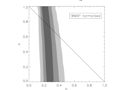
Figure 7: VIRMOS-Descart data constraints in the $\Lambda-\Omega_{M}$ plane. The models are normalised to the WMAP results ($\sigma_{8}=0.9\pm 0.1$), and we assumed the priors $\Gamma=[0.1,0.5]$ and $z_{s}=[0.4,0.48]$.

6 Conclusion

We have presented a revised analysis of the VIRMOS-Descart cosmic shear data, focussing on how to deal with residual systematics. The main result of this paper is a $10\%$ smaller mass power spectrum normalisation compared to our previous estimate. We find $\sigma_{8}=0.83\pm 0.07$ (for the preferred non-linear power spectrum as described by Smith et al. (2003)), which is at the 1-$\sigma$ bottom end of the measurement given in Van Waerbeke et al. (2002), where the systematics discussed in this study were still present. Our better understanding of systematics allows us to use weaker cosmic shear signal at higher angular scale and therefore to be less sensitive to unknown properties of the non-linear power spectrum.

In this work, various sources of systematics, which were previously ignored, were identified and the amplitude of the residual $B$ mode from the aperture mass was used to significantly improve the cosmological lensing signal. The choice of a better model to describe the spatial variation of PSF anisotropy at small scale proved to be critical for an unbiased measurement. We demonstrated that small differences between correction schemes can have a significant impact on the small scale signal. Fortunately, the residual systematics in the aperture mass of the stars provide an unambiguous method to test for residual systematics by selecting the least biased model.

On large scales, a few outliers in the star catalogue used to correct for the effects of the PSF can introduce a bias even if their ellipticities appear reasonable. It is therefore important to reject spurious stars not only from their corrected ellipticity, but using extended criteria such as the smear polarisability and the preseeing shear polarisability. We also found that a large angular scale bias can be introduced from the use of galaxy centroids based on isophotal cuts.

There is a fundamental limit to the accuracy of the correction at small scales, which is determined by the sampling of the PSF variation across the CCDs. Further high precision cosmic shear studies will require the observation of dense star fields to improve the correction (see Hoekstra 2004). Fortunately, the large scale signal ($>10^{\prime}$) appears unaffected by the choice of the PSF anisotropy model.

The use of the shear correlation function is much less sensitive to systematics than the shear top-hat variance or even the aperture mass variance. This is most critical for the aperture mass which is sensitive to very small scales. On the other hand, the aperture mass $B$ mode is a crucial test of the residual systematics, which has to be used to calibrate the PSF correction and the $B$ mode of the shear correlation function.

The prediction of the non-linear power spectrum results in values for $\sigma_{8}$ that differ by a few percent for different models. The model presented by Smith et al. (2003) always gives a smaller normalisation than Peacock & Dodds (1996). Currently, the former provides the preferred model. We also note that these differences are not yet an important issue for surveys of the size we considered here. However, it will be a challenging task for the forthcoming lensing surveys to improve the non-linear predictions to the required level of precision.

It is still possible to accommodate a large value for $\Omega_{m}$ from cosmic shear measurements alone. However, the combination of the cosmic shear signal with measurements of the Cosmic Microwave Background provides strong evidence for a low density universe without adding external data sets. To derive these conclusions we do have to assume a Cold Dark Matter scenario with a primordial power law power spectrum. Such assumptions can be relaxed with the next generations of lensing surveys.