ANIS: High Energy Neutrino Generator for Neutrino Telescopes

Abstract

We present the high-energy neutrino Monte Carlo event generator ANIS (All Neutrino Interaction Simulation). The program provides a detailed and flexible neutrino event simulation for high-energy neutrino detectors, such as AMANDA, ANTARES or ICECUBE. It generates neutrinos of any flavor according to a specified flux and propagates them through the Earth. In a final step neutrino interactions are simulated within a specified volume. All relevant standard model processes are implemented. We discuss strengths and limitations of the program.

Program Summary
Title of program: ANIS
Program is obtainable from: http://www-zeuthen.desy.de/nuastro/anis/anis.html
Computer on which the program has been thoroughly tested: Intel-Pentium based Personal Computers
Operating system: Linux
Programming language used: C++
Memory required to execute: 13 megabyte
Number of lines in distributed program (version 1.8): 3300
Libraries used by ANIS: HepMC [1], CLHEP vector package [2]
Nature of physical problem: Monte Carlo neutrino event generator for high-energy neutrino telescopes
Method of solution: Neutrino events are first sampled according a specified flux, then propagated through the Earth and finally are allowed to interact inside a detection volume.
Restrictions of the program: Neutrino energies range from 10 GeV to $10^{12}$ GeV.
Typical running time: $10^{4}$ events require typically a 1-GHz CPU time of about 300 s

1 Introduction

The first generation of open water/ice Cherenkov neutrino telescopes take data (AMANDA [3], BAIKAL [4]) or are under construction (ANTARES [5], NESTOR [6]) while the second generation projects such as IceCube [7] are already in the planning phase. Such devices aim at detection of cosmic high-energy neutrinos. Cherenkov photons from charged particles produced in neutrino interactions near or inside the detector are used to identify neutrinos. Because of their large volume and coarse granularity, the energy threshold of these open instruments is typically between 10 GeV and 100 GeV and therefore high when compared to that of closed underground Cherenkov detectors, such as SuperKamiokande and SNO. The flux of neutrinos produced by interactions of cosmic rays in the atmosphere (so called atmospheric neutrinos) falls steeply with energy ($\frac{{\rm d}N}{{\rm d}E_{\nu}}\propto E_{\nu}^{-3.7}$). Hence the event rate due to atmospheric neutrinos is largest near the detection threshold energy. This is different for astrophysical neutrino fluxes which generally are assumed to have harder spectra. Potential sources for astrophysical neutrinos could be astrophysical objects such as Active Galactic Nuclei (AGN), Gamma Ray Bursts (GRBs) or heavy relic particles, such as produced e.g. in decays of Topological Defects (TD). The relevant range of neutrino energies from the more conventional sources such as AGN and GRBs range from $10^{3}$ GeV, to $10^{9}$ GeV, energies while the range of neutrinos expected from TD models extends up to $\sim 10^{15}$ GeV energies.

Apart from the desired astrophysical neutrinos and atmospheric neutrinos, high-energy neutrino telescopes detect muons produced in cosmic ray interaction in the atmosphere (so called atmospheric muons). Due to the low interaction probability of neutrinos, the trigger rates due to atmospheric muons is generally orders of magnitude higher than that of atmospheric neutrinos. Hence a large number of search strategies are used, for example using the Earth as a shield and selecting only events with horizontal and upward going directions.

In the analysis of the data of neutrino telescopes, Monte Carlo (MC) simulations play a decisive role in designing and testing event reconstructions and filters, determining filter efficiencies and interpreting the results. Various programs exist for event simulations. For example, atmospheric muons can conveniently be simulated with the air-shower program CORSIKA [8]. The generated muons are further propagated through the overburden consisting of water or ice using muon propagation programs such as MMC [9], MUM [10] or PROPMU [11]. In a final step the detector response needs to be simulated using detector specific programs. Programs for simulating neutrino events are known to exist within various collaborations, however, to our knowledge they are not publicly available. In particular most programs simulate only some specific classes of events (for example $\nu_{\mu}$ reactions) in a limited range of energies.

Here, we present the program ANIS for simulating neutrino events of all flavors in a wide range of energies. ANIS is a Monte Carlo event generator, which prepares neutrinos, propagates them through the Earth and in a last step simulates a neutrino interaction within a specified volume around the detector. The aim of the program is to provide a tool for precise simulation of neutrino events of all flavors in the energy range addressed by high-energy neutrino telescopes. The program has been designed to fulfill the requirements for analysis of AMANDA data, and could hence be of use for other neutrino telescopes.

An application of ANIS was demonstrated in [12], where the expected rates for $\nu_{e}$ events as calculated with ANIS were presented. The source code as well as further documentation can be obtained from the project web site: http://www-zeuthen.desy.de/nuastro/anis/anis.html.

The paper is organized as follows. First a general description of the program is given in Section 2. The implemented neutrino interaction processes are shortly discussed in Section 3. The possibility to add a new (non-standard model) interaction process to ANIS is demonstrated there by an example. In Sections 4 and 5 the role of tau leptons and how neutrino propagation is simulated in ANIS are discussed. A description of the treatment of the final neutrino interactions inside the detection volume follows in Section 6. Additional information relevant for potential users is given in the appendix.

2 Description of the program

ANIS is written in C++ and uses the vector package of the CLHEP library [2] as well as the HepMC Monte Carlo event record [1]. The event record holds all interaction vertices with their respective incoming and outgoing particles. The currently implemented interaction channels include charged current (CC) and neutral current (NC) interactions as well as resonant $W^{-}$ production: $\bar{\nu}_{e}e^{-}\rightarrow W^{-}\rightarrow anything$.

Primary neutrinos are randomly generated on the surface of the Earth. Currently only power-law energy spectra $\phi_{\nu}(E)\propto E^{-\alpha}$ are implemented, however the code is flexible enough to allow its extension to arbitrary neutrino spectra.

ANIS propagates neutrinos in small steps towards the detector. In interactions with matter they are either absorbed (CC-case) or regenerated at lower energies (NC-case). In the special case of CC $\nu_{\tau}$ interaction, a short-living $\tau$-lepton is produced. It propagates in matter, thereby loosing part of its energy, and finally decays giving rise to a secondary $\nu_{\tau}$ and, in $\sim 17~{}\%$ of the cases, to secondary $\nu_{\mu}$ or $\nu_{e}$. The density profile of the Earth used for neutrino propagation is chosen according to the Preliminary Earth Model [13].

Once the detection volume is reached, a final vertex is generated along the neutrino trajectory within the detection volume. In the case of a CC $\nu_{\mu}N$-interaction, ANIS correctly simulates the muon scattering angle.

Along with the full event, four weights are stored: a normalization constant, a weight proportional to the total interaction probability of the neutrino as well as two weights corresponding to the atmospheric flux of electron and muon neutrinos [14].

Event rates for atmospheric and various extraterrestrial neutrino spectra are obtained by applying the appropriate weights to the events. This last step can conveniently be done by a user defined energy dependent weight function applied within analysis programs as e.g. PAW [15] and ROOT [16]. Applications of the weights are further discussed in appendix D.

There are currently two output formats implemented: i) the AMANDA specific event format f2000 [17] and ii) the HepMC ascii format [1].

3 Neutrino cross sections

At $E_{\nu}\lesssim 1\times 10^{6}$ GeV, deep inelastic $\nu N$-cross-sections may be successfully described in the framework of pQCD. Parameterization of the $\nu N$ structure functions, $F_{i}^{\nu N}(x,Q^{2})$, may be chosen e.g. according to CTEQ5 [18]. Here, $-Q^{2}=q^{2}$ is the invariant momentum transfer, with the 4-momentum $q=k_{\nu}-p_{l}$ given by the difference in momenta between the incoming neutrino and outgoing lepton. The ”Bjorken” variable $x$ is given by $x=Q^{2}/(2M_{N}(E_{\nu}-E_{l}))$ where $E_{\nu}$ and $E_{l}$ are the energies of the incoming neutrino and outgoing lepton.

At higher energies cross-sections are dominated by scattering off sea-quarks with small $x$. The unknown behavior of the structure functions at $x\lower 3.01385pt\hbox{$\;\stackrel{{\scriptstyle\textstyle<}}{{\sim}}\;$}10^{-6}$ makes the calculations model dependent. The uncertainty in extrapolations of $F_{i}^{\nu N}(x,Q^{2})$ to small $x$ and large $Q^{2}$ influences the expected cross-sections at high energies. Two options are presently included in ANIS: i) the smooth both with respect to $x$ and to $Q^{2}$ power-law extrapolation of the pQCD CTEQ5 parameterization to small $x$ and large $Q^{2}$, and ii) hard pomeron [19] enhanced extrapolation [20]. The cross-sections of the first case, denoted in the Fig. 1a as pQCD, practically coincide with [21], while the second model (HP, dash-dotted curves) predicts approximately $2$ times higher cross-sections at $E_{\nu}=1\times 10^{12}$ GeV.

A kinematically important variable is $y=1-\frac{E_{l}}{E_{\nu}}$, which characterizes the energy transfer to the outgoing lepton and to the final hadronic state. The $y$-distributions, normalized to the corresponding cross-sections, are plotted in Fig. 1b; the solid and dashed curves stand for CC and NC $\nu N$-interactions, respectively. The scattering angle, $\theta$, between incoming neutrino and outgoing lepton is given by

$$\cos\theta=1-\frac{xy}{1-y}\cdot\frac{m_{\rm N}}{E_{\nu}}.$$

The used cross-section data for CC- and NC-reactions are taken from pre-calculated tables. The total cross-section is obtained through interpolation between energy bins. A final state can be represented by the pair of $x$ and $y$. Large sets of $x$ and $y$ have been generated for different energies and are stored in data tables. During generation of neutrino events such pairs are randomly drawn from the tables. The use of pre-calculated tables makes the program fast and independent of other packages.

Figure 1: a) $\nu N$- and resonance $\bar{\nu}_{e}e^{-}$-cross-sections  and b) normalized $y$-distributions.

Since $m_{e}\ll m_{N}$, at high energies practically all $\nu e^{-}$-cross-sections are negligibly small, with the exception of resonant $W^{-}$ production $\bar{\nu}_{e}e^{-}\rightarrow W^{-}\rightarrow anything$ at $E_{\bar{\nu}_{e}}\approx 6.3\cdot 10^{6}$ GeV (the so called Glashow resonance, [22]) (see Fig. 1a). This process is also included in ANIS.

ANIS was designed such that new cross-sections and processes can be added at a later stage. Assuming for example, one would like to allow microscopic black hole production [23] one has to derive a new (C++) class for this process and provide the relevant member functions:

class SigmaBH : public Sigma {
   public:
     double GetSigma(const GenParticle* neutrino, double material[]);
     void FillVertex(GenVertex* vertex, double material[]);
}

GetSigma returns the cross section, and the function FillVertex inserts the final state. By adding this new process to the list of know processes, it will be included during simulation. Thereby all particles produced in the final states are written to the event record and in case of neutrinos are further propagated. In this way, any potential implications of non-standard model physics can easily be tested.

Already implemented SM processes can be modified even without modification of the code, simply by replacement of the cross-section data tables obtained using other programs.

4 Treatment of tau leptons

Tau leptons can be produced in CC $\nu_{\tau}N$-reactions and in resonance $\bar{\nu}_{e}e^{-}\rightarrow W^{-}\rightarrow\bar{\nu}_{\tau}\tau^{-}$ scattering. The average tau decay length is $l_{\tau}=49~{}{\rm m}\times(E_{\tau}/{\rm PeV})$. For energies larger than $E_{\tau}\sim 10^{8}\rm GeV$, the energy loss during propagation has to be taken into account, leading to a slower growth of the decay length. In the current version of the program, the stochastic effects in the energy loss rate are neglected. The energy loss rate is assumed to be continuous:

$$\frac{{\rm d}E_{\tau}}{{\rm d}X}=\alpha+\beta(E)E_{\tau},$$ (1)

with $\beta=(1.508+6.3\cdot(E/10^{9}~{}{\rm GeV})^{0.2})\cdot 10^{-7}{\rm cm^{2}/g}$ [24].

In contrast to muon propagation, neglecting stochastic energy losses does not alter the average $\tau$ range significantly [25]. At energies of $E_{\tau}\sim 10^{8}$ GeV, the continuous case is essentially indistinguishable from the stochastic case and at energies around $E_{\tau}\sim 10^{11}$ GeV the difference between the two cases is only a few percent. The reason, next to the energetic tau decay, is that in case of taus (hard) bremsstrahlung is suppressed while (softer) nuclear interactions dominate.

In ANIS, the tau is propagated in small steps of energy. Once the age in the tau rest-frame exceeds the previously determined lifetime the tau decay routines are called.

The tau decay is simulated with the help of TAUOLA [26]. Instead of linking directly to TAUOLA, we have created tables of final states, consisting of the fractional energy: hadronic ($\pi^{\pm},K,..$), electro-magnetic (e, $\pi^{0}$ and $\gamma$), muons, and the various neutrino flavors. Thereby we have assumed left-handed polarization of the tau leptons, which is a good approximation for neutrino interactions, if $E_{\tau}/m_{\tau}\gg 1$. The tau decay products are added to the event record and in case of neutrinos are further propagated.

5 Neutrino Propagation

Neutrinos are generated at the surface of the Earth and then propagated to the detector. They are assumed to travel along straight trajectories, neglecting the small angle neutrino scattering. This is a good approximation, since at energies below $10^{5}$ GeV when the average deflection angle (for example through NC reactions) becomes larger $0.1^{\circ}$, the neutrino interaction probability in the Earth is small. A deflection angle of $0.1^{\circ}$ is below the current instrumental resolution of existing or planned neutrino telescopes. The density profile of the Earth is chosen according to the Preliminary Earth Model [13]. Neutrinos are propagated in small steps through the Earth and in case of an interaction one of the active interaction channels is chosen according the inclusive cross-section. Its final state member function is invoked, which adds the final state of the interaction to the event record. Naturally, all propagation effects such as neutrino absorption, $\nu_{\tau}\rightarrow\tau\rightarrow\nu_{\tau}$ regeneration, regeneration in NC interactions as well as possible neutrino production in the resonant scattering of electrons (e.g., $\bar{\nu}_{e}\rightarrow W^{-}\rightarrow\nu_{e,\mu,\tau}$) are included.

6 Detection volume and final vertex

The size of the detection volume needs to be specified in the steering file. The shape of the volume is a cylinder with its $z$-axis parallel to the neutrino directions. Since open water/ice Cherenkov detectors have a sensitivity to events with vertices outside their fiducial volumes, the size of the cylinder should be chosen appropriately. In particular due to the potentially long range of muon and tau leptons, the final cylinder should extend to the direction of the neutrino origin. As an alternative, one can choose a cylinder with a variable length which adjusts to the energy-dependent maximally possible muon and tau range. The latter allows a more efficient simulation.

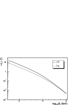
Figure 2: Average angle $\theta$ between the incoming neutrino and the outgoing muon in a CC reaction as a function of the neutrino energy.

Neutrinos reaching the detection volume are forced to interact within this volume. The interaction probability is stored in the event record. Two options are implemented: i) all events are written to disk – in order to obtain a physical spectrum, one needs to weight all events with their interaction probability, and ii) events are sampled according their interaction probability – the events are sampled using an acceptance-rejection method, where the selection criteria are determined at run time during initialization.

The final state depends on the flavor of the interacting neutrino, the type of the reaction as well as on the variables $x$ and $y$ of the interaction. Since Cherenkov neutrino telescopes cannot distinguish the different types of hadrons, the hadronization of the final state is omitted and all hadronic energy is written out as pions. Since neutrino telescopes have a muon angular resolution of $\mathcal{O}(1^{\circ}$), the scattering angle between incoming neutrino and outgoing muon needs to be taken into account. Fig. 2 shows the average scattering angle for neutrinos and anti-neutrinos as obtained with ANIS.

All muons of the final state have to be further propagated using dedicated muon propagations programs (such as MMC or MUM), before the events are passed to the detector simulation.

7 Conclusion

A new program for the simulation of neutrino induced events for high-energy neutrino telescopes is presented. The program fulfills current requirements for data analysis of neutrino telescopes, and is designed flexible such that new processes could be added in the future. The current version of ANIS includes all relevant SM neutrino interaction processes. The energies for which cross-section data is provided ranges from 10 GeV to $10^{12}$ GeV.

Acknowledgments

We acknowledge the contributions of Tonio Hauschild, suggestions and feedback from Stephan Hundertmark, as well as discussions with Gary Hill.

Appendix A Organization of the Program

The ANIS source code consists of several files in two directories: anis/ and sigma/. The first directory contains the part of the code related to the simulation of events, while the latter contains the part of the code related to interaction and decay of particles.

anis/
anis.cc – the main file of the program which calls the main processes.
Steer.cc – the steering file format.
AnisEvent.cc – the ANIS event record definition.
FluxDriver.cc – contains classes for simulating neutrino fluxes.
NeutrTraject.cc – contains classes for calculating neutrino trajectories.
Propagation.cc – contains classes related to the propagation of neutrinos through the Earth to the detector.
FinalVolume.cc – contains classes related to the final detection volume.
 FinalVertex.cc – classes for sampling the vertex within the final volume.
Earth.cc – contains information on the Earth density profile.
AnisIO.cc – definition of various output streams. (see also AnisEvent.cc).

sigma/
Sigma.cc – the virtual base class for all interaction processes.
SigmaSM.cc – all Standard Model processes.
SigmaTotal.cc – the container class holding all activated processes.
ProcessManager.cc – controls the active processes for the neutrino flavors and target materials.
Decay.cc – contains all decay classes.
Table.cc – contains various utility classes for reading the data tables.

Next we describe the most relevant classes and member functions:

class FluxDriver
void Inject (AnisEvent *evt)
- This method inserts the initial neutrino into the event record. The position of the neutrino origin is chosen on the Earth surface, such that the straight trajectory of the neutrino intersects the final detection volume.

class Propagate
void ThroughEarth (AnisEvent *evt)
- this method propagates all neutrinos in the event record up to the backside of the the final detection volume.

class SigmaTotal
double GetSigma (HepMC::GenParticle *nuin, double material[])
void FillVertex (HepMC::GenVertex *vtx, double material[])
- The GetSigma member function returns the total cross-section for a given neutrino and material (in the current version of the code isospin invariance is assumed: all interaction material contains equal numbers of neutrons, protons and electrons). The FillVertex member function samples an interaction type from the list of possible processes and fills the vertex record with corresponding outgoing particles.

class ParticleDecay
void AddVertex (HepMC::GenParticle *parent, AnisEvent *evt)
- this method inserts a decay vertex for the incoming parent particle into the event record. So far the only unstable particle implemented is the tau-lepton.

class FinalVertex
void ThrowVertex (AnisEvent *evt)
- this method inserts a final neutrino interaction (vertex) located within the final detection volume into the event record. The interacting neutrino is chosen (with a probability proportional to the its interaction probability) from all neutrinos reaching the final detection volume.

Further there is the control class Steer, which holds the run parameter of ANIS as well as the ProcessManager which controls the list of available interaction processes.

Further documentation of the code can be found on the project web site: http://www-zeuthen.desy.de/nuastro/anis/anis.html.

Appendix B The steering file

The program ANIS reads a steering file called ”steer.dat”. In case a file name is given in the command line, this file is taken as the steering file. The steering file contains all run specific information. Here is an example:

# The flux information
f p 1 1e2 1e4 -1. 1. 12
# The geometry information (volume is cylinder)
g c 300. 300. 300. 1.7e3 1
# The run information
r 100 1 1 2123421
# The cross-section processes and data.
s CC cteq5/cteq5_cc_nu.data cteq5/final_cteq5_cc_nu.data 101010 110
s CC cteq5/cteq5_cc_nubar.data cteq5/final_cteq5_cc_nubar.data 10101 110
s NC cteq5/cteq5_nc_nu.data cteq5/final_cteq5_nc_nu.data 101010 110
s NC cteq5/cteq5_nc_nubar.data cteq5/final_cteq5_nc_nubar.data 10101 110
s GR dummy dummy 10000 1
# the data directory
d ../data

Lines starting with a letter: s,f,g,r,d specify a program command line. Lines starting with # are for comments only.

• (flux): The f must be followed by a parameter specifying the spectrum type (p for power law, this is so far the only implemented one), the spectral index, the minimal neutrino energy, the maximal neutrino energy (in GeV), the minimal cosine of the zenith angle of the neutrino direction, and the maximal allowed cosine of the zenith angle. The last number indicates the neutrino type with the following possibilities: $12(=\nu_{e}+\bar{\nu}_{e})$, $14(=\nu_{\mu}+\bar{\nu}_{\mu}$), $16(=\nu_{\tau}+\bar{\nu}_{\tau}$).

• (geometry): The g is followed by the type of the final volume (c stands for cylinder, which is the only one implemented so far), the radius (in meter) and the +/- height of the volume. The height is given by two numbers, the first is the positive height (target region), and the second is the height in the detector region. The next element is the depth of the detector from the surface (in meter). The final number is optional: if set to 1, a geometry optimization is invoked: if the lepton range is larger than the specified volume, the volume is adjusted to the maximal lepton range. So far this option is implemented only for muon-neutrino. If the number is missing or set to 0, then no re-adjustment is made.

• (run parameter): The r is followed by the number of events to be simulated and the output format (1=HepMC,2=f2000). The third value indicates if weighted (1) or unweighted (0) events should be simulated. The last number is an optional seed for the generator. If no seed is present, the system time is used to seed the random number generator.

• (sigma): The information following the s is the type of the process (CC: charged current, NC: neutral current, GR: Glashow resonance) the file containing the cross-section data, the file containing the final state data, the active neutrino bit mask. ($\nu_{e}\bar{\nu}_{e}\nu_{\mu}\bar{\nu}_{\mu}\nu_{\tau}\bar{\nu}_{\tau}$, 101010 means all neutrinos, 10101 means all anti-neutrinos and 10000 means only electron anti neutrinos), and the active target material bit mask (110 means protons and neutrons, 1 means electrons).

• (data directory) this is the path to the data directory, containing the cross section, tau decay and neutrino flux data.

Figure 3: The geometry: the coordinate system is anchored at the detector center, with the z-axis pointing away from the Earth center. The cylinder represents the final volume, in which potentially detectable neutrino interactions are simulated. Its size is adjustable through the steering file.

Appendix C Output

Here only the HepMC event output format is discussed. An example for a neutrino event as generated with ANIS is shown below. It is the first of 1000 events generated with the steering file described above.

GenEvent: #1 ID=1 SignalProcessGenVertex Barcode: 0
Current Memory Usage: 1 events, 2 vertices, 3 particles.
Entries this event: 2 vertices, 3 particles.
RndmState(0)=
Wgts(4)=1.20431e-06 5.16006e+17 4.0188e-11 1.21211e-09
EventScale -1 GeV alphaQCD=-1 alphaQED=-1
GenParticle Legend
Barcode PDG ID ( Px, Py, Pz, E ) Stat DecayVtx
$\_\_\_\_\_\_\_\_\_\_\_\_\_\_\_\_\_\_\_\_\_\_\_\_\_\_\_\_\_\_\_\_\_\_\_\_\_\_\_\_\_\_\_\_\_\_\_\_\_\_\_\_\_\_\_\_\_\_\_\_\_\_\_\_\_\_\_\_\_\_\_\_\_\_\_\_\_\_\_\_\_\_\_\_\_\_\_\_\_\_$
VVertex: -1 ID: 1 (X,cT)=+5.37e+06,+1.26e+06,-2.98e+06,+0.00e+00
Wgts(1)=0
O: 1 10001 12 -4.32e+03,-1.01e+03,+2.40e+03,+5.05e+03 1 -2
Vertex: -2 ID: 0 (X,cT)=-3.50e+02,-7.01e+01,-8.75e+01,+0.00e+00
I: 1 10001 12 -4.32e+03,-1.01e+03,+2.40e+03,+5.05e+03 1 -2
O: 2 10002 11 -1.28e+03,-3.00e+02,+7.09e+02,+1.49e+03 1 (nil)
10003 211 -3.05e+03,-7.15e+02,+1.69e+03,+3.56e+03 1 (nil)
$\_\_\_\_\_\_\_\_\_\_\_\_\_\_\_\_\_\_\_\_\_\_\_\_\_\_\_\_\_\_\_\_\_\_\_\_\_\_\_\_\_\_\_\_\_\_\_\_\_\_\_\_\_\_\_\_\_\_\_\_\_\_\_\_\_\_\_\_\_\_\_\_\_\_\_\_\_\_\_\_\_\_\_\_\_\_\_\_\_\_$

Events consist of a list of vertices with attached incoming and outgoing particles as well as a list of weight. For a description of how to access events, vertex, particles and weights we refer to the HepMC documentation [1].

• All vertex positions are relative to the detector center (in units of meters). The orientation is such that $z$ axis is pointing upwards.

• The particle identification numbers follow the Particle Data Group scheme. Energy and momentum are given in units of GeV.

• Events have four weights attached: the interaction probability in the final volume ($P_{\rm int}$), a normalization constant ($N$) and two weights ($R_{\rm atm}^{\nu_{e}}$ and $R_{\rm atm}^{\nu_{\mu}}$) corresponding to the atmospheric neutrino flux for $\nu_{e}$ and $\nu_{\mu}$ [14].

Appendix D Using ANIS weights

To obtain physical distributions of variables (such as neutrino energy or flavor at the detector) from ANIS events, one can conveniently use the weights described in appendix C.

If events are generated according a spectral index $\gamma$ the application of an event weight $N\cdot P_{\rm int}$ will result in a simulated flux

$$\Phi(E)=(E/{\rm GeV})^{-\gamma}[\rm GeV^{-1}s^{-1}sr^{-1}cm^{-2}].$$

The normalization is chosen such that $N\cdot\sum\limits_{i=1}^{N_{\rm event}}P_{{\rm int},i}$ results in the total number of events per year in the specified volume. Other spectra can be obtained by applying additional weight factors. (For example, to obtain a flux with spectral index $\gamma^{\prime}$, the additional multiplicative weight should be $E^{\gamma-\gamma^{\prime}}$).

In case one is interested in an atmospheric neutrino spectrum, each event should be weighted according a weight $N\cdot P_{\rm int}\cdot R_{\rm atm}$, where the flux weight $R_{\rm atm}$ (which is provided by ANIS) should be chosen according to the simulated neutrino flavor. Again, the normalization of the resulting distribution corresponds to events per year in the specified volume.

Accounting neutrino oscillations of atmospheric neutrinos can be done using weighting functions. Assuming one is interested in muon neutrinos, and $P_{\nu_{e}\rightarrow\nu_{\mu}}$ is the energy and direction dependent probability for electron neutrinos to appear at the detector site as muon neutrinos, while $P_{\nu_{\mu}\rightarrow\nu_{\mu}}$ is the probability of the initial muon neutrino to be detected as muon neutrino. The corresponding weight for each event is then: $N\cdot P_{\rm int}\cdot(P_{\ \nu_{\mu}\rightarrow\nu_{\mu}}\cdot R_{\rm atm}^{\nu_{\mu}}+P_{\ \nu_{e}\rightarrow\nu_{\mu}}\cdot R_{\rm atm}^{\nu_{e}})$.

References

- [1] M. Dobbs and J. B. Hansen, Comput. Phys. Commun. 134 (2001) 41.
- [2] http://wwwinfo.cern.ch/asd/lhc++/clhep
-
[3]
E. Andres et al., Astropart. Phys. 13 (2000) 1;
see also http://www.amanda.uci.edu. - [4] V. Balkanov et al., Astropart. Phys. 14 (2000) 61.
- [5] U. F. Katz et al. arXiv:astro-ph/0310736; see also http://antares.in2p3.fr.
-
[6]
S. E. Tzamarias,
Nucl. Instrum. Meth. A 502 (2003) 150;
see also http://www.nestor.org.gr -
[7]
J. Ahrens et al., Astropart. Phys. 20 (2004) 507;
see also http://icecube.wisc.edu/ -
[8]
D. Heck et al., FZKA 6019. (1993);
see also http://www-ik3.fzk.de/heck/corsika - [9] D. Chirkin and W. Rhode, Proc. 27th Int. Cosmic Ray Conf. (ICRC 2001), Hamburg, Germany (2001).
- [10] I. A. Sokalski, E. V. Bugaev and S. I. Klimushin, Phys. Rev. D 64 (2001) 074015.
- [11] P. Lipari and T. Stanev, Phys. Rev. D 44 (1991) 3543.
- [12] M. Kowalski and A. Gazizov, Proc. Int. Cosmic Ray Conf. p. 1459, Tsukuba, Japan (2003).
- [13] see Ref. [83] in R. Gandhi et al., Astropart. Phys. 5 (1996) 81.
- [14] P. Lipari, Astropart. Phys. 1 (1993) 195.
-
[15]
PAW – Physics Analysis Workstation; User’s Guide,
ftp://asisftp.cern.ch/cernlib/doc/ps.dir/paw.ps.gz -
[16]
ROOT - An Object-Oriented Data Analysis Framework,
see http://root.cern.ch/ - [17] http://www-zeuthen.desy.de/nuastro/software/siegmund/f2000.ps.gz
-
[18]
CTEQ collab.: H. L. La et al. hep-ph/9903282;
http://www.phys.psu.edu/cteq/ - [19] A. Donnachie and P. V. Landshoff, Phys. Lett. 437B (1998) 408.
- [20] A. Z. Gazizov, S. I. Yanush Phys. Rev. D 39 (2002) 941.
- [21] R. Gandhi et al. Phys. Rev. D 58 (1998) 093009.
-
[22]
S. L. Glashow, Phys. Rev. 118 (1960) 316;
V. S. Berezinsky and A. Z. Gazizov, JETP Lett. 25 (1977) 276. -
[23]
S. Dimopoulos and G. Landsberg, Phys. Rev. Lett. 87
(2001) 161602;
S. B. Giddings and S. Thomas, Phys. Rev. D 65 (2002) 056010;
M. Kowalski, A. Ringwald and H. Tu, Phys. Lett. B 529 (2002) 1. - [24] S. I. Dutta, M. H. Reno, I. Sarcevic and D. Seckel, Phys. Rev. D 63 (2001) 094020.
-
[25]
D. Chirkin and W. Rhode, in preparation;
see also http://area51.berkeley.edu/manuscripts/20040303xx-muon.pdf. - [26] S. Jadach et al., Comput. Phys. Commun. 76 (1993) 361.