How Accurately can Suborbital Experiments Measure the CMB?

Abstract

Great efforts are currently being channeled into ground- and balloon-based CMB experiments, mainly to explore anisotropy on small angular scales and polarization. To optimize instrumental design and assess experimental prospects, it is important to understand in detail the atmosphere-related systematic errors that limit the science achievable with new suborbital instruments. For this purpose, we spatially compare the 648 square degree ground- and balloon-based QMASK map with the atmosphere-free WMAP map, finding beautiful agreement on all angular scales where both are sensitive. This is a reassuring quantitative assessment of the power of the state-of-the-art FFT- and matrix-based mapmaking techniques that have been used for QMASK and virtually all subsequent experiments.

]

I INTRODUCTION

Since the discovery of Cosmic Microwave Background (CMB) temperature anisotropy by COBE/DMR [1], a variety of ground-based and balloon-borne (or suborbital) experiments have detected and characterized the fluctuations in the CMB on different angular scales. These suborbital observing locations were chosen for being less costly than space-based alternatives, but at a price: none of these experiments could enjoy the level of systematic control and calibration accuracy that has been achieved in space missions such as COBE and WMAP [2]. To deal with the contamination from both atmospheric emission and various other offsets and modulations related to the warmer and less stable suborbital environment, a powerful set of data analysis tools were developed. These come in many names and guises (see, e.g., [3, 4, 5, 6, 7, 8, 9, 10, 11, 12, 13, 14, 15, 16, 17, 18]), but all do roughly the same thing. First the raw time-ordered data is cleaned both in real space (removing segments of low-quality data) and in Fourier space (using notch filters to remove, e.g., scan-synchronous offsets and balloon pendulation lines) and approximately prewhitened with FFT techniques to better treat correlated noise and detector response. Then the time-ordered data is compressed into a pixelized sky map by inverting a large matrix, either by brute force, iteratively or using some approximation, and the corresponding noise covariance matrix is calculated or estimated. Numerous tricks for numerically accelerating this second step are available using fast Fourier transforms, circulant matrices or Toeplitz matrices.

Although they are mathematically elegant, there have been few precision tests of how well these methods work in practice for suborbital experiments. The numerical methods on which they are based only guarantee that they can accurately deal with precisely those problems that they were designed to deal with, so it is crucial

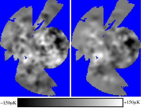
FIG. 1.: Visual comparison of the QMASK (left) and WMAP (right) maps, both Wiener filtered with the same weighting (determined by the QMASK noise covariance matrix). The slightly larger fluctuation level seen in the left image gives a visual indication of the effect of QMASK noise.

to perform end-to-end tests that are able to detect unforeseen problems as well. By far the most powerful test (in the statistical sense of being more likely to discover systematic errors) involves a direct comparison of the sky maps from experiments that overlap in both spatial and angular coverage, rather than merely a comparison of the measured angular power spectra. Some of the best testimony to the quality of CMB maps comes from the success of such map comparisons in the past — between FIRS and DMR [19], Tenerife and DMR [20], FIRAS and DMR [21], MSAM and SK (Saskatoon) [22], QMAP and SK [23], QMASK and DMR [24], PIQUE and SK [25], POLAR and DMR [26], DMR and WMAP [2], Maxima and WMAP [27], BOOMERanG and WMAP [28], Tenerife and WMAP [29], two years of Python data [30], four years of DMR data [31], three years of SK data [32], two flights of MSAM [33], and different channels of QMAP [7, 8, 9], BOOMERanG [11], MAXIMA [12], and WMAP [18]. It has now become possible to perform such tests with unprecedented sensitivity, using the spectacularly clean and well-tested WMAP data [2] as the answer sheet against which to compare other maps. So far, this has only been done carefully (beyond simple visual comparisons) for MAXIMA, with encouraging results [27]. This work showed that the WMAP-MAXIMA cross power spectrum was consistent with the power spectra measured from the two experiments separately.

The purpose of this letter is to carry out such a test for the QMASK data, which was the largest publicly available degree-scale CMB map prior to the WMAP release, and covers more than six times the area of the MAXIMA-I map. Not only was this map created using the above-mentioned Fourier and matrix techniques, but it combines measurements from both the ground-based SK experiment [5] and two balloon-based data sets from the QMAP experiment [7, 8, 9], therefore being potentially vulnerable to almost any systematic error one could imagine.

Although the two maps have different angular resolutions, their comparison is straightforward since the WMAP data is effectively noiseless (compared to the QMASK map) and can easily be smoothed to the QMASK angular resolution. Below we compare these two data sets using four different statistical tests, then present our conclusions in Section III.

II METHODS & RESULTS

A Data sets used in the analysis

The QMASK map was constructed from the combination of the SK and QMAP data sets [24]. It consists of 6590 pixels arranged on a simple square grid in gnomonic equal area projection, and its angular resolution corresponds to a Gaussian beam with FWHM $0.68^{\circ}$. These pixels are conveniently arranged in a 6590-dimensional vector ${\bf x}$ whose noise covariance matrix $\rm\bf N_{\rm QMASK}\equiv\langle{\bf x}{\bf x}^{t}\rangle$ is known and available online [24]. We compare it with both the WMAP Q-band map [2] and a foreground-cleaned CMB map made from a combination of the five WMAP CMB maps [34], hereafter TOH03. Before performing any analysis, the WMAP-Q and TOH03 maps were smoothed to have the same net beam function as QMASK, and data that do not overlap the QMASK observing region were discarded.

B Visual Comparison

We begin with a simple visual comparison. Comparing plots of the raw maps of QMASK (${\bf x}$) and WMAP (${\bf y}$) is not particularly useful, since QMASK is a noisy data set. Instead, we compare Wiener-filtered versions of both maps:

$${{\bf x}}^{w}=\rm\bf W{\bf x},\quad{{\bf y}}^{w}=\rm\bf W{\bf y},$$ (1)

where

$$\rm\bf W=\rm\bf S[\rm\bf S+\rm\bf N_{\rm QMASK}+\rm\bf N_{\rm WMAP}]^{-1},$$ (2)

and $\rm\bf S$ is the contribution to the map covariance matrix from CMB signal. The WMAP noise is so much smaller than that of QMASK that its exact value is irrelevant for our applications, so we make the approximation $\rm\bf N_{\rm WMAP}\approx 0$, i.e.,

$$\rm\bf W\approx\rm\bf S[\rm\bf S+\rm\bf N_{\rm QMASK}]^{-1}.$$ (3)

This linear filtering maximizes the signal-to-noise ratio in the QMASK map by effectively smoothing the map and downweighting noisy pixels and modes. Equation (1)  shows that to ensure a fair comparison, we Wiener-filter the WMAP map using the exact same $\rm\bf W$-matrix as for the QMASK map. The Wiener filtered QMASK map ${{\bf x}}^{w}$ (left) and WMAP TOH03 map ${{\bf y}}^{w}$ (right) are shown in Figure 1, and are seen to look encouragingly similar. Even the “anomalous” cold-spot around (RA,DEC)=($3^{h}20^{m}$, $84^{\circ}55^{{}^{\prime}}$) discussed in the QMASK analysis [24] (also seen by SK [35] but not by DMR [24]) is clearly visible in the WMAP data. The results are found to depend only weakly on the detailed choice of $\rm\bf S$. We wish to keep our map comparisons as theory-free as possible, and therefore choose $\rm\bf S$ corresponding to a simple scale-invariant spectrum with $\delta T_{\ell}=30\mu K$ here and below.

C Cross-correlation results

Next, we compare the QMASK and WMAP maps by cross-correlating them. The measured cross-correlation coefficient $\widehat{{\rm a}}$ and its variance $\Delta{\rm a}$ are given by [36]

$$\widehat{{\rm a}}={{\bf y}^{T}{\bf C}^{-1}{\bf x}\over{\bf y}^{T}{\bf C}^{-1}{\bf y}},$$ (4)

$$\Delta{\rm a}^{2}\equiv\langle\widehat{{\rm a}}^{2}\rangle-\langle\widehat{{\rm a}}\rangle^{2}=\left[{\bf y}^{T}{\bf C}^{-1}{\bf y}\right]^{-1},$$ (5)

where the covariance matrix ${\bf C}$ is defined as

$${\bf C}\equiv\rm\bf N+\rm\bf S=\rm\bf N_{\rm QMASK}+\rm\bf S.$$ (6)

As a first reality check, we cross-correlate the full QMASK data with the TOH03 map, obtaining $\widehat{{\rm a}}=0.921\pm 0.061$. This provides an encouraging validation of the QMASK observations, showing a detection of CMB signal at about the $15\sigma$ level. This also confirms and further strengthens the results of [24], who cross-correlated QMASK and DMR data [1, 31] and concluded that the CMB signal was consistent between the two data sets. It also provides a completely independent test of the accuracy with which the QMAP and SK experiments were calibrated, showing that they got things right to well within the quoted 10% calibration uncertainty [24].

Using only the sky area above $|b|>20^{\circ}$ (a Galactic cut), we detect the CMB signal at the $14.7\sigma$ level ($\widehat{{\rm a}}=0.938\pm 0.064$), and for a $|b|>30^{\circ}$ Galactic cut the detection is around the $9\sigma$ level ($\widehat{{\rm a}}=0.950\pm 0.110$). The similarity between the 20^∘ and 30^∘ cut results also confirms the conclusion of [37] that QMASK foregrounds are not dominant at high Galactic latitudes ($b>$20^∘).

D The $\chi^{2}$-test

A simple and robust way to test for discrepancies between the QMASK and WMAP maps is to calculate $\chi^{2}$ defined by

$$\chi^{2}\equiv{\bf z}^{T}\rm\bf N^{-1}{\bf z}\approx\widehat{{\rm a}}^{-2}{\bf z}^{T}\rm\bf N^{-1}_{\rm QMASK}{\bf z},$$ (7)

where ${\bf z}=\widehat{{\rm a}}{\bf x}-{\bf y}$ is the difference of the two maps after adjusting the QMASK calibration to the best-fit value found in the previous section. In the absence of systematic or calibration errors, the corresponding difference map should contain pure noise, so we should have $\langle{\bf z}\rangle$=0 and $\chi^{2}/N_{pix}\approx 1$, where $N_{pix}=6590$ is the number of pixels in the QMASK map vector ${\bf x}$. This is precisely what we find: we obtain $\chi^{2}/N_{pix}\approx 1.00$, i.e., the difference map ${\bf z}$ is consistent with pure noise. This means that the strong signal seen in Figure 1 is common to both maps and due to a true sky signal, with no evidence for significant systematic errors in QMASK.

E The Null-buster test

How statistically significant is our detection of signal in the maps? Consider the null hypothesis that a map ${\bf z}$ contains merely noise, i.e., $\langle{\bf z}{\bf z}^{T}\rangle=\rm\bf N$. Given the alternative hypothesis $\langle{\bf z}{\bf z}^{T}\rangle=\rm\bf N+\rm\bf S$, one can show that the most powerful “null-buster” test for ruling out the null hypothesis is using the statistic [38, 24]

$$\nu\equiv{{\bf z}^{T}\rm\bf N^{-1}\rm\bf S\rm\bf N^{-1}{\bf z}-\hbox{tr}\,\rm\bf N^{-1}\rm\bf S\over\left[2\,\hbox{tr}\,\left\{\rm\bf N^{-1}\rm\bf S\rm\bf N^{-1}\rm\bf S\right\}\right]^{1/2}},$$ (8)

which can be interpreted as the number of “sigmas” at which the null noise-only hypothesis is ruled out. Whenever we have reason to suspect systematic errors of a certain form are producing a signal $\propto\rm\bf S$, the null-buster test is more sensitive to these systematic errors than the

FIG. 2.: Null-buster comparison of QMASK (left) and WMAP-Q (right). This figure shows the number of standard deviations (“sigmas”) at which the difference map ${\bf z}={\bf x}-{\rm r}{\bf y}$ is inconsistent with pure noise.

$\chi^{2}$-test described in the previous subsection, which is a general-purpose tool.

The presence of foreground contamination (see [39] for a review) has been quantified independently for both the SK [36] and QMAP [37] experiments, by cross-correlating them with various foreground templates. The contamination level was found to be small enough to have negligible impact on the measured QMASK power spectrum [40], but as we will see below, it is nonetheless large enough to affect the more sensitive test we are performing here. The main QMASK foregrounds are synchrotron radiation, free-free emission and perhaps spinning dust emission, all of which become more important (relative to the CMB) at lower galactic latitudes and on larger angular scales (low $\l$). To focus on the CMB signal, Figure 2 therefore shows the nullbuster test results limited to $|b|>30^{\circ}$ and angular scales $\l\geq 30$. The latter is achieved by summing only over $\l=30,...,200$ when computing $\rm\bf S$ in equation (8)  (beam issues limit QMASK to $\l\mathrel{\hbox to0.0pt{\lower 3.0pt\hbox{$\mathchar 536\relax$}\hss}\raise 2.0pt\hbox{$\mathchar 316\relax$}}200$ [40]). This also corresponds to the angular range in which QMASK carries the bulk of its information, since limited sky coverage and angular resolution limit the information at $\ell\ll 30$ and $\l\gg 200$, respectively.

Figure 2 shows that whereas QMASK (left; $r=0$) and WMAP-Q (right; $r=\infty$) detect sky signal at the level of about $30\sigma$ and $2300\sigma$, respectively, the difference map (corresponding to $r$=1) is consistent with pure noise, and the null hypothesis of no systematic errors fails at less than $2\sigma$ level. The fact that the curve has such a narrow minimum at $r\sim 1$ also provides a strong confirmation that the relative calibration of QMASK and WMAP is good.

We used the WMAP-Q map for this test because it is closest in frequency to that of the QMASK map, which is constructed from a combination of Ka- and Q-band data. We also repeated the nullbuster test using the foreground-cleaned TOH03 WMAP map, finding marginally worse agreement as expected, since this compares a map that includes foregrounds with an essentially foreground-free map. As expected, the agreement between the two maps also deteriorated when including data at lower Galactic latitudes, where foregrounds become more important.

III CONCLUSIONS

In summary, a powerful set of FFT- and matrix-based tools have been developed in recent years for producing quality CMB maps from time-ordered observations. Although these tools are mathematically elegant, there have been few precision tests of how well they work in practice when faced with real-world systematic errors from suborbital experiments. We have performed a precision test of precisely this, comparing the QMASK map with the “answer sheet” provided by WMAP. The results are very encouraging, showing excellent agreement and no statistically significant evidence of residual systematic errors. This suggests that although space-based observations will obviously be required for many tasks, e.g., all-sky mapping of CMB polarization, suborbital experiments have the potential to continue playing a key role in the precision cosmology era.

The authors wish to thank David Spergel for useful comments and the WMAP team for producing such a superb data set and making it public via the Legacy Archive for Microwave Background Data Analysis (LAMBDA), supported by the NASA Office of Space Science. This work was supported by NASA grant NAG5-11099, NSF grants AST-0134999 and AST9732960, and fellowships from the David and Lucile Packard Foundation and the Research Corporation.

REFERENCES

- [1] G. F. Smoot et al., ApJ 396, L1 (1992).
- [2] C. L. Bennett et al., astro-ph/0302207 (2003).
- [3] M. Tegmark, ApJL 480, L87 (1997).
- [4] M. Tegmark, PRD 56, 4514 (1997).
- [5] C. B. Netterfield, M. J. Devlin, N. Jarosik, L. A. Page, and E. J. Wollack, ApJ 474, 47 (1997).
- [6] M. Tegmark, A. de Oliveira-Costa, J. Staren et al., ApJ 541, 535-541 (1999).
- [7] M. Devlin, A. de Oliveira-Costa, T. Herbig, A. D. Miller, C. B. Netterfield, L. A. Page, and M. Tegmark, ApJL 509, L77 (1998).
- [8] T. Herbig, A. de Oliveira-Costa, M. Devlin, A. D. Miller, C. B. Netterfield, L. A. Page, and M. Tegmark et al., ApJL 509, L73 (1998).
- [9] A. de Oliveira-Costa, M. Devlin, T. Herbig, A. D. Miller, C. B. Netterfield, L. A. Page, and M. Tegmark, ApJL 509, L77 (1998).
- [10] J. Borrill, astro-ph/9911389 (1999).
- [11] P. de Bernardis et al., Nature 404, 955 (2000).
- [12] S. Hanany et al., ApJL 545, L5 (2000).
- [13] R. Stompor et al., PRD 65, 022003 (2002).
- [14] B. Wandelt, E. Hivon, and K. M. Gorski, PRD 64, 3003 (2001).
- [15] N. W. Halverson et al., ApJ 568, 38 (2002).
- [16] E. Hivon, K. M. Gorski, C. B. Netterfield, B. Crill, S. Prunet, and F. Hansenrode, ApJ 567, 2 (2002).
- [17] S. T. Myers et al., ApJ 591, 575 (2003).
- [18] G. Hinshaw et al., ApJS 148, 63 (2003).
- [19] K. Ganga, E. Cheng, S. Meyer, and L. Page, ApJL 410, L57 (1993).
- [20] C. H. Lineweaver et al., ApJ 448, 482 (1995).
- [21] D. Fixsen, G. Hinshaw, C. L. Bennett, and J. C. Mather, ApJ 486, 623 (1997).
- [22] L. Knox, J. R. Bond, A. H. Jaffe, M. Segal, and D. Charbonneau, PRD 58, 083004 (1998).
- [23] A. de Oliveira-Costa et al., ApJ. 509, L77 (1998).
- [24] Y. Xu, M. Tegmark, A. de Oliveira-Costa, M. Devlin, T. Herbig, A. D. Miller, C. B. Netterfield, and L. A. Page, PRD 63, 103002 (2001).
- [25] A. de Oliveira-Costa et al., PRD 67, 023003 (2003).
- [26] A. de Oliveira-Costa et al., PRD 68, 3003 (2003).
- [27] M. E. Abroe et al., ApJ 605, 607 (2004).
- [28] P. de Bernardis et al., IAU Symposium 216: Maps of the Cosmos (2003).
- [29] A. de Oliveira-Costa et al., ApJ 606, L89 (2004).
- [30] J. E. Ruhl et al., ApJL 453, L1 (1995).
- [31] C. L. Bennett et al., ApJ 464, L1 (1996).
- [32] M. Tegmark et al., ApJL 474, L77 (1996a).
- [33] C. A. Inman et al., ApJL 478, L1 (1997).
- [34] M. Tegmark, A. de Oliveira-Costa, and A. Hamilton, PRD 68, 123523 ( 2003).
- [35] E. J. Wollack et al., ApJ 419, L49 (1993).
- [36] A. de Oliveira-Costa, A. Kogut, M. J. Devlin, C. B. Netterfield, L. A. Page, E. J. Wollack, ApJ 482, L17 (1997).
- [37] A. de Oliveira-Costa et al., ApJL 542, L5 ( 2000).
- [38] M. Tegmark, ApJ 519, 513 (1999).
- [39] M. Tegmark, D. J. Eisenstein, W. Hu, and A. de Oliveira-Costa, ApJ 530, 133 (2000).
- [40] X. Yongzhong, M. Tegmark, and A. de Oliveira-Costa, PRD 65, 083002 (2002).