Automated Nonlinear Stellar Pulsation Calculations:  Applications to RR Lyrae stars

We describe a methodology that allows us to follow the pulsational behavior of an RR Lyrae model consistently and automatically along its evolutionary track throughout the whole instability strip. It is based on the powerful amplitude equation formalism, and resorts to a judicious combination of numerical hydrodynamical simulations, the analytical signal time-series analysis, and amplitude equations.

A large-scale survey of the nonlinear pulsations in RR Lyr instability strip is then presented, and the mode selection mechanism is delineated throughout the relevant regions of parameter space. We obtain and examine two regions with hysteresis, where the pulsational state depends on the direction of the evolutionary tracks, namely a region with either fundamental (RRab) or first overtone (RRc) pulsations and a region with either fundamental (RRab) or double-mode (RRd) pulsations.

The regions where stable double-mode (DM, or RRd) pulsations occur are very narrow and hard to find in astrophysical parameter ($L$, $M$, ${T_{\rm ef\!f}}$, $X$, $Z$) space with hydrodynamic simulations, but our systematic and efficient methodology allows us to investigate them with unprecedented detail.

It is shown that by simultaneously considering the effects of mode selection and of horizontal branch evolution we can naturally solve one of the extant puzzles involving the topologies of the theoretical and observed instability strips, namely the slope of the fundamental blue edge.

The importance of the interplay between mode selection and stellar evolutionary effects is also demonstrated for the properties of double-mode RR Lyr. Finally, the Petersen diagram of double-mode RR Lyr models is discussed for the first time.

1 Introduction

The evolutionary tracks of the classical variable stars carry them once or more through the instability strip (IS) where they can undergo pulsations of various types, such as single-mode pulsations in the fundamental (F), in the first overtone (O1), in the second overtone (O2), or double-mode (DM) pulsations. The latter are beat pulsations that occur either in the F and O1 modes or in the O1 and O2 modes. A beautiful observational summary for the Cepheids is provided by the microlensing projects, e.g.  Beaulieu et al. (beau97 (1997)) or Udalski et al. (Udalski (1999)). Thus low luminosity Cepheids are seen to undergo DM pulsations, whereas this phenomenon does not occur for the high luminosity ones. In the intermediate luminosity range single-mode F and O1 Cepheids seem to overlap, and in the high luminosity regime there are only F Cepheids. For RR Lyrae the picture is similar, except that there is another type of modulated pulsation (the Blazhko effect) that has not received a satisfactory explanation to date.

Theory of course aims to understand the observed modal behavior and to provide a global picture thereof. In this paper we merge several techniques that have been used separately and combine them into an efficient methodology that allows one to follow the pulsational behavior of a star along its full evolutionary track, from the moment it enters the IS till it leaves it.

These tools are then applied to open questions and relatively unexplored topics concerning the radial pulsations of RR Lyr stars. Since the first claim of a successful modelling of double-mode pulsation with a turbulent convective code (Feuchtinger feuchtinger1 (1998), Kolláth et al. kollath3 (1998)), no systematic exploration of the RRd models has been published except for some limited studies (Szabó et al. rszabo (2000)). Here we attempt to remedy this situation. In the process of studying double-mode RR Lyr we have also uncovered a hidden relation between evolution and pulsation.

Another question concerns the discrepant topologies of the theoretical and the empirical RR Lyr ISs (Jurcsik jurcsik97 (1997)). A series of papers (Kovács & Jurcsik kj1 (1996), kj2 (1997); Jurcsik jurcsik (1998)) establishes empirical relations between RRab light-curve parameters and absolute magnitudes, colors and metallicities. These quantities are further transformed to the ${T_{\rm ef\!f}}-L$ plane via  Kurucz’s static model atmospheres. (We mention in passing that such empirical relations do not yet exist for the overtone RRc stars.) For the distribution of RRab stars the empirical ${\rm Log}\thinspace{T_{\rm ef\!f}}-{\rm Log}\thinspace L$ diagram shows a well-defined and straight edge. However, attempts at reproducing the empirical RR Lyr F and O1 blue edges have failed: neither radiative nor convective models could explain the shallow slope of the blue edges of the F and O1 instability regions (Kolláth et al. kbf (2000), KBF). Despite the investigation of a large number of physical effects that might change the slopes, such as rotation, exotic chemical abundances, radiative transport, KBF could not offer an explanation for the shallow slope of the empirical F blue edge. Throughout this paper we shall refer to this problem as the fundamental blue edge problem. Using our new methodology, we will demonstrate that the solution to the problem lies in the simultaneous taking into account both mode selection and stellar evolution.

Because of an ambiguous use of the notion of DM or beat pulsations in the literature, at the risk of being pedantic, we need to address this issue briefly. We talk about DM pulsations of a given stellar model, with fixed $L$, $M$ and $T_{\rm ef\!f}$ when (a) the Fourier spectrum exhibits two dominant frequency peaks and those corresponding to all the linear combinations of these two, and (b) the amplitudes of all the peaks are constant. When the pulsations of a stellar model display this type of spectrum, but the amplitudes vary slowly compared to the period (but still fast compared to evolution), then such a model is in the process of switching modes – it may or may not ultimately end up as a true DM pulsator. In fact, it may just be switching from one single mode state to another, say F to O1, if it is in a so-called either F or O1 region. But these different scenarios correspond to stellar models with different physical parameters. For a real star, $L$ and $T_{\rm ef\!f}$ are not constant, but change as the star moves along its evolutionary track. How this evolution affects mode switching has recently been discussed by Buchler & Kolláth (bk02 (2002), hereafter BK2002). From an observational point of view it may not be possible to discriminate between stars that are switching from RRab to RRc (or RRc to RRab) and actual RRd stars, but at least, in principle, they should be distinguished.

The layout of the paper is the following: the methodology is presented in Sec. 2., and it is applied in a large-scale nonlinear survey of radial RR Lyr pulsation in Sec. 3. In Sec. 4. mode selection characteristics are discussed including the systematic mapping of the DM pulsation region of RR Lyr stars. The F blue edge problem is revisited in Sec. 5., testing the combined effects of the mode selection and horizontal-branch (HB) stellar evolution on the structure of the RR Lyr IS. Three different sets of HB evolutionary tracks are considered to account for realistic evolutionary changes of stellar parameters. In Sec. 6. an hitherto unknown connection is uncovered between double-mode pulsation and evolution, as well as the Petersen diagram of nonlinear RRd models is discussed. Finally, we conclude in Sec. 7.

2 The Methodology

2.1 Timescales and Amplitude Equations (AEs)

Stellar pulsations are characterized by three timescales, generally well separated in size. The shortest is the dynamic time, $\tau_{dyn}$, which corresponds to the period or cycling time. Next comes the transient time scale, $\tau_{trans}$, on which the amplitudes change during mode switching, e.g.  from F to O1 pulsation; this can be, but need not be, the thermal timescale given by the inverse growth-rate (BK2002). The longest timescale is the stellar evolution time, $\tau_{evol}$, i.e.  the timescale corresponding to nuclear burning in the core.

The AE formalism (Buchler & Goupil BuchlerG (1984)) was developed to enable us to study the pulsation problem on the longer timescales, by averaging out the dynamic timescale, i.e.  the rapidly varying phases ($\exp i\omega_{k}t)$. The AEs are differential equations which no longer contain the frequencies, and which govern the behavior of the amplitudes of the most relevant modes on both the transient and on the evolutionary timescales.

In RR Lyr the F and the O1 are the only relevant modes for the pulsation problem. Furthermore there are no resonances between these modes, nor with their overtones, and the apposite AEs are (Buchler & Goupil BuchlerG (1984)):

$$\dot{A}_{\rm 0} = \big{(}\kappa_{0}(\xi)+q_{00}(\xi)A_{\rm 0}^{2}+q_{01}(\xi)A_{\rm 1}^{2}$$ (1)

$$\quad\quad\quad+s_{0}(\xi)A_{\rm 0}^{2}A_{\rm 1}^{2}+r_{0}(\xi)A_{\rm 0}^{4}\big{)}{\thinspace}\ A_{\rm 0}$$

$$\dot{A}_{\rm 1} = \big{(}\kappa_{1}(\xi)+q_{10}(\xi)A_{\rm 0}^{2}+q_{11}(\xi)A_{\rm 1}^{2}$$ (2)

$$\quad\quad\quad+s_{1}(\xi)A_{\rm 0}^{2}A_{\rm 1}^{2}+r_{1}(\xi)A_{\rm 1}^{4}\big{)}{\thinspace}\ A_{\rm 1}$$

The subscripts 0 and 1 refer to the F and the O1 modes. The quantities $\kappa_{k}$ represent the linear growth-rates of the two modes, the $q$s the cubic, and the $s$’s and $r$’s the quintic coupling coefficients for a given model. In Kolláth et al. (kollath2 (2002), KBSC) it has been demonstrated that we can drop the $r$ terms without prejudice. All these quantities are functions of the model parameters $\xi=(L,{T_{\rm ef\!f}},M,{\rm composition})$, where $T_{\rm ef\!f}$ represents the effective temperature of the equilibrium model.

As far as pulsation modelling is concerned the evolutionary tracks for a given mass $M$, provide us with a luminosity $L(t)$, and effective temperature $T_{\rm ef\!f}(t)$, i.e. they specify the time-dependence of the $\xi$. The stellar envelopes have a uniform composition having recently undergone a fully convective stage. We recall that for a given composition, specified by $X$ and $Z$, for example, these three quantities $M$, $L$ and $T_{\rm ef\!f}$ uniquely specify the stellar envelope, i.e. without a need to know the properties of the stellar interior. (One could equivalently, but much less conveniently characterize the stellar envelope instead by the luminosity, temperature and pressure at the core radius, for example). Controversies associated with core convection and overshooting thus need not concern us here because pulsation is limited to the part of the star (the envelope) that is located above the burning shells (i.e. $T<$ a few million K).

Figure 1: Flow vector fields for two RR Lyr models on the ($A_{0},A_{1}$) phase-space (the dots denote the bases of the normalized vectors). The large dots represent the hydrodynamical transients for several different initializations (kicks). The dots represent equal time-intervals, so that the spacing of the dots indicates of the speed. a.) F/O1 model ($M=0.71\thinspace{\rm M_{\sun}}$, $L=50\thinspace{\rm L_{\sun}}$, $T_{\rm ef\!f}=6700{{\thinspace}{\rm K}}$, $Z=0.0001$). The stable F and O1 limit cycles denoted by filled hexagons are located at ($0.0483\thinspace;0.0000$) and ($0.0000\thinspace;0.0285$), respectively, and the presence of an unstable DM (open hexagon) can be seen on the arc at ($0.0282\thinspace;0.0188$). b.) F/DM model ($M=0.77\thinspace{\rm M_{\sun}}$, $L=50\thinspace{\rm L_{\sun}}$, $T_{\rm ef\!f}=6510{{\thinspace}{\rm K}}$, $Z=0.001$). The stable fundamental and double-mode fixed points are located at ($0.0515\thinspace;0.0000$) and ($0.0116\thinspace;0.0274$), respectively. The unstable O1 and DM fixed points can be found at ($0.0000\thinspace;0.0286$) and ($0.0205\thinspace;0.0242$).

It is useful to introduce the quasi-static approximation (QSA) which consists of disregarding the time-dependence of the $\xi$. The stellar model is thus considered frozen at a point along its evolutionary track. The QSA serves two purposes. First, the AEs with the QSA, i.e. Eqs. 1– 2. with fixed constant coefficients, describe the temporal (transient) behavior of the modal amplitudes of a stellar model with fixed $M$, $L$ and $T_{\rm ef\!f}$. The QSA thus provides an excellent description of the transient pulsational behavior of a given stellar model from some initial conditions toward its asymptotic limit cycle or DM pulsation, as the case may be. Conversely, the hydrodynamic evolution of such a model can be employed to extract the coefficients of the AEs for given $M$, $L$ and $T_{\rm ef\!f}$.

Second, away from the bifurcation points, $\tau_{trans}\ll\tau_{evol}$, and the stellar model should be in (one of) its asymptotic pulsational states. Instead of having to integrate Eqs. 1– 2. one then only needs to calculate their fixed points, $\dot{A}_{k}=0$, which correspond either to limit cycles or to steady double-mode pulsations. When more than one asymptotic pulsational state is possible the star naturally stays in the one that is closest to the one it had at an earlier instant. Hysteresis is possible when evolutionary tracks run in opposite directions at different stages of the evolution.

In summary then, if we can compute the $\kappa_{k}$ and the coupling coefficients as a function of $L$ and $T_{\rm ef\!f}$ from pulsation theory on the one hand, and the time-dependence of the latter from the evolutionary tracks, on the other, we can then integrate Eqs. 1– 2. to obtain $A_{k}(t)$ along the whole track, including mode switchings, also called bifurcations (BK2002).

We note in passing that the more complicated situation $\tau_{trans}\sim\tau_{evol}$ that always occurs near changes of stability (bifurcation points) has recently been examined by BK2002.

2.2 The Nonlinear Coupling Coefficients

One finds that the growth-rates and the coefficients vary smoothly with $T_{\rm ef\!f}$, $L$, and $M$. Consequently it is sufficient to compute these coefficients for only a few stellar models with fixed $T_{\rm ef\!f}$ and $L$ inside the IS, and the intermediate values along the track can then be obtained by interpolation. In sharp contrast, the amplitudes, solutions of the AEs, and the pulsational states can vary very rapidly with $T_{\rm ef\!f}$ and $L$.

The computation of the coupling coefficients of a given model, with a specified $T_{\rm ef\!f}$, $L$ and composition proceeds in a few steps (Kolláth & Buchler kb01 (2001)).

2.2.1 The hydrodynamical calculations

The star can reach more than one type of full amplitude pulsation depending on the initial conditions (several basins of attraction). The most familiar case is the coexistence of either F or O1 limit cycles, but they can also be steady double-mode (DM) pulsations. In that case it is important to choose initial perturbations so that the transient tracks sample enough of the amplitude-amplitude plane. Thus, for several suitably chosen initial perturbations of the (pulsationally unstable) equilibrium model we follow its transient pulsational behavior with numerical hydrodynamics until the achievement of steady, or almost steady full amplitude pulsations.

In this paper we investigate pulsation from dynamical point of view, and we do not consider light-curves and velocity curves. The interested reader is referred to Kolláth & Buchler (kb01 (2001)). We note that light and velocity curves are in good agreement with the observations and an accurate radiative transfer rather than radiation diffusion as we use has little effect on the bolometric light curves. More detailed computations from the point of view of color dependence of LCs have been made by Dorfi & Feuchtinger (df (2000)).

2.2.2 The analytical signal method

The output from each of the hydrodynamical calculations, for example the stellar radius $R_{*}(t)$, is subjected to the analytical signal (time-frequency) analysis (Gábor gabor (1946)). This provides the time-dependence of the amplitudes $A_{k}(t)$ (KBSC). Astrophysicists are generally familiar with this procedure because of the Kramers–Kronig dispersion relations (Jackson jackson (1975)). One considers the signal $s(t)$ to represent the real part of an assumed complex analytical function $a(t)$. The imaginary part $\tilde{s}(t)$ of $a(t)$ can then be obtained via  Cauchy’s formula, which is converted to a Hilbert transform, and finally to a Fourier transform and a subsequent one-sided reverse Fourier transform. The advantage of the latter formulation is that both are extremely fast to perform (cf. e.g. Cohen cohen (1994)).

$$a(t) \negthinspace\negthinspace\negthinspace=\negthinspace\negthinspace\negthinspace s(t)+i\tilde{s}(t)=s(t)+\frac{i}{\pi}{\thinspace}PV{\thinspace}\int_{-\infty}^{\infty}dt^{\prime}\frac{s(t^{\prime})}{t-t^{\prime}}$$ (3)

$$\negthinspace\negthinspace\negthinspace=\negthinspace\negthinspace\negthinspace \frac{1}{\pi}\int^{\infty}_{0}d\omega e^{i\omega t}\int_{-\infty}^{\infty}dt^{\prime}s(t^{\prime})e^{-i\omega t^{\prime}}$$

$$\negthinspace\negthinspace\negthinspace\equiv\negthinspace\negthinspace\negthinspace A(t){\thinspace}{\thinspace}e^{i\varphi(t)}$$

With this procedure it is therefore very easy to determine unambiguously the instantaneous phase $\varphi(t)$ and amplitude $A(t)$ of a signal.

The method is extended to multi-component signals with the help of filters that restrict the power to the desired frequency components. It is convenient to make this filtering in Fourier space where it involves just a product, and to combine it with the definition of the analytical signal

$$Z_{k}(t) \negthinspace\negthinspace\negthinspace=\negthinspace\negthinspace\negthinspace A_{k}(t)e^{i\varphi_{k}(t)}$$ (4)

$$\negthinspace\negthinspace\negthinspace=\negthinspace\negthinspace\negthinspace \frac{1}{\pi}\int^{\infty}_{0}\negthinspace\negthinspace\negthinspace d\omega H(\omega-\omega_{k})e^{i\omega t}\negthinspace\int_{-\infty}^{\infty}\negthinspace\negthinspace\negthinspace dt^{\prime}s(t^{\prime})e^{-i\omega t^{\prime}},$$

where $H(\omega-\omega_{k})$ is the filtering window, centered on the desired $\omega_{k}$. Generally, a Gaussian window with a half width of 0.2 c/d provides satisfactory results.

Figure 1a. illustrates the amplitude evolution of an RR Lyr model that has both an F and an O1 limit cycle. The origin is unstable (equilibrium model), and depending on the initial kick the model goes to one or the other limit cycle. In addition to these limit cycles, there exists an unstable DM that is clearly visible along the arc. An example of another, more complicated phase-portrait involving two DMs can be found in Fig. 1b. There are two stable fixed points here: a DM and an F. This stable DM pulsation exhibits a dominant overtone pulsation amplitude.

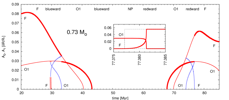
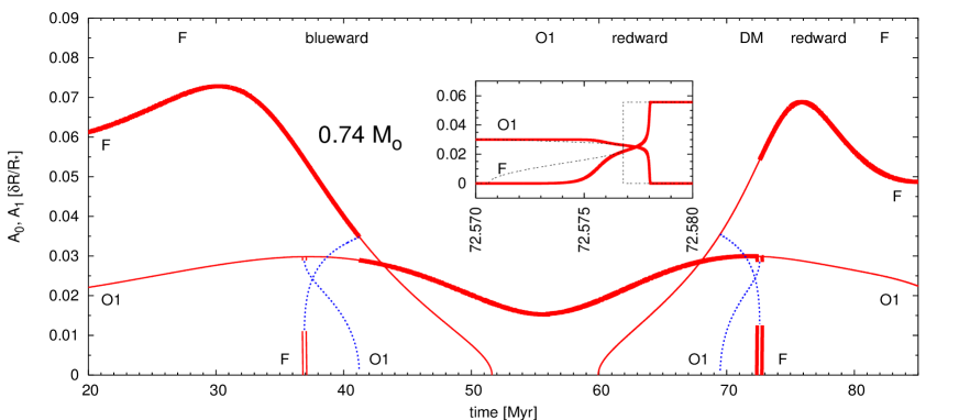
Figure 2: Evolution of the amplitudes and component amplitudes of two RR Lyr models (with $Z=0.0001$) throughout the IS; upper panel: $M=0.73\thinspace{\rm M_{\sun}}$ lower panel: $M=0.74\thinspace{\rm M_{\sun}}$. The thick lines represent the pulsational modal amplitudes that actually achieved attained along the track, the thin lines potential pulsation states, the dotted lines the amplitudes of unstable double-mode pulsation. The stable DM amplitudes are represented by double lines. DM pulsation occurs during the redward evolution of the higher mass model. The attained pulsation mode and the direction of the evolution are indicated on top; NP denotes the non-pulsating interval during which the star leaves the instability strip. The insets represent blowups of the amplitudes during the redward mode switching phases that last a few thousand years. The broken lines in the insets show the QSA amplitudes, i.e. the amplitudes that would occur if the pulsation could adjust instantaneously to the asymptotic limit cycle of DM pulsation of the model with the current $M$, $L$ and $T_{\rm ef\!f}$. Compare with Fig. 5.

2.2.3 The linear least-squares fit

Once the temporal behavior of the amplitudes has been obtained we can determine the coupling coefficients and the linear growth-rates with a linear least-squares fit from Eqs. 1– 2. in which $\xi$ is fixed to the values of $M$, $L$ and $T_{\rm ef\!f}$ that have been used in the hydrodynamical computations.

The fit is linear because the analytical signal analysis yields amplitudes that are smooth enough to compute time-derivatives, and it is not necessary to fit the transients to integral curves of Eqs. 1– 2. as with the older technique (Buchler & Kovács bk87 (1987); Kovács & Buchler bk93 (1993); Kovács et al. kbd (1987)).

2.2.4 The evolution of the pulsations

The previous procedure can be repeated for a sequence of models along the evolutionary track and the behavior of the growth-rates and coupling coefficients as a function of $T_{\rm ef\!f}$ and $L$ can then be obtained by interpolation. The solution of Eqs. 1– 2. allows us to follow the pulsational behavior of our model along its evolutionary track once we know the temporal behavior of the $\kappa$s and of the coefficients because of slow stellar evolution. For that transformation we need $T_{\rm ef\!f}(t)$ and $L(t)$ which are obtained from published stellar evolution calculations, e.g.  Schaller et al. (ssmm (1992)); Alibert et al. (alibert (1999)) for Cepheids, Dorman (dorman (1992)); Demarque et al. (demarque (2000)); Girardi et al. (girardi (2000)) for RR Lyr.

In Fig. 2. we present the evolution of the pulsation amplitudes of two RR Lyr models along their Demarque evolution tracks through the IS which are shown in Fig. 5. The $M=0.73\thinspace{\rm M_{\sun}}$ model starts up with F mode pulsation. Then, while evolving blueward, it changes to O1, and it finally leaves the IS temporarily. Next, it repeats these steps in reverse order while evolving redward. The higher mass model also experiences DM pulsation for a short period during its redward evolution, entering the F/DM hysteresis region (Sec. 3.2). We note that we have not made the QSA for the amplitudes and that we have considered the evolution induced delay in the switching (BK2002).

The insets of Fig. 2. enlarge the interval over which the righthand switchings take place. A scenario similar to the top inset, but with O1 and F interchanged takes place near 33 Myr for the $0.73\thinspace{\rm M_{\sun}}$ model, and near 41 Myr for the $0.74\thinspace{\rm M_{\sun}}$ model. For all of these switchings, which we termed hard in BK2002, the timescale is of the order of a few thousand years, much shorter than the evolution timescale, and somewhat longer than the thermal timescale. The broken lines in the insets present the QSA amplitudes, i.e.  the amplitudes that would obtain if the switch was instantaneous.

In the top inset the switch occurs from a stable O1 mode limit cycle to a stable F mode limit cycle. The transition is not sharp and there is a delay, both caused by evolution as explained in BK2002.

The situation in the bottom inset is more complicated. Here the switch occurs first from an O1 limit cycle to a DM state, then from the DM to the F limit cycle. Again, the two transitions are not sharp, but washed out by an evolution induced delay in the switching. The DM pulsation is in principle already possible at $\sim$72.5705 Myr, but because of evolution it gets delayed $\sim$4000 yrs. Subsequently, the F pulsation could start at $\sim$72.577, but gets delayed some 1000 years.

Observationally it would be very hard to distinguish between the switching from RRab to RRc (or vice-versa, as displayed in the inset in the top figure) on the one hand, and true RRd behavior, as seen in the bottom inset, on the other hand, although from a theoretical point of view they are very different.

Figure 2. clearly demonstrates that the time spent in the mode switching phases is very short compared to the RRab and RRc phases.

2.2.5 Resonances

It is well established that as the structure of the stellar envelope changes along the evolutionary track, resonances can occur between the excited mode and one or more overtones. The presence of resonances has a strong effect on the Fourier decomposition parameters of the light-curves and radial velocity curves (e.g.  Buchler Mito (1993)). In this paper we ignore the effects of resonances which is a valid assumption for RR Lyr stars, but would not be for Cepheids.

In summary, our new methodology makes it possible to follow in an automated fashion the full amplitude pulsational behavior along the tracks that stellar evolution computations provide.

3 Nonlinear RR Lyrae Models

3.1 Turbulent convective models

In order to explore the mode selection characteristics in numerical RR Lyr models, we have used the Florida-Budapest TC-codes (e.g.  Yecko et al. ykb (1998), KBSC), which are 1D, linear and nonlinear hydrocodes that include turbulent convection and are tailored to radial stellar pulsations.

The hydrogen content of the models is set to be $X=0.75$. The turbulent convection parameters are chosen as in KBSC (Table 1.) to ensure observed amplitudes. Model sequences for each combination of triplets ($L$, $M$, $Z$) from

• $M=0.50,0.55,0.60,0.65,0.71,0.77,0.82,(0.85),0.87{\rm M_{\sun}}$

• $L=40,\ 50,\ 60,\ 70\ {\rm L_{\sun}}$

• $Z=10^{-4},\ 10^{-3},\ 4\cdot 10^{-3}$

have been computed, in which only $T_{\rm ef\!f}$ is varied. No evolutionary constraints were applied in the parameter selection at this point. Applying the methodology described in Sec. 2. has allowed the interpolation of the limits of different pulsational states to an internal accuracy of $2-3{{\thinspace}{\rm K}}$ within a sequence, requiring the computation of only 8 to 10 models in a given sequence.

We have generated a large grid of models which contains mode selection information throughout the relevant regions of the parameter space. We note here again, that at this point we do not care about the existence of the objects represented by these models, as the whole model set is used only to point out mode selection characteristics (Sec. 4.). The existence will be ensured in Secs. 5-6., where evolutionary tracks are applied to select the astronomically relevant models among the complete set of computed models. This way, the presented results concerning the fundamental blue edge and the double-mode RR Lyrae stars are based on pulsational models that were naturally selected by evolutionary calculation constraints.

The following combinations of one or two stable fixed points are encountered in our models:

• fundamental mode (F)

• first overtone (O1)

• either first overtone or fundamental mode (F/O1)

• double-mode (DM)

• either fundamental or double-mode (F/DM)

Because the DM and F/DM regions are very narrow, they are difficult to find with hydrodynamical modelling, although Feuchtinger (feuchtinger1 (1998)) had the good fortune to actually encounter one! However, interpolation on our grid easily reveals their presence. Once their existence and their astrophysical parameters are known, it is not difficult to confirm the presence of DM pulsation through the computation of further models. We conclude that amplitude equation fitting is a robust and effective method in this sense.

We now turn to a discussion of the shortcomings and uncertainties in our model computations. The selection of turbulent convective parameters is not unique. We have found that the amplitude and the IS width requirements cannot be fulfilled at the same time for a given set of $\alpha$ parameters. We have therefore fixed turbulent parameters to give the correct observed amplitudes (magnitudes) as in KBSC (Table 1.), but that extended the location of the F linear red edge to very low temperatures, giving an excessive width to the F IS. On the other hand, it caused but a small excursion in all the other edges. If we were to apply a different set of $\alpha$s, a fine-tuning of the TC parameters would be necessary, and that would bring about small temperature shifts of $10-50{{\thinspace}{\rm K}}$. But these shifts would affect the mode selection regions as a whole, not changing the location of the edges with respect to each other (except F red edge). Therefore we think that, aside from small shifts in temperature our overall picture is correct, and we attained a good relative accuracy in determining mode selection.

3.2 Mode selection hysteresis

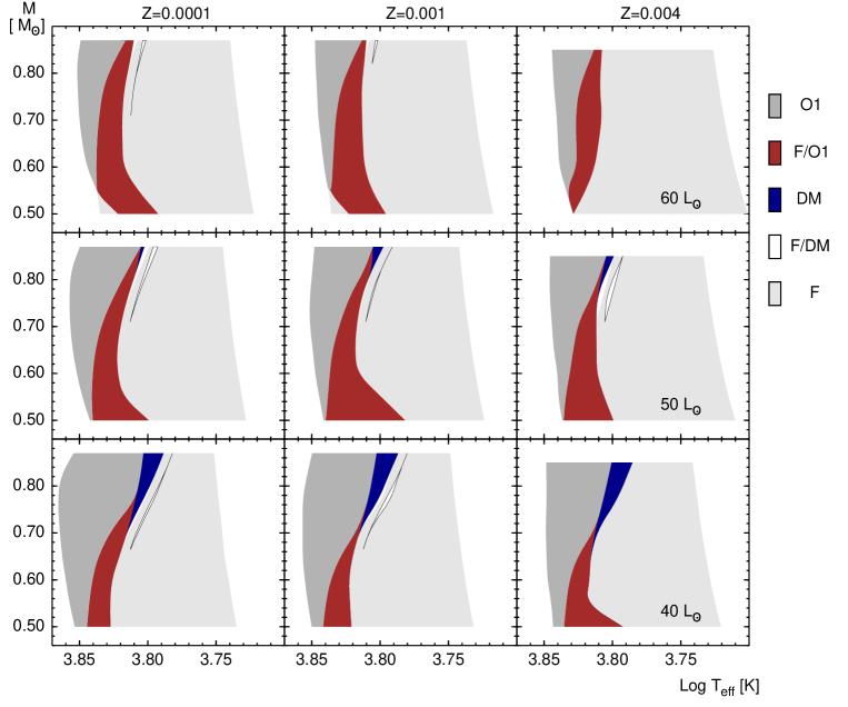
Figure 3:  Overview of the pulsation modes for RR Lyr stars as a function of stellar mass. Rows have fixed luminosity, columns contain fixed metallicity. Note that the models displayed in this figure were computed with arbitrary selections of mass, luminosity, temperature and metallicity to fully explore the mode selection characteristics. See text for details. The legend is the following: F: fundamental mode F/DM: either fundamental or double-mode DM: double-mode F/O1: either fundamental or first overtone (F/O1) O1: first overtone mode. Note that for the sake of clarity the F/DM region has been plotted shifted by 100 ${{\thinspace}{\rm K}}$ to the right in the Figures.

It is well known from the early suggestion of van Albada & Baker (albada (1973)) that in the case of classical pulsators there exists a region in the HR diagram in which either F or O1 pulsations are possible. Rather than follow the pulsation jargon of calling it the ’either-or-region’, we refer to it as a F/O1 region, especially since we will also encounter other types of hysteresis. Hysteresis here means that the pulsation state depends on the direction of evolution. For example, if the star evolves from low temperatures to high temperatures (blueward) in this region, it exhibits F mode pulsation (RRab in our case), while evolving in the opposite direction results in an O1 pulsator (RRc) with the same stellar parameters. This is the classical F/O1 region. Recent observational facts (Castellani et al. castellani (2003)), the amplitude equation formalism (Buchler & Kovács bk (1986)) as well as state-of-the-art numerical hydrodynamical calculations (KBSC) all concur that this behavior indeed exists.

It is interesting to note that we have encountered an additional hysteresis in the course of the present survey, namely an F/DM region where either F or DM pulsations are possible.

The width of the F/O1 region can be several hundred  ${\rm K}$, depending on the mass, luminosity, and metallicity. As stars with different parameters pass through this region, mode selection can significantly bend the average slope of the observed F blue edge. Therefore this effect supplemented by reliable evolutionary data has the potential of reproducing the slope of the RR Lyr F blue edge. One of the main motivations of this paper (Sec. 5) has been to investigate this scenario as a possible resolution of the puzzle that was discussed in KBF.

4 Mode selection maps

The computed mode selection maps are exhibited in Fig. 3., presented in the form of a $M$ – $T_{\rm ef\!f}$ plot. For the first time, double-mode regions are also included. We emphasize that the models of Fig. 3. were computed with arbitrary selections of mass, luminosity, temperature and metallicity, as was described in Sec. 3.1. Although some configurations of $M$, $L$, and $T_{\rm ef\!f}$ may well not actually exist in Nature, this method allows us to explore the mode selection characteristics throughout the whole parameters space. In addition, by reducing the parameter space (e.g. by applying evolutionary constraints) in order to minimize the time-consuming model computations, we could easily miss important features of the mode selection phenomenon. These models are later subject to merge with evolutionary tracks to end up with models of existing objects (Secs. 5-6.) in a self-consistent way. We now discuss the most important mode selection features:

– The topology of the IS is very similar but not identical for different metallicity values. Clear differences also exist in different luminosity panels and for different masses. It is in good agreement with the results of Bono & Stellingwerf (bono94 (1994)), namely with a redder F blue edge at lower luminosity levels. In terms of metallicity the difference manifests itself in the form of slight shifts in temperature, but typically less than $100{{\thinspace}{\rm K}}$. We caution though, that these small changes cannot be neglected when we derive the slope of the IS edges, as will be pointed out in Sec. 5.

– The O1 blue edges are consistent with those of Catelan (catelan (2004)) and references therein, but depend on mass and metallicity and to a lesser extent on luminosity.

– F/O1 behavior is found across the whole range of our $Z$ and $L$ values. This region is of primary interest in blue edge investigations. We note the higher uncertainty of mode selection in the low mass region, and the wider F/O1 regions, for example, have to be taken with some caution.

– A double-mode region (DMR, by which we denote both the DM and F/DM regions) is also present throughout all panels, generally with a very small width: $10-60\thinspace\mathrm{K}$ at maximum. Although it is missing from the upper right panel ($Z=0.004$, $L=60\thinspace{\rm L_{\sun}}$), one could obviously find it for even higher masses. For $L=40\thinspace{\rm L_{\sun}}$ we obtain mostly a DM only area, while at higher luminosity a F/DM region appears immediately at the lower temperature side of the DM domain.

Note that in Fig. 3. the F/DM regions are extremely narrow and hug the pure DM regions; for clarity they are plotted shifted by $100{{\thinspace}{\rm K}}$ to the right.

– The positions of DMR and F/O1 are also tightly related in that they always touch and are situated between pure F and O1 regions. For fixed $L$ and $Z$ a F/O1 region exists at low mass and a DMR at higher mass. It is interesting how a DMR moves into the place of the F/O1 region at low luminosities. The transition mass (i.e. minimum DM mass) increases with increasing luminosity.

– A gradual narrowing of the pure O1 region is found toward low masses. On the other hand the net area of possible O1 pulsation (O1 + F/O1) remains more or less constant.

– At high $L$ and low $M$, an additional F region can be seen, that is equally present on all $L=60\thinspace{\rm L_{\sun}}$ panels. The O1 and the extra F regions are separated by the F/O1 region (i.e.  there is a triple point in the ${T_{\rm ef\!f}}-M$ plane). While this is allowed by the amplitude equations, it does not play a role in determining the slope of the blue edge, as no evolutionary tracks reach this region.

We have not encountered O2 limit cycles (RRe stars) in our survey, which concentrated on F, O1 and DM pulsations. A specific study of O2 pulsations will be taken up in future work.

5 Improved theoretical fundamental blue edge

With our methodology we have been able to generate detailed mode selection maps, including even the hard to find DMRs. However, in order to gain insight into the interplay of pulsation and evolution it is necessary to include evolutionary effects, and to perform a population synthesis.

5.1 Synthetic instability strip

Thus we construct a synthetic ${\rm Log}\thinspace{T_{\rm ef\!f}}-{\rm Log}\thinspace L$ plot, in which we combine the HB evolutionary sequences and account for hysteresis in order to derive a slope for the F blue edge that can be compared to the observational data. It is worth mentioning that synthetic horizontal branches have been made earlier (e.g.  Lee et al. lee (1994)). Bono et al. (bono97 (1997)) computed nonlinear RR Lyr pulsational models for three representative mass values and five different luminosity levels accounting for the evolution. Their method is useful for modelling globular cluster ISs for a given population. In order to model a ’composite’ blue edge and to compare it to an empirical one (Jurcsik jurcsik (1998)) representing the blue edge of a mixed population of RR Lyrae stars (field, LMC, globular cluster etc.), we combine these two approaches here, but on a broad scale. The large number of our models enables us to interpolate between the computed mass, luminosity and metallicity values, and we get a continuous and smooth distribution of stars in the IS. In this way a self-consistent, simultaneous treatment of the mode selection and evolution is possible, and even the theoretical definition of the fundamental blue edge is made more consistent.

Three HB evolutionary tracks are compared in order to uncover common trends and conclusions:

• oxygen-rich Dorman-tracks (Dorman dorman (1992)),

• Demarque-tracks (Demarque et al. demarque (2000)) and

• Padova-tracks (Girardi et al. girardi (2000)).

Only slight differences exist between the Dorman and Demarque tracks. For a detailed comparison of Demarque and Padova evolutionary tracks the reader is referred to a recent paper (Gallart et al. gallart (2003)). Evolutionary tracks are interpolated in age here to generate a high-resolution, homogeneous dataset in each case.

Combining the mode selection and evolutionary information we construct a theoretical ${T_{\rm ef\!f}}-L$ diagram for RR Lyr stars pulsating in the F mode and in the O1 mode. To this end a synthetic horizontal branch stellar population is generated with arbitrary mass, metallicity and age distributions. For each individual model star, according to its parameters ($M,Z;t$), we then determine its evolutionary track and the corresponding pulsational properties by interpolation in the evolutionary and pulsational grids, respectively. This way the independently computed pulsational models and evolutionary results are matched in a consistent way (the consistency is discussed in Sec. 5.2.), and from now on (as opposed to Sec. 4.) the pulsational characteristics are governed by and chosen to match the evolutionary criteria.

It is found convenient to determine the temperature boundaries of the various pulsational regimes (blue and red edges of O1, F/O1, DM, F/DM, F) through interpolation. The pulsational states corresponding to every model star are then determined by taking into account the interpolated widths of the F/O1 region. Outside the F/O1 regions there is no ambiguity and every point is considered an F or O1 pulsator depending on its effective temperature. Inside, where there are two possible pulsational states, the direction of evolution decides which one the model pulsates in.

The census in this section omits the DM stars, first, because the pulsational state after the traversal of a DMR is the same as it would be as if there were no DMR, and second, the DMRs are very narrow and hardly affect the proportion of F and O1 stars.

At first glance the time delay for switching from one pulsational state to another should also be taken into account when deriving the slope of the F blue edge (BK2002), because when entering the IS the star does not immediately achieve pulsations with the amplitudes of the pulsational mode that are expected in the QSA. Similarly, when crossing the borders between pulsational modes (bifurcations), there is a delay in switching to the new pulsational state as we have seen in Fig. 2. Therefore, a small number of stars could be missing at the boundaries of the instability zone, or be slightly shifted. However, the timescale of the delay (thousands of years, cf.  inset of Fig. 2.) is much shorter than the crossing time of the F/O1 region (orders of $10^{6}$ yrs).

As we intend to establish a universal F blue edge, in the sense that an ensemble of RR Lyr stars of all possible masses, heavy element abundances and ages are included, we have decided to restrict ourselves to uniform distributions. One could argue, that a (truncated) Gaussian distribution is more appropriate for a stellar mass distribution along the horizontal branches, but (1) we have very sparse information about the mass of the observed stars used in KBF, (2) it can be demonstrated that the mass-distribution has little effect on the IS boundaries in the case of universal F blue edge. Only the number density and the distribution of the synthetic stars change on the ${\rm Log}\thinspace{T_{\rm ef\!f}}-{\rm Log}\thinspace L$ diagram. We have performed several tests to verify this conclusion. Note that we also have assumed a uniform age distribution (with age measured as time elapsed since leaving the ZAHB).

5.2 The Model Selection Criteria

Figure 4: Synthetic IS based on Demarque evolutionary tracks and our pulsational models. Filled points represent F mode RR Lyr, open circles overtone RR Lyr, and small dots nonpulsating (hot) HB-stars. The thick line delineates the observed F blue edge. Notice the remarkable agreement between the empirical F blue edges and the envelope of the F pulsators. See text for details.

Our luminosity range is $1.5<{\rm Log}\thinspace{\it L}<1.86$, the mass interval spans $0.57M_{\odot}<M<0.87M_{\odot}$, and the metallicity varies from $Z=0.0001-0.004$, in such a way that the distribution is uniform in the corresponding $[Fe/H]$ interval. Extrapolation has not been extended beyond these limits to reduce uncertainties. These mass values encompass those expected for RR Lyr stars. The age distribution (measured from the ZAHB) has been truncated at $t=90.0-95.0$  Myrs, depending on the characteristics of the evolutionary track, in order to decrease uncertainties in interpolation, and to avoid the high luminosity region, where the linear trend breaks down according to our investigations. We note that this truncation is compatible with the above mentioned luminosity maximum.

One example of a synthetic ${\rm Log}\thinspace{T_{\rm ef\!f}}-{\rm Log}\thinspace L$ plot based on Demarque’s evolutionary tracks and on our turbulent convective, nonlinear models is displayed in Fig. 4. Plots based on Dorman and Padova evolutionary tracks are quite similar. Filled points represent F mode RR Lyr, and open circles O1 RR Lyr. Small dots denote nonpulsating HB-stars. The effective temperature interval on the plot is chosen to be the same as in Fig. 3. of KBF for comparability. We note that our models and evolutionary tracks are compatible with this selection. The empirical F blue edge is indicated by a straight line. It is adapted from Jurcsik (jurcsik (1998)). The RR Lyrae sample is taken from Jurcsik (jurcsik97 (1997)), while the empirical relations supplying transformation from the empirical to the theoretical plane are taken from Kovács & Jurcsik (kj1 (1996), kj2 (1997)) and Jurcsik (jurcsik (1998)). The precursor of the present work, KBF (kbf (2000)) uses the same observational sample and transformations, and furthermore discusses the quality of the agreement between observations and models, as well as the uncertainties related to both the model computations and the empirical relations. Because this work closely follows the same method we refer the interested reader to the cited work for further details.

Out of 45 000 artificially generated HB-stars, the diagram contains 2679 F, 1455 O1 and 1457 nonpulsating stars. We have performed 10 000 Monte-Carlo iterations for all three evolutionary track sets. The slopes of the linear fits are listed in Table 1. No significant differences are found with different evolutionary tracks. The fit is designed to assign lower weight to outlying points and to emphasize the bulk of stars near the blue border. The distribution around the mean slope is well approximated by a Gaussian. Standard deviations ($1\sigma$) of these distributions are listed in parenthesis in Table 1.

Table 1: RR Lyr fundamental blue edge slopes derived by different methods, assuming a linear relation.

$$\begin{array}[]{ccc}\hline\cr{\rm method}&{\rm slope}\ ($$1\sigma$$)&{\rm source}\\ \hline\cr\hline\cr{\bf empirical}&${\bf-5.40} $&{\rm Jurcsik}\ (\cite[cite]{\@@bibref{Authors Phrase1YearPhrase2}{jurcsik}{\@@citephrase{(}}{\@@citephrase{)}}})\\ \hline\cr{\rm conv.,lin.}&$-13.34 $&{\rm KBF}\\ \hline\cr{\rm conv.,\ nonlin.,Dorman\ ev.}&$-3.91 (0.51)$&{\rm this\ paper}\\ \hline\cr{\rm conv.,\ nonlin.,Demarque\ ev.}&$-3.96 (0.25)$&{\rm this\ paper}\\ \hline\cr{\rm conv.,\ nonlin.,Padova\ ev.}&$-4.25 (0.47)$&{\rm this\ paper}\\ \hline\cr\end{array}$$

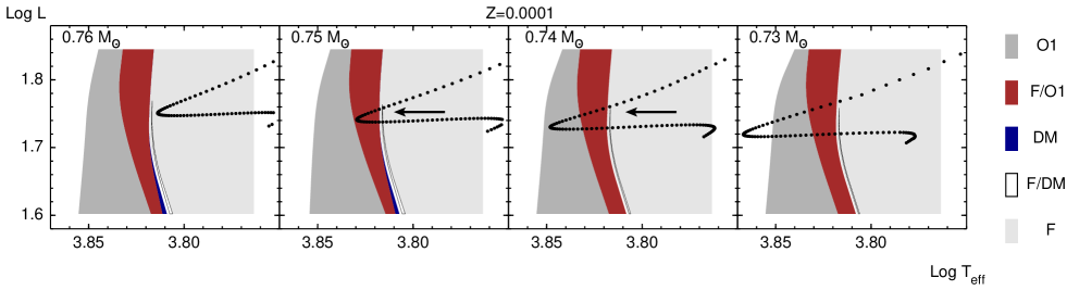
Figure 5: Demarque (demarque (2000)) evolutionary tracks superposed on modal diagram for different masses for the case of low metallicity (Z=0.0001). The plotted points denoting the evolutionary tracks are uniformly distributed in time. Color code is as in Fig. 3. F red edge is not shown. Note that for the sake of clarity the F/DM region has been plotted shifted by 100 ${{\thinspace}{\rm K}}$ to the right in the Figures. Arrows indicate the occurrence of double-mode pulsation.

5.3 The Results

Our approach provides excellent agreement between empirical and theoretical F blue edges in which previous simulations, whether radiative and convective, completely failed, mainly because they did not take into account evolutionary effects. In fact the agreement in Fig. 4. is almost perfect. It is especially striking that the overall slope of the blue edge of the F mode perfectly matches its observed counterpart, and no significant variations have been found for different evolutionary computations.

We add a note of caution however about the agreement of the locations of the F blue edges. We recall that a tuning of the dimensionless turbulent convection-related parameters results in small shifts. Therefore the almost perfect agreement for the location of the F blue edge may be a coincidence, but we stress that the slope is invariant to such changes.

Another achievement of these calculations is that the number density distribution of stars along the blue edge bears a remarkable resemblance to that of the empirical one (Fig. 1. in KBF). One notices a higher density at higher $L$, and a sparser distribution to the lower luminosity regime.

It is important to call attention to the fact that a priori  no distinct F blue edge is expected theoretically when stars with all kinds of metallicities and ages are included, and a well-mixed region is seen instead, as for Cepheids in the Magellanic Clouds (Udalski et al. Udalski (1999)).

From an observational point of view the F blue edge is equivalent to the envelope of the RRab stars. We emphasize that, because of the nature of the evolutionary tracks, from the theoretical point of view the F blue edge necessarily always means the blue edge of F/O1, and similarly, the O1 red edge is defined by the red edge of the F/O1. In Fig. 4. the F blue edge provided by our method can also be defined as the blue envelope of the F pulsators, formed through the joint effects of mode selection and evolution.

5.4 Discussion

In order to demonstrate the relevance of both mode selection and evolution in blue edge modeling, we have carried out simple tests with F/O1 edges of constant temperature, independent of ($L,M,Z$), as well as with F/O1 edges with a linear dependence on L (and independent of $M,Z$). None were successful in solving the F blue edge problem. Therefore there was no choice but to carry out all the complicated, time-consuming computations that we have just described.

Also, our earlier investigations (Szabó et al. rszabo1 (2002)) which used model sequences of only one representative metallicity, did not alter the slope significantly. The motivation for this simple treatment was the huge amount of computing capacity that was necessary to produce the diverse metallicity-sequences. We note that earlier investigations (Szabó et al. rszabo (2000)) pointed out that the shape and the location of the DMR is almost independent of $Z$, further complicating the question. It is now clear, that metallicity effects (and even the small temperature variation in IS boundaries) also play role in the correct treatment of RR Lyr ISs.

We have not considered the O1 blue edge here. Our method suggests a steeper slope compared to the F blue edge, since no hysteresis mechanism acts here. Considering O1 blue edges for fixed mass values, we can nicely reproduce other model computations (Bono et al. bono97 (1997), KBF). Thus only special distributions along the evolutionary tracks (mass, metal content and age distribution) can help to bend this slope in our framework, but we do not go into such speculations here. From an observational point of view there are too few observed stars in this region with reliable physical parameters. This prevents any meaningful comparison. Evidently future works should address this question, too.

6 Double-mode pulsation and evolution

The characteristics of the DMR have been enumerated in the discussion of the global mode selection map of Sec. 4. Here we explore an additional aspect of DM pulsation, namely its connection with stellar evolution. We have mentioned that the DMR is universally seen on the mode selection maps for all $Z$ and $L$ values. On the other hand, it is well known that RRd stars are missing from certain globular clusters (Clement et al. clement01 (2001)). We propose here that the mass distribution and stellar evolution may be the important factors involved in the resolution of this puzzle.

The DMR for a sequence of mass with fixed metallicity ($Z=0.0001$) is presented in the ${\rm Log}\thinspace{T_{\rm ef\!f}}-{\rm Log}\thinspace L$ diagram of Fig. 5. Note that again for better visibility the F/DM regions have been shifted 100 ${{\thinspace}{\rm K}}$ to the right. The bluest (interpolated) Demarque evolutionary tracks are also displayed. The arrows indicate where redward evolution cross the DMR, i.e.  where DM pulsation occurs. The Dorman models are very close to the Demarque models, at slightly lower temperatures, but the Padova tracks are much redder and do not touch our computed DMRs.

Figure 6: a.) F/O1 and DM period ratios for three luminosity and three metallicity values derived form our models. Thin lines are linear period ratios for F/O1 model sequences, (i.e. both F and O1 fixed points are nonlinearly unstable). Nonlinear period shifts from F to O1 limit cycles (or vice versa) along the separatrix (see Fig. 1a) are displayed by short vertical bars. Double-mode regions are represented by thick lines and big crosses. Models of different metallicity are separated by dotted lines. b.) Petersen diagram of all known RRd stars denoted by small triangles. The sources are the same as in Popielski et al. (popielski (2000)), complemented by Sagittarius dwarf and Galactic Bulge RRd stars from Cseresnjes (cseresnjes (2001)) and Mizerski (mizerski (2003)), as well as LMC and SMC stars from Soszynski et al. (soszynski02 (2002); soszynski03 (2003)) and Sculptor dSph RRds from Kovács (kovacs01 (2001)). The extrema of ($Z,L$) that delimit the possible DM pulsation region (taken from the left panel) are plotted to guide the eyes (dashed lines). When evolution is considered, however, the DMRs are confined to the very small trapezoids: $Z=0.0001$ at upper right, $Z=0.001$ is lower left one.

The most important feature of Fig. 5. is the narrow mass-range in which DM pulsation is possible ($M=0.745\pm 0.010\thinspace{\rm M_{\sun}}$). For $Z=0.001$ the mass range is similar, but it occurs for lower masses ($M=0.665\pm 0.010\thinspace{\rm M_{\sun}}$). With $Z=0.004$ no tracks cross the DMR. This trend is in good agreement with the results of Popielski et al. (popielski (2000)), even though they use different evolutionary and pulsational codes than we do. Their method relies on investigating the evolutionary tracks and their mapping onto a Petersen diagram. They obtain somewhat higher masses and a larger mass range ($0.79-0.855\thinspace{\rm M_{\sun}}$ with Z=0.0001, and $0.64-0.695\thinspace{\rm M_{\sun}}$ with $Z=0.001$, respectively). But, we emphasize again that we are speaking about trends, and that altering the mode selection topology by fine-tuning the turbulent parameters can lead to a wider mass-range if the DMR goes to higher $L$ e.g., or to an increase of the DM-mass by $0.01-0.02\thinspace{\rm M_{\sun}}$ if everything is shifted to lower temperatures.

According to empirical evidence the metallicity of bulge RR Lyrae ranges from $[Fe/H]=-1.5$ (0.0006) to $-0.5$ (0.006) (Walker & Terndrup wt (1991)). However the metallicity of double-mode RR Lyrae does not necessarily follow this overall metallicity distribution: First, bulge RRc stars do not show a high-metallicity tail (Walker & Terndrup wt (1991)), but a sharp cut around $[Fe/H]=-0.8$, and RRd stars presumably follow this behavior. Second, there is an immense contrast between the numbers of RRab/RRc and RRd stars: Cseresnjes (cseresnjes (2001)) found 13 galactic RRd stars among $\sim 1850$ RR Lyrae. Mizerski (mizerski (2003)) has recently found only 3 RRd stars out of 2713 bulge RR Lyrae based on OGLE-II observations. The small number of galactic bulge (and field) RRd stars inhibits the derivation of any direct connection between their metallicities and general RR Lyrae metallicity distribution. Instead, this huge difference points to the natural selection effect we propose. Moreover, all the existing metallicity estimates or measurements of RRd stars tend to low values (Clementini et al. clementini (2000), Bragaglia et al. bragaglia (2001), hereafter BGC, Kovács kovacs01 (2001)) and no bona fide high-metallicity RRd has been found to date, further supporting our findings.

We call attention to the fact that if the DMR consists of only a F/DM region then solely redward evolution can produce DM pulsation. Although we have encountered this scenario we are not in the position to exclude the possibility that blueward or both blue- and redward evolution produce DM stars. Small shifts in the locations of DM and F/DM regions or in the evolutionary tracks may change the situation. This clearly demonstrates the delicate interplay between mode selection and evolutionary effects in determining the possible parameter range of double-mode pulsation.

6.1 Petersen diagram

It is worth pointing out the fundamental difference between our theoretical Petersen diagram and previously published ones (Bono et al. bono96 (1996), Bragaglia et al. bragaglia (2001), Popielski et al. popielski (2000)). All the above works were based on F/O1 models in our notation, whereas our Petersen diagram (Fig. 6b.) consists of only DM and F/DM models. To visualize the difference, we include Fig. 6a., where both linear (and nonlinear) F/O1 and (nonlinear) DM period ratios are given without evolutionary constraints. Nonlinear period ratio shifts along the separatrix are also exhibited for selected models (see Fig. 1a). From F to O1 $P_{1}/P_{0}$ increases, from O1 to F decreases compared to its linear counterpart. These values can be important for mode switching stars at both ends of the F/O1 region. Note that DMR always follows F/O1 region at the longer period (lower temperature) side, and at higher masses (cf. Fig. 3).

The Petersen diagram supports our combined DM-pulsational and evolutionary considerations. We have plotted all the published period ratios of RRd stars in Fig. 6b. Mode selection in itself does not constrain the possible DM region as seen on panel a.) and also from the position of the dashed lines on panel b.). These lines are plotted solely for orientation, as extending the luminosity and metallicity range would further expand the permitted region. However, if evolution is taken into account, i.e. we only consider the tracks that cross the DMR, then the permitted region is approximately confined to the observed distribution on the Petersen diagram. As we have merely two metallicity values ($Z=0.0001,\ 0.001$) that are approximated by the two lozenges, we cannot reproduce the bend of the RRd star distribution, but our results are close to the observed features, though not perfect yet. We emphasize that this is the first attempt at reproducing the RR Lyr Petersen diagram on the basis of nonlinear DM models.

Another difference lies in the use of DM models only for RRd stars instead of non-DM models. Namely, as these models can be found in a much narrower region than F/O1 counterparts (Fig. 3), therefore their transformation to the Petersen diagram is also much more localized. This effect is intensified by evolutionary selection effects that lead to a shrinking of the possible DM areas, as seen in Fig. 6b. Thanks to the application of DM models and the inclusion of the evolutionary considerations, the net effects are: a.) the lifting of the persistent, disturbing mass-metallicity degeneracy and b.) the emergence of a more consistent picture, where evolutionary constraints force period ratios of the nonlinear DM-models to stretch along the observed distribution of RRd stars.

A comparison can be made with BGC published $Z=0.0001$ models (their Table 6.), which is an extension of the work described in Bono et al. (bono96 (1996)). Our F/O1 periods are quite similar (and almost parallel) to the BGC sequences. The location of our nonlinear DM (both DM and F/DM) models are somewhat different from that of the BGC models of the same $(L,M,Z)$ parameters: the $Z=0.0001$ trapezoid is at higher period ratio. The discrepancy may partly be ascribed to the fact that F/O1 regions are replaced by DMR at high masses, so the overall picture is different. A slightly smaller period ratio (by $0.001-0.002$) at this metallicity (similar that of BGC) would mean a better agreement with the observed distribution. The discussed possible shifts of the modal selection structures to higher $L$ and/or alteration of evolutionary tracks in the same sense would shift our region to the lower right, again resulting in an almost perfect explanation of the high-metallicity distribution of the observed RRd sample. In the $Z=0.001$ case either our RRd masses are too low, or a DM region being at higher temperature instead of F/DM would yield closer agreement between the observations and our predictions. Currently none of these explanations are supported by our models.

Feuchtinger (feuchtinger1 (1998)) published the first nonlinear DM model ($M=0.65M_{\sun}$, ${\rm Log}\thinspace L=1.72$, $Z=0.001$, $T_{\rm ef\!f}=6820K$, $P_{0}=0.5279$, $P_{1}/P_{0}=0.7468$). His model is at higher temperature, but the mass value perfectly agrees with ours, though no evolutionary effects were considered. Its position on the Petersen diagram disagrees with the linear and nonlinear single mode calculations and with the metallicities of the observed RRds in this region. It lies between our $Z=0.001$ and $Z=0.0001$ areas. Thus our results are closer to earlier works based on F/O1 models, such as Bono et al. (bono96 (1996)), Bragaglia et al. (bragaglia (2001)), Popielski et al. (popielski (2000)). The only possible difference between our and Feuchtinger’s code producing nonlinear DM models is a different turbulent convection parameter set. The astrophysical calibration of these parameters is still not a settled question as discussed several times throughout this paper. Interestingly, this discrepancy suggests the use of the Petersen diagram itself for the purpose of calibrating the convective parameters. An additional constraint for the models can be to ensure a good agreement with the the observed distribution on the $P_{0}-P_{1}/P_{0}$ plane, while simultaneously respecting other constraints, too (amplitudes, IS width etc.). Because of the nontrivial nature of this task and the huge amount of necessary computational time, this question is not addressed in the present work. A future work will be initiated to clear this situation.

To sum up this section, the following factors should be kept in mind when explaining the wealth of RRd stars in certain globular clusters (IC4499, M68, etc.), the low number of RRd stars in the Galactic field and other globular clusters (e.g.  M3) or even their complete absence despite the considerable abundance of RR Lyr stars:

– a very narrow mass range at a given metal content,

– a small temperature range, consequently a limited time-span for a given star,

– no high $Z$ evolutionary tracks crossing DMR.

We think that while our work is an important step in the right direction, much work remains to be done before a complete self-consistent scenario can emerge.

7 Conclusions

We have developed a very efficient methodology for studying the evolution of the pulsations of a given stellar model along its evolutionary track through the IS. It involves a judicious mixture of numerical hydrodynamics, analytical signal time-series analysis, and amplitude equations.

With the help of nonlinear, turbulent convective model computations we have analyzed in detail the modal topology of the RR Lyr IS. We have provided data on the F and O1 pulsation regimes as well as on DM regions as a function of metallicity and stellar mass. Details of the important problem of mode selection have been presented. We note that our methodology allows us to find and delineate the very narrow DM regimes very effectively, while, in contrast, with numerical hydrodynamic studies this would be akin to looking for a needle in a haystack.

Synthetic ${T_{\rm ef\!f}}-L$ diagrams of F and O1 RR Lyr stars have been generated. Toward this end we have carried out Monte-Carlo simulation for three different sets of evolutionary tracks with the purpose of deriving the RR Lyr F blue edge. The combination of numerical modeling of stellar pulsation including turbulent convection and evolutionary calculations reproduces the linear shape of the F blue edge despite the complex topology of the mode selection. We obtain essentially agreement between the empirical and the theoretical slopes, as well as for the density of stars in the IS, thus resolving an extant puzzle (KBF). It is found that observed structure of the IS can only be accounted for with a correct treatment of metallicity, mass, evolutionary effects, and nonlinear mode selection modeling. Our results provide a new, independent constraint on horizontal-branch evolution, and confirm the results of theoretical evolutionary calculations.

Based on our calculations with a large number of stars of different metallicities and masses, we find that the RRab/RRc populations are not well separated, and that there should be an area in the ${\rm Log}\thinspace{T_{\rm ef\!f}}-{\rm Log}\thinspace L$ diagram that contains both RRab and RRc stars (sometimes referred to as an either-or region).

A strong (anti-) correlation is demonstrated between the F/O1 and DM regimes. A DM region occurs at high mass, while at low mass a F/O1 region is invariably found. The transition mass between the two features depends on luminosity. Hence the simple statements that (1) RRd stars lie between the RRab and RRc pulsators, and that (2) F/O1 is between F and O1 region, can be quite misleading.

RRd stars are observed in a very narrow range of parameters (color index, temperature). On the basis of our survey we find that the possible region of DM behavior is indeed very narrow. Furthermore we show that evolution selects an even smaller region, viz.  a mass-range of extremely small width ($0.02\thinspace{\rm M_{\sun}}$) at $Z=0.0001-0.001$. The evolutionary tracks do not cross the DMR regime for high $Z$. The computed period ratios are in reasonable agreement with the observational Petersen diagram, provided that stellar evolution is taken into account. The small existing discrepancy may be ascribed to uncalibrated factors in the description of the turbulent convection, but in turn may be used to determine them.

As an extension of this work, a detailed analysis with the goal of deriving empirical relations between light-curve and physical properties of RRc stars would be of great value. Reliable light-curves (and also color-indices) of RR Lyr populations of LMC/SMC or nearby dwarf galaxies that have emerged or will emerge from large-scale surveys are bound to extend the validity of and improve the agreement between empirical and theoretical results of IS investigations.

This survey did not specifically search for second overtone pulsations, but we note that we have not encountered any RRe models. But to settle this issue, a special survey will need to be made.

- (1) Alibert, Y., Baraffe, I., Hauschildt, P. & Allard, F., 1999, A&A, 344, 551
- (2) Beaulieu, J. P., Krockenberger, M., Sasselov, D. D. et al., 1997, A&A, 321, L5
- (3) Bono, G. & Stellingwerf, R. F., 1994, ApJS, 93, 233
- (4) Bono, G., Caputo, F., Castellani, V. & Marconi, M., 1996, ApJ, 471, L33
- (5) Bono, G., Caputo, F., Castellani, V. & Marconi, M., 1997, A&AS, 121, 327
- (6) Bragaglia, A., Gratton, R. G., Carretta, E. et al., 2001, AJ, 122, 207 [BGC]
- (7) Buchler, J. R., 1993, ApSS Lib. Ser., 210, 1
- (8) Buchler, J. R. & Goupil, M. J., 1984, ApJ, 279, 394
- (9) Buchler, J. R. & Kolláth, Z., 2002, ApJ, 573, 324 [BK2002]
- (10) Buchler, J. R & Kovács, G., 1986, ApJ, 308, 661
- (11) Buchler, J. R. & Kovács, G., 1987, ApJ, 318, 232
- (12) Castellani, M., Caputo, F. & Castellani, V., 2003, A&A, 410, 871
- (13) Catelan, M., 2004, ApJ, 600, 409
- (14) Clement, C. M., Muzzin, A., Dufton, Q. et al., 2001, AJ, 122, 2587
- (15) Clementini, G., Di Tomaso, S., Di Fabrizio, L. et al. 2000, AJ, 120, 2054
- (16) Cohen, L., 1994, Time-Frequency Analysis. Prentice-Hall PTR. Englewood Cliffs, NJ
- (17) Cseresnjes, P., 2001, A&A, 375, 909
- (18) Demarque, P., Zinn, R., Lee, Y-W. & Yi, S., 2000, AJ, 119, 1398
- (19) Dorfi, E. A. & Feuchtinger, M. U., 1999, A&A, 348, 815
- (20) Dorman, B., 1992, ApJS, 81, 221
- (21) Feuchtinger, M. U., 1998, A&A, 337, 29
- (22) Gábor, D., 1946, Theory of communications, J.IEEE (London), 93, 429
- (23) Gallart, C., Zoccali, M., Bertelli, G. et al., 2003, AJ, 125, 742
- (24) Girardi, L., Bressan, A., Bertelli, G. & Chiosi, C., 2000, A&AS, 141, 371
- (25) Jackson, J. D., 1975, Classical Electrodynamics, J. Wiley, NY
- (26) Jurcsik, J., 1997, Poster Vol. of the IAU Symp. No. 181. , 261 Eds.: Schmider, F. X. and Provost, J.
- (27) Jurcsik, J., 1998, A&A, 333, 571
- (28) Kolláth, Z., Beaulieu, J. P., Buchler, J. R. & Yecko, P., 1998, ApJ, 502, L55
- (29) Kolláth, Z. & Buchler, J. R., 2001, ApSS Lib. Ser., 257, 29
- (30) Kolláth, Z., Buchler, J. R. & Feuchtinger, M., 2000, ApJ, 540, 468 [KBF]
- (31) Kolláth, Z., Buchler, J. R., Szabó, R. & Csubry, Z., 2002, A&A, 385, 932 [KBSC]
- (32) Kovács, G., 2001, A&A, 375, 469
- (33) Kovács, G. & Buchler, J. R., 1993, ApJ, 404, 765
- (34) Kovács, G., Buchler J. R. & Davis, C. G., 1987, ApJ, 319, 247
- (35) Kovács, G. & Jurcsik, J., 1996, ApJ, 466, L17
- (36) Kovács, G. & Jurcsik, J., 1997, A&A, 322, 218
- (37) Lee, Y.-W., Demarque, P. & Zinn, R., 1994, ApJ, 423, 248
- (38) Mizerski, T., 2003, Acta Astron., 53, 307
- (39) Popielski, B. L., Dziembowski, W. A. & Cassisi, S., 2000, Acta Astron. 50, 491
- (40) Schaller, G. Schaerer, D. Meynet, G. & Maeder, A., 1992, A&AS, 96, 269
- (41) Szabó, R., Csubry, Z., Kolláth, Z. & Buchler, J. R., 2000, ASP Conf. Ser., 203, 374
- (42) Szabó, R., Csubry, Z., Kolláth, Z. & Buchler J. R., 2002, ASP Conf. Ser., 259, 404
- (43) Soszynski, I., Udalski, A., Szymanski, M. et al., 2002, Acta Astron., 52, 369
- (44) Soszynski, I., Udalski, A., Szymanski, M. et al., 2003, Acta Astron., 53, 93
- (45) Udalski, A., Soszynski, I., Szymanski, M. et al., 1999, Acta Astron., 49, 1
- (46) van Albada, T. S. & Baker N., 1973, ApJ, 185, 477
- (47) Walker, A. R. & Terndrup, D. M., 1991, ApJ, 378, 119
- (48) Yecko, P. A., Kolláth, Z. & Buchler, J. R., 1998, A&A, 336, 553