First observation of Jupiter by XMM-Newton

We present the first X-ray observation of Jupiter by XMM-Newton. Images taken with the EPIC cameras show prominent emission, essentially all confined to the 0.2$-$2.0 keV band, from the planet’s auroral spots; their spectra can be modelled with a combination of unresolved emission lines of highly ionised oxygen (OVII and OVIII), and a pseudo-continuum which may also be due to the superposition of many weak lines. A 2.8$\sigma$ enhancement in the RGS spectrum at 21$-$22 Å ($\sim$0.57 keV) is consistent with an OVII identification. Our spectral analysis supports the hypothesis that Jupiter’s auroral emissions originate from the capture and acceleration of solar wind ions in the planet’s magnetosphere, followed by X-ray production by charge exchange. The X-ray flux of the North spot is modulated at Jupiter’s rotation period. We do not detect evidence for the $\sim$45 min X-ray oscillations observed by Chandra more than two years earlier. Emission from the equatorial regions of the planet’s disk is also observed. Its spectrum is consistent with that of scattered solar X-rays.

1 Introduction

Jovian auroral X-ray emissions were first observed with the Einstein Observatory (Metzger et al. Metzger (1983)) and were extensively studied with ROSAT (e.g. Waite et al. Waite94 (1994), Gladstone et al. Gladstone98 (1998)), which provided limited spectral information but fairly extensive imaging data. The emissions have been explained as the result of charge exchange and excitation of energetic ($>$1 MeV per nucleon) S and O ions (Cravens et al. Cravens (1995), Cravens03 (2003)). The ions were first thought to originate in Io’s volcanos, and to precipitate from a region of Jupiter’s magnetosphere just outside the Io Plasma Torus (IPT) at about 8 – 12 Jovian radii (Mauk et al. Mauk (1996)). This idea had to be reconsidered, though, because of more recent (December 2000) Chandra observations: they have shown that most of Jupiter’s northern auroral X-rays come from a hot spot located poleward of the latitudes connected to the inner magnetosphere, pointing to a particle population in the outer magnetosphere beyond 30 Jovian radii (Gladstone et al. Gladstone02 (2002)). The magnetic mapping of the hot spot to such large distances presents serious difficulties regarding the source of the precipitating particles, since at $>$30 Jovian radii there are insufficient S and O ions to account for the hot spot emissions. Lack of correlation between the X-ray emission morphology and the surface magnetic field strength also suggests that some process other than energetic ion precipitation from the inner magnetosphere is responsible for the bulk of the auroral X-rays. One possibility is high-latitude reconnection of the planetary and solar wind magnetic fields, with the subsequent entry of the highly ionised (but low energy) heavy ion component (such as highly charged O, Fe, etc.) of the solar wind. The ions could then be accelerated to MeV energies by the currents present in the outer magnetosphere, thereby producing a spectrum rich in emission features much like comets. Indeed Chandra ACIS-S spectra (Elsner et al. 2004, in preparation) indicate a role for energetic O and S ion precipitation as a source of the X-ray aurora: they show a strong OVIII line at 653 eV, which puts the charge exchange X-ray production, pioneered by Horanyi et al. (Horanyi (1988)) and Cravens et al. (Cravens (1995)), on firm observational ground.

Another intriguing aspect of Jupiter’s hot spot X-ray emissions observed by Chandra in December 2000 are $\sim$45 min pulsations, similar to those reported for high-latitude radio and energetic electron bursts observed by the Ulysses spacecraft during a fly-by a decade before (MacDowall et al. MacDowall (1993), McKibben et al. McKibben (1993)). However, no comparable periodicity was seen in solar wind or interplanetary magnetic field measurements made by Cassini upstream of Jupiter at the time of the Chandra observations in 2000, indicating that the pulsations must arise from processes internal to the Jovian magnetosphere,

In addition, there is the open question of the source of Jupiter’s low-latitude X-rays. Maurellis et al. (Maurellis (2000)) have recently suggested that much of the equatorial X-ray emission can be understood by the scattering of solar X-ray photons by Jupiter’s atmosphere. However, Waite et al. (Waite97 (1997)) argued that the correspondence between the low-latitude surface magnetic field and the observed longitudinal asymmetries in the X-ray emission observed by ROSAT can best be explained by energetic S and O ion precipitation from the inner radiation belts.

We set out to use the unparalleled combination of grasp and energy resolution of the XMM-Newton payload to investigate some of the un-answered questions concerning Jupiter’s X-ray emission. Reported here is the initial 110 ks observation performed in April 2003: its primary aim was that of verifying the feasibility of pointing at an optically bright target such as Jupiter. A more recent, longer (245 ks) XMM-Newton observation carried out in November 2003 will be presented in a future publication.

2 Observations

XMM-Newton (Jansen et al. Jansen (2001)) observed Jupiter for 110 ks between 2003, April 28, 16:00 and April 29, 22:00. The EPIC-MOS (Turner et al. turner (2001)) and pn (Strüder et al. struder (2001)) cameras (with a field of view of 30′ diameter) were operated in Full Frame and Large Window mode respectively, and the RGS instrument (den Herder et al. denHerder (2001)) in Spectroscopy. The filter wheel of the OM telescope (Mason et al. Mason (2001)) was kept in the BLOCKED position because the optical brightness of Jupiter is above the safe limit for the instrument, so no OM data were collected; also to minimise the risk of optical contamination the EPIC cameras were used with the thick filter. For a solar-type spectrum this filter is able to suppress efficiently the optical contamination for point sources up to magnitude 0 (pn) and 1 (MOS); this is valid for the worst case, of the brightest pixel within the core of the Point Spread Function (PSF), and for Full Frame operational modes. During the April 2003 XMM-Newton observation Jupiter had a surface brightness of 5.5 mag/arcsec² (from the JPL HORIZONS Ephemeris Generator). Thus we do not expect optical contamination in the EPIC-MOS cameras (1.1″ $\times$ 1.1″ pixels) nor in the pn (4.1″ $\times$ 4.1″ pixels). This is confirmed by the lack of evidence for a steep rise in the spectra towards the lowest energies (see Fig.s 6, 7 and  8).

Jupiter’s motion on the sky (11″/hr) required eight pointing trims during the long observation in order to avoid worsening the RGS spectral resolution; the planet’s path was very close to the RGS dispersion direction, so that the RGS spectra of Jupiter’s two poles, well separated spatially (the planet’s disk diameter was 38″ during the observations), did not overlap.

The data were analysed with the XMM-Newton Science Analysis Software (SAS) v. 5.4 (see SAS User’s Guide at http:// xmm.vilspa.esa.es/external/xmm_user_support/documentation). Photons collected during the nine pointings along Jupiter’s path were referred to the centre of the planet’s disk. An image of the planet, obtained by combining EPIC-pn, MOS1 and MOS2 data, is shown in Fig. 1. A field source was occulted by Jupiter’s equatorial region at the beginning of the observation: because of its low countrate (one fifth of the planet’s disk) and of the short time ($\sim$1 hr) for eclipse ingress and egress, the source is expected to produce no contamination on Jupiter’s equatorial emission.

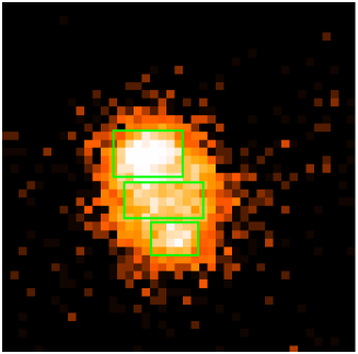
Figure 1: Jupiter’s image (2′ side) obtained combining EPIC-pn, MOS1 and MOS2 data; North is to the top and East to the left. Superposed are the rectangular regions used in the extraction of auroral and disk lightcurves and spectra.

The top panel of Fig. 2 shows the EPIC-pn lightcurve (100 s bins) for the full camera at energies $>$ 10 keV, which gives a good indication of the temporal behaviour of the particle background. Beginning and end of the observation are affected by higher background levels; excluding such times, a low-background period of 80 ks (2003, April 28, 19:07 $-$ April 29, 17:20) is available and further analysis was restricted to this.

Figure 2: EPIC-pn lightcurves from the observation of Jupiter (Top panel: full camera field at energies $>$ 10 keV, in 100 s bins, showing times of high particle background; middle panels: 0.2$-$2.0 keV, 200 s bins; bottom panel: Central Meridian Longitude; see text for details).

3 EPIC timing analysis

When extracting lightcurves (and spectra; see Sect. 4) for the auroral regions we have taken into account the fact that the XMM-Newton telescope PSF will ’mix’ the auroral events with some from the planet’s disk. In order to establish the amount of such contamination we convolved Chandra ACIS images (PSF of about 0.8″ Half Energy Width, or HEW) with the XMM-Newton telescope PSF ($\sim$15″ HEW), and estimated the percentages of auroral, disk and off-planet diffuse background events falling in rectangular regions of different sizes positioned at the auroral spots. As extraction regions we selected larger rectangles (24″ x 16″ for the North spot and 16″ x 12″ for the South) in preference to smaller ones because they allow us to include a larger number of auroral photons, with only a relatively small increase in the contributions of disk and background events. A rectangular box (28″ $\times$ 13″) was also used to extract Jupiter’s equatorial lightcurve and spectrum. The extraction regions are shown in Fig. 1, superposed on the combined EPIC-pn, MOS1 and MOS2 image of Jupiter: we expect that in the boxes over the North and South spots 71 and 66% of the events are of auroral origin, 27 and 31% of disk origin, and 2 and 3% are from the off-planet diffuse background, respectively. The latter contribution is small enough that it was neglected when extracting the auroral lightcurves (and spectra). A $\sim$2% contribution of particle background (estimated from an out-of-field-of-view area of the MOS1 camera) was also neglected.

EPIC-pn lightcurves for Jupiter’s equatorial region and the planet’s North and South auroral spots (the latter two after subtraction of the appropriate contribution from Jupiter’s disk) are shown in the middle panels of Fig. 2 (in 200 s bins and in the energy range 0.2$-$2.0 keV, where essentially all the X-ray emission is detected).

The planet’s $\sim$10 hr rotation period is clearly seen in the lightcurve of the North spot (third panel from top in Fig. 2), but is apparently not visible for the (weaker) South spot (bottom but one panel) and the equatorial region (second panel from top). We have further investigated the possible presence of periodic variability in the X-ray emissions of Jupiter by generating amplitude spectra for the lightcurves (in 240 s bins) of the events originating in the equatorial and the two auroral regions individually.

The amplitude spectra (Fig. 3) clearly show power at Jupiter’s 10 hr rotation period in the North spot, but not in the South spot nor in the equatorial data. This is confirmed by inspection of the lightcurves folded on the 10 hr period (Fig. 4).

Figure 3: EPIC-pn amplitude spectra for Jupiter’s North and South spots and equatorial region.

Figure 4: EPIC-pn lightcurves folded on Jupiter’s 10 hr rotation period.

The bottom panel in Fig. 2 shows the Central Meridian Longitude (CML, i.e. the system III longitude of the meridian facing the observer) for the duration of the XMM-Newton observation. From the plot it is clear that the North spot is brightest around longitude 180°, which is similar to what Chandra found (Gladstone et al. Gladstone02 (2002)); for the equatorial region and the South spot the distribution in longitude is more or less uniform (again similar to Chandra, which revealed a band, rather than a hot spot, of emission near the South pole).

A search for periodic behaviour at shorter timescales (e.g. the $\sim$45 min oscillations observed by Chandra in December 2000) shows that there are individual peaks in the power spectrum below 200 min (see Fig. 3), but that they are not significant: we proved this by taking the N spot lightcurve, randomly populating the data bins (of 240 s each) and generating the events amplitude spectra. This was repeated 100 times, with the result that no peak in the observed data is greater than the general noise in the simulated data. A separate power spectrum analysis of the section of the lightcurve between 2$\times 10^{4}$ and 4$\times 10^{4}$ s into the observation (which shows a ’burst’-type behaviour) also does not produce any significant peak. Amplitude analysis of the EPIC-MOS data produces results consistent with those from the pn.

We conclude that the $\sim$45 min oscillations observed by Chandra in December 2000 were not present, or were below the level of detectability, during the XMM-Newton observation of April 2003. It is worth pointing out that subjecting the XMM-Newton data to the same analysis carried out on the Chandra data shows a very similar level of amplitude noise at periods shorter than $\sim$30 min.

4 EPIC spectral analysis

Fig. 5 shows a smoothed EPIC-pn colour image of Jupiter (where red corresponds to 0.2$-$0.5 keV, green to 0.5$-$0.7 keV and blue to 0.7$-$2.0 keV) which clearly demonstrates that the equatorial disk emission is harder than that of the auroral spots.

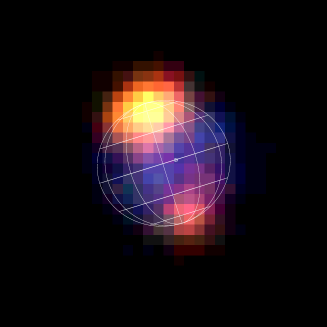
Figure 5: Smoothed EPIC-pn image of Jupiter (2.9″ pixels); North is to the top and East to the left; colour code: red - 0.2$-$0.5 keV, green - 0.5$-$0.7 keV, blue - 0.7$-$2.0 keV. A graticule showing Jupiter’s orientation with 30° intervals in latitude and longitude is overlaid. The circular mark indicates the sub-solar point; the sub-Earth point is at the centre of the graticule.

EPIC-pn, MOS1 and 2 spectra for Jupiter’s auroral spots and disk were extracted using the SAS task xmmselect, selecting only good quality (FLAG = 0) events. The appropriate percentage of disk events (see Sect. 3) was then subtracted from the auroral spectra, after normalising to the different areas of the extraction regions. No background was subtracted from the disk spectrum. The resulting spectra were combined to produce integrated EPIC spectra for the North and South spots and the equatorial disk region; finally the spectra were binned so as to have a S/N ratio greater than 3$\sigma$ (North spot) or at least 20 counts (South spot and equator) in each bin: in this way the $\chi^{2}$ minimisation technique is applicable in the fits. The spectra were fitted, using XSPEC v. 11.3.0, in the energy range 0.2$-$2 keV, which contains essentially all the signal from Jupiter. Response matrices and auxiliary response files for the three EPIC cameras and each of Jupiter’s three regions were built using the SAS tasks rmfgen and arfgen. Since most or all of the flux comes from inside the extraction boxes and there is no source flux from outside the boxes falling into them, we adopted the point source option in arfgen, because this will produce a better approximation of the real flux. The response matrices for the three EPIC cameras were then combined (following Page et al. Page (2003)) before being convolved with the spectral models in the fitting procedure for each region of the planet.

4.1 North and South auroral spots

A mekal coronal plasma model and models comprising a number of Gaussian emission lines, with and without a continuum component, were tried.

The best mekal fits to the auroral regions are obtained for a temperature of $\sim$0.2 keV with solar abundances, but the values of $\chi^{2}$/d.o.f. are very high (106/44 and 59/25 for the North and South spots respectively): the overall shape of the model is a poor match to the observed spectrum and the sharp peak at $\sim$0.6 keV. For both auroral regions the best fit ($\chi^{2}$/d.o.f. = 46/40 and 20/21 for North and South spot respectively) is found with a power law continuum and five Gaussian emission lines corresponding to CVI Ly$\alpha$ (0.37 keV), the OVII triplet (0.57 keV), OVIII Ly$\alpha$ (0.65 keV), a combination of higher order OVII transitions (effective energy 0.69 keV) and a blend of higher order OVIII lines (effective energy 0.80 keV). The energies of the lines were fixed in the fits and their intrinsic widths were set to zero (the latter are found to be below the EPIC resolution, or consistent with zero, if they are allowed to vary in the fits).

The relevant best fit parameters (with errors; these are quoted at 90% confidence throughout the paper) are given in Table 1; data, best fit model and the contribution of each bin to the $\chi^{2}$ are shown in Fig. 6 and Fig. 7 for the North and the South spot respectively. The measured 0.3$-$2.0 keV flux is 5.6 $\times$ 10^-14 erg cm^-2 s^-1 for the North spot, and 2.1 $\times$ 10^-14 erg cm^-2 s^-1 for the South.

Figure 6: Data and best fit for the EPIC-pn spectrum of Jupiter’s North auroral spot (see text for details).

Figure 7: Data and best fit for the EPIC-pn spectrum of Jupiter’s South auroral spot (see text for details).

Figure 8: Data and best fit for the EPIC-pn spectrum of Jupiter’s equatorial region (see text for details).

Table 1: Best fit parameters for the 0.2$-$2 keV spectra of Jupiter’s auroral spots (errors are at 90% confidence).

$\begin{array}[]{lccccc}\hline\cr\hline\cr\vskip 3.0pt plus 1.0pt minus 1.0pt\cr&&\lx@intercol\hfil North\leavevmode\nobreak\ spot\hfil\lx@intercol&\lx@intercol\hfil South\leavevmode\nobreak\ spot\hfil\lx@intercol\\ &&\Gamma^{a}&Norm^{b}&\Gamma^{a}&Norm^{b}\\ \vskip 3.0pt plus 1.0pt minus 1.0pt\cr\hline\cr\vskip 3.0pt plus 1.0pt minus 1.0pt\cr Power\leavevmode\nobreak\ law&&3.23^{\rm+0.20}_{\rm-0.25}&4.59^{\rm+0.66}_{\rm-0.69}&2.68^{\rm+0.53}_{\rm-0.38}&3.02^{\rm+0.63}_{\rm-0.71}\\ \vskip 3.0pt plus 1.0pt minus 1.0pt\cr\hline\cr\vskip 3.0pt plus 1.0pt minus 1.0pt\cr Emiss.\leavevmode\nobreak\ lines&Energy^{c}&Flux^{d}&EW^{e}&Flux^{d}&EW^{e}\\ \vskip 3.0pt plus 1.0pt minus 1.0pt\cr\hline\cr\vskip 3.0pt plus 1.0pt minus 1.0pt\cr CVI\leavevmode\nobreak\ Ly\alpha\nobreak\leavevmode&0.37&14.28^{\rm+5.18}_{\rm-5.13}&130^{\rm+47}_{\rm-47}&3.89^{\rm+3.57}_{\rm-3.78}&88^{\rm+81}_{\rm-86}\\ \vskip 3.0pt plus 1.0pt minus 1.0pt\cr OVII\leavevmode\nobreak\ triplet\nobreak\leavevmode&0.57&17.69^{\rm+2.54}_{\rm-2.33}&638^{\rm+92}_{\rm-84}&4.30^{\rm+1.71}_{\rm-1.59}&305^{\rm+121}_{\rm-113}\\ \vskip 3.0pt plus 1.0pt minus 1.0pt\cr OVIII\leavevmode\nobreak\ Ly\alpha&0.65&1.54^{\rm+1.45}_{\rm-1.29}&85^{\rm+56}_{\rm-71}&0.93^{\rm+1.26}_{\rm-0.93}&110^{\rm+149}_{\rm-110}\\ \vskip 3.0pt plus 1.0pt minus 1.0pt\cr OVII\leavevmode\nobreak\ higher\nobreak\leavevmode&0.69&3.42^{\rm+1.02}_{\rm-0.96}&228^{\rm+68}_{\rm-64}&0.97^{\rm+0.83}_{\rm-0.97}&94^{\rm+80}_{\rm-94}\\ \vskip 3.0pt plus 1.0pt minus 1.0pt\cr OVIII\leavevmode\nobreak\ higher\nobreak\leavevmode&0.80&1.68^{\rm+0.64}_{\rm-0.60}&180^{\rm+69}_{\rm-64}&0.82^{\rm+0.55}_{\rm-0.57}&144^{\rm+97}_{\rm-100}\\ \vskip 3.0pt plus 1.0pt minus 1.0pt\cr\hline\cr\hline\cr\end{array}$

^a Photon index
^b Power law normalisation at 1 keV in units of 10^-6 ph cm^-2 s^-1 keV^-1
c Energy of the emission features in keV (fixed in the fits)
^d Total flux in the line in units of 10^-6 ph cm^-2 s^-1
e Line equivalent width in eV

We explored the possibility that CV (0.31 keV) rather than CVI emission may be present at the low energy end of the spectra by letting the energy of the line free in the fits: for the North spot we find a best fit energy of 0.36$\pm$0.02 keV ($\chi^{2}$/d.o.f. = 45/39); fixing the line at 0.31 keV gives a much worse fit with $\chi^{2}$/d.o.f. = 53/40. For the South spot, the best fit energy is 0.33${}^{\rm+0.02}_{\rm-0.03}$ ($\chi^{2}$/d.o.f. = 17/20), marginally consistent with CV emission; the rather poor statistical quality of the data, though, makes line discrimination uncertain.

With a view at establishing the origin (solar wind or inner magnetosphere) of the ions responsible for the X-ray production in the auroral spots, we checked whether the carbon emission could be replaced by sulphur lines: we considered lines (or blends) at 0.32 keV (SXI), 0.34 keV (SXII) and 0.35 keV (SXIII) (some of the strongest in the atomic spectral tables of Podobedova et al. Podo (2003); see also Elsner et al. 2004, in preparation). While the energy resolution of the EPIC CCDs ($\sim$100 eV FWHM below 1 keV), combined with the low countrate, make it very hard to distinguish between lines that are so close in energy, the best fits obtained by letting the line energy free (see above) appear to indicate, at least for the North spot, preference for a higher energy, i.e for the CVI Ly$\alpha$ line (0.37 keV).

We find similar line intensities to those listed in Table 1, but slightly worse fits, if we substitute a bremsstrahlung continuum for the power law ($\chi^{2}$/d.o.f. = 48/40 and 25/21 for North and South spot respectively). Replacing the continuum component with a combination of emission lines also produces worse quality fits.

4.2 Equatorial region

As suggested by Fig. 5, we find that Jupiter’s equatorial region displays a different, harder spectrum than the auroral spots. The data are best fitted ($\chi^{2}$/d.o.f. = 26/38) by a two temperature mekal model, with solar abundances, combined with a bremsstrahlung continuum and a Gaussian emission line at 1.35 keV (fixed in the fit), corresponding to the energy of the MgXI triplet. Relevant best fit parameters are listed in Table 2; data, best fit model and $\chi^{2}$ contribution from each spectral bin are shown in Fig. 8. A fit of the same statistical quality is obtained replacing the bremsstrahlung component with a power law of photon index 1.37 and normalisation at 1 keV of 1.46 $\times$ 10^-6 ph cm^-2 s^-1 keV^-1. The 0.3$-$2.0 keV flux measured for the equatorial region is 4.0 $\times$ 10^-14 erg cm^-2 s^-1.

Table 2: Best fit parameters for the 0.2$-$2 keV spectrum of Jupiter’s equatorial region (errors are at 90% confidence)

$\begin{array}[]{lccccc}\hline\cr\hline\cr\vskip 3.0pt plus 1.0pt minus 1.0pt\cr&&\lx@intercol\hfil Equator\hfil\lx@intercol\\ &&kT_{1}^{a}&Norm^{b}&kT_{2}^{a}&Norm^{b}\\ \vskip 3.0pt plus 1.0pt minus 1.0pt\cr\hline\cr\vskip 3.0pt plus 1.0pt minus 1.0pt\cr{\tt mekal}&&0.13^{\rm+0.04}_{\rm-0.02}&11.0^{\rm+5.89}_{\rm-5.18}&0.44^{\rm+0.06}_{\rm-0.06}&9.08^{\rm+1.66}_{\rm-1.54}\\ \vskip 3.0pt plus 1.0pt minus 1.0pt\cr Bremsstrahlung&&5^{\rm+136}_{\rm-4}&2.07^{\rm+2.34}_{\rm-0.97}&&\\ \vskip 3.0pt plus 1.0pt minus 1.0pt\cr\hline\cr\vskip 3.0pt plus 1.0pt minus 1.0pt\cr Emiss.\leavevmode\nobreak\ line&Energy^{c}&Flux^{d}&EW^{e}&&\\ \vskip 3.0pt plus 1.0pt minus 1.0pt\cr\hline\cr\vskip 3.0pt plus 1.0pt minus 1.0pt\cr MgXI&1.35&0.39^{\rm+0.21}_{\rm-0.22}&144^{\rm+78}_{\rm-81}&&\\ \vskip 3.0pt plus 1.0pt minus 1.0pt\cr\hline\cr\hline\cr\end{array}$

^a mekal/bremsstrahlung temperature in keV
^b mekal/bremsstrahlung normalisation in units of 10^-6 ph cm^-2 s^-1 keV^-1
c Energy of the emission feature in keV (fixed in the fits)
^d Total flux in the line in units of 10^-6 ph cm^-2 s^-1
e Line equivalent width in eV

5 RGS detection

The data from RGS1 and RGS2 (cross-dispersion vs dispersion, before background subtraction, 1st order only) are shown as colour plots in the top panels of Fig. 9, and the extracted 1st order spectra, background-subtracted, are in the middle panels. The gross spectrum of the planet is obtained by integrating along the cross-dispersion direction within $\pm$40″ of the centre of the planet’s disk (i.e. between the two darker horizontal lines in the top panels of Fig. 9). The background spectrum is the sum of two slices, each 40″ wide, centred at $\pm$62″ from the centre of the planet’s disk (i.e. in practice between the darker and the lighter horizontal lines in Fig. 9).

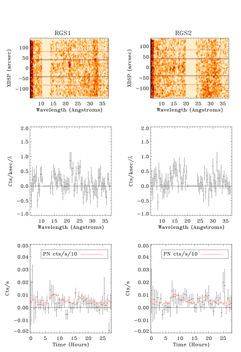
Figure 9: Top: RGS1 (left) and 2 (right) cross-dispersion vs dispersion plots for the Jupiter observation; the cross-dispersion scale is referred to the centre of the planet’s disk. Middle: RGS1 (left) and 2 (right) background-subtracted spectra. Bottom: RGS1 (left) and 2 (right) lightcurves, with the EPIC-pn lightcurve, appropriately scaled, superposed (in red).

It is tantalising to see a bright spot at the expected location of the OVII triplet (21–22 Å, or $\sim$0.57 keV) in the RGS1 colour plot, at the expected location of the North auroral spot (just above the origin in the cross-dispersion direction, which corresponds to the centre of the planet’s disk). There appears to be an enhancement also at about 15 Å in RGS2, practically at the centre in the cross-dispersion direction, implying a lower latitude on the planet. However, it has to be stressed that these are very low surface brightness features, which only a longer observation will be able to confirm.

In order to quantify the possible OVII detection, a box of  40″ in the cross-dispersion direction and 5 resolution elements ($\sim$0.3 Å) in the dispersion direction was used to measure the general level of background over CCD4 and the excess at the expected location of OVII: this results in a 2.8$\sigma$ excess in the box centred on OVII. A similar estimate is obtained for the excess around 15 Å in RGS2.

The bottom panels in Fig. 9 show the background subtracted RGS lightcurves with the 0.2 – 2 keV EPIC-pn lightcurves superposed, appropriately scaled: the good match of the data from the two instruments adds credibility to the possible detection of Jupiter X-rays in the RGS.

6 Discussion and conclusions

The first XMM-Newton observation of Jupiter provides interesting new information with which we can try and clarify some of the many unresolved issues concerning the planet’s X-ray emission. Here we consider some of them.

i) The XMM-Newton EPIC spectra of the North and South auroral regions of Jupiter can be explained as the superposition of emission lines from highly ionised oxygen and carbon (the latter in preference to sulphur, at least for the North spot). The power law component which is also needed to model the spectra could be a pseudo-continuum produced by the combination of weaker discrete emission features (although our attempts at replacing the power law with a combination of emission lines did not formally improve the quality of the fits). A spectrum consisting of many unresolved lines (mostly due to OVII and OVIII ions) was found to provide the best fit to the Chandra data of comet McNaught-Hartley and was interpreted as the result of electron capture by heavy ions of the solar wind colliding with the cometary atmosphere (Kharchenko et al. khar (2003)). A similar interpretation can be proposed for Jupiter’s auroral spots: solar wind ions could be captured and accelerated in the planet’s magnetic field, and subsequent charge exchange would lead to the observed spectra, rich in line emission from highly ionised oxygen and carbon. The identification of a CVI rather than CV transition (Sect. 4) would also support an origin from the solar wind, in which carbon is usually fully ionised.

The North and South spot EPIC spectra (together with the tentative detection in RGS) clearly show a larger contribution from OVII line emission, relative to OVIII; this contrasts with what has been reported from Chandra observations in February 2003 (Elsner et al. 2004, in preparation) and suggests variability, over a period of a few weeks, in the level of ionisation, and thus of overall energy of the ions penetrating Jupiter’s upper atmosphere.

ii) The 0.3$-$2.0 keV fluxes derived from the above spectral analysis correspond to X-ray luminosities of 0.43, 0.16 and 0.31 GW for Jupiter’s North and South spots, and equatorial region respectively. Thus the XMM-Newton results for the auroral regions are in good agreement with those of Chandra two months earlier (February 2003): at this time Elsner et al. (Elsner (2003)) measured a countrate roughly half of what was observed in December 2000 (Gladstone et al. Gladstone02 (2002)), when the 0.3$-$2.0 keV luminosities of North and South spots, and of the equatorial region were 1.0, 0.4 and 2.3 GW respectively. The disk measurement by XMM-Newton appears to be significantly lower than the Chandra one: the difference may be due to the use of different extraction regions for the disk emission.

iii) The planet’s 10 hr rotational period is observed to modulate the emission of only the North polar spot, which is found to be at a similar system III longitude ($\sim$180°) as in the Chandra observations of December 2000. If modulation is present in the South spot, it must be at a much lower level than observed with Chandra.

Chandra images have been used to establish that the North and South spots have different morphological appearances, with the North spot well localised and the South extended into a band (Elsner et al. Elsner (2003)). It is difficult to comment on this with our data, because the XMM-Newton spatial resolution is poorer than that of Chandra. However, different morphologies, combined with inclination effects, may be able to explain the different temporal behaviours at the two poles.

iv) There is no evidence in the XMM-Newton data for the $\sim$45 min oscillations observed with Chandra in December 2000. This is consistent with Chandra’s non-detection in February 2003 and the lack of radio quasi-periodic oscillations in Ulysses data at the same time (Elsner et al. 2004, in preparation). We conclude that the oscillations must be a transient phenomenon, possibly related to magnetospheric effects on Jupiter, which could be variable as a consequence of solar wind variability.

v) Jupiter’s equatorial X-ray spectrum is harder than that of the polar regions and resembles what is expected from the scattering of solar X-rays, in keeping with the prediction of Maurellis et al. (Maurellis (2000)): a two-temperature coronal plasma is required to fit the spectrum, as well as a contribution from Mg line emission. The latter may be simply reflected sunlight. Interestingly, a similar feature at $\sim$1.4 keV is apparent in the XMM-Newton spectrum of Saturn (Ness et al. NessX (2004)). The bremsstrahlung component in Jupiter’s spectrum has an unrealistically high temperature (with very large errors) and is likely to indicate again the presence of a low level residual flux which could be due to the superposition of weaker, unresolved lines.

In general Jupiter’s equatorial X-ray emission appears to show characteristics similar to those observed with XMM-Newton and Chandra for Saturn’s disk emission (Ness et al. NessX (2004), 2004a ), which can also be modelled with a coronal plasma and line emission (likely to be from oxygen). However, no bright auroral emission is observed on Saturn, at least from the South pole (which was the only pole visible during the Chandra observation), suggesting different conditions in the magnetospheres of the two planets.

- (1) Cravens, T. E., Howell, E., Waite, J. H., Jr., & Gladstone, G. R. 1995, J. Geophys. Res., 100, 17153
- (2) Cravens, T. E., Waite, J. H., Jr., Gombosi, T. I. et al.. 2003, J. Geophys. Res., 108, 1465
- (3) den Herder, J. W., Brinkman, A. C., Kahn, S. M. et al. 2001, A&A, 365, L7
- (4) Elsner, R., Gladstone, R., Waite, H. et al. Poster at the ’Four Years of Chandra Observations’ Symposium, Huntsville, Alabama, USA, October 2003
- (5) Gladstone, G. R., Waite, J. H., Jr. & Lewis, W. S. 1998, J. Geophys. Res., 103, 20083
- (6) Gladstone, G. R., Waite, J. H., Jr., Grodent, D. et al. 2002, Nat, 415, 1000
- (7) Horanyi, M., Cravens, T. E. & Waite, J. H., Jr. 1988, J. Geophys. Res., 93, 7251
- (8) Jansen, F., Lumb, D., Altieri, B. et al. 2001, A&A, 365, L1
- (9) Kharchenko, V., Rigazio, M, Dalgarno, A. & Krasnopolsky, V. A. 2003, ApJ, 585, L73
- (10) MacDowall, R. J., Kaiser, M. L., Desch, M. D. et al. 1993, Planet. Space Sci., 41, 1059
- (11) Mason, K. O., Breeveld, A., Much, R. et al. 2001, A&A, 365, L36
- (12) Mauk, B. H., Gary, S. A., Kane, M. et al. 1996, J. Geophys. Res., 101, 7685
- (13) Maurellis, A. N., Cravens, T. E., Gladstone, G. R. et al. 2000, Geochim. Res. Lett., 27, 1339
- (14) McKibben, R. B., Simpson, J. A. & Zhang, M. 1993, Planet. Space Sci., 41, 1041
- (15) Metzger, A. E., Luthey, J. L., Gilman, D. A. et al. 1983, J. Geophys. Res., 88, 7731
- (16) Ness, J.-U., Schmitt, J. H. M. M. & Robrade, J. 2004, A&A, 414, L49
- (17) Ness, J.-U., Schmitt, J. H. M. M., Wolk, S. J., Dennerl, K. & Burwitz, V. 2004a, A&A, 418, 337
- (18) Page, M. J., Davis, S. W. & Salvi, N. J. 2003, MNRAS, 343, 1241
- (19) Podobedova, L. I., Musgrove, A., Kelleher, D. E., Reader, J. & Wiese, W. L. 2003, Phys. Chem. Ref. Data, 32, 1367
- (20) Strüder, L., Briel, U., Dennerl, K. et al. 2001, A&A, 365, L18
- (21) Turner, M. J. L., Abbey, A., Arnaud, M. et al. 2001, A&A, 365, L27
- (22) Waite, J. H., Jr., Bagenal, F., Seward, F. et al. 1994, J. Geophys. Res., 99, 14799
- (23) Waite, J. H., Jr., Gladstone, G. R., Lewis, W. S. et al. 1997, Sci, 276, 104