Class Discovery in Galaxy Classification

Abstract

In recent years, automated, supervised classification techniques have been fruitfully applied to labeling and organizing large astronomical databases. These methods require off-line classifier training, based on labeled examples from each of the (known) object classes. In practice, only a small batch of labeled examples, hand-labeled by a human expert, may be available for training. Moreover, there may be no labeled examples for some classes present in the data, i.e. the database may contain several unknown classes. Unknown classes may be present due to 1) uncertainty in or lack of knowledge of the measurement process, 2) an inability to adequately “survey” a massive database to assess its content (classes), and/or 3) an incomplete scientific hypothesis. In recent work, new class discovery in mixed labeled/unlabeled data was formally posed, with a proposed solution based on mixture models. In this work we investigate this approach, propose a competing technique suitable for class discovery in neural networks, and evaluate both methods for classification and class discovery on several astronomical data sets. Our results demonstrate up to a $57\%$ reduction in classification error compared to a standard neural network classifier that uses only labeled data.

1 Introduction

Finding patterns in large astronomical databases and grouping the data into different classes has become an important task in recent years, one that must be done in an automated fashion given the massive amounts of sky survey data currently being collected and stored. Traditional methods such as looking at large sky plates and identifying galaxies and clusters by eye are no longer feasible. Within statistical pattern recognition there are two traditional approaches to data classification: supervised statistical classification and unsupervised learning (clustering). In the supervised approach one is given a batch of training data containing labeled examples from each of the known classes of interest. These examples are used to learn a decision function which partitions the feature space into disjoint regions, each associated with one of the classes. Typical decision function structures used in practice are neural networks, decision trees, and prototype-based classifiers. Once the decision function is learned it can be used to automatically classify new examples. The supervised learning of the decision function can be slow and generally requires off-line training. Moreover, enough labeled examples from each of the classes are required to learn an accurate decision function that adequately separates data into the different classes. However, extracting labeled examples from a large database is a time consuming and expensive process, generally requiring hand labeling by human experts.

Alternatively, unsupervised learning, or clustering, techniques assign data to groups without any need for supervising examples. In these approaches, the grouping is chosen so that the data examples belonging to each cluster are “as similar as possible” and so that examples from different clusters are “as dissimilar as possible”. This notion of similarity is quantified through a mathematical clustering objective function, one which relies on the choice of a distance measure defined on the feature space, e.g. the sum-of-squared-errors criterion. Mixture models (Duda, Hart, & Stork, 2001; Mclachlan & Peel, 2000; Banfield & Raftery, 1993) are one form of model-based clustering. They produce probabilistic, or soft, assignments of data points to each of the mixture components, or clusters. The nature and quality of the learned groupings obtained via unsupervised clustering critically depends upon the choice of clustering distance measure and also on the number of clusters to be learned, which must be specified as part of the algorithm. There are currently no generally agreed upon approaches for choosing these parameters in unsupervised learning. Furthermore, without supervising examples, there are no guarantees that the chosen parameters are consistent with the learning of clusters that correspond to the ground truth classes in the data.

In recent years, seeking to overcome the disadvantages of both supervised and unsupervised learning, semisupervised learning techniques have been proposed, e.g. Shashahani & Landgrebe (1994), Miller & Uyar (1997), Nigam et al. (2000). These methods learn based on a batch of data that consists of both labeled and unlabeled examples. On the one hand, appropriate use of unlabeled examples, in addition to labeled ones, can help to better learn the “shapes” of each of the classes (i.e., the class-conditional density functions) Shashahani & Landgrebe (1994), Miller & Uyar (1997). On the other hand, use of some labeled examples can potentially help to guide unsupervised clustering methods toward solutions that capture the ground truth classes in the data Miller & Uyar (1997), Basu et al. (2002).

In nearly all prior semisupervised work it has been assumed that the number of classes present in the database is known and that there are labeled examples from each of these classes. However, for scientific domains, especially those with massive data collections, this assumption may not be very reasonable. There are several reasons why the presence of some classes within a given data set may be unknown. First, there may be uncertainty associated with the measurement process. As one example, suppose the data was measured by a new device or one whose operation (e.g., measurement sensitivity) is imprecisely known. If the device’s sensitivity or dynamic range is greater than was supposed, it may record measurements corresponding to unanticipated events or objects. Second, in some cases, the set of known classes is inferred by surveying or sampling a subset of the collected database. However, if there are millions of data samples, it is only practical to sample a very small data subset – if 99 % of a database remains unsurveyed, it is quite possible that important content (such as some classes) may be missed. Finally, the set of known classes reflects the currently accepted scientific hypotheses for a given domain. Unknown classes may be present in the data because the current theory is wrong or incomplete. In fact, we may go so far as to say that the assumption that a collected database is composed of a fixed (known) set of classes is in some way inconsistent with the scientific method – one is guaranteed to find what one is looking for, i.e., known classes, rather than what may actually be present in the data.

In recent work Miller & Browning (2003a), Miller & Browning (2003b) the problem of new class discovery in mixed labeled/unlabeled data sets was formally proposed. The authors recognized that, within a mixed labeled/unlabeled data set, unknown classes will consist of clusters or groups that are purely unlabeled. The authors proposed a special mixture modeling technique tailored for discovering the cluster/group structure in the data and, in particular, the unknown classes. In their approach, individual mixture components either represent data from known classes, in which case they own some labeled samples, or they represent unknown classes, in which case they own purely unlabeled data subsets. Their learning approaches were demonstrated to be very effective at identifying purely unlabeled clusters Miller & Browning (2003a) or nearly purely unlabeled ones Miller & Browning (2003b) in partially labeled data sets. Such clusters represent putative unknown classes. Their approach was further demonstrated to improve the overall accuracy of the mixture modeling solution.

In this work, we consider the problem of galaxy classification, based on sky survey data, with several unknown classes present in the data. For this domain, we evaluate both Miller & Browning (2003b) and a new approach which we propose here, one that is applicable to class discovery for neural network-based (NN) classifiers. In section 2, we describe the data sets and data preparation. In section 3, we review Miller & Browning (2003a), Miller & Browning (2003b) and also introduce a class discovery approach for NN classifiers. In section 3, we also describe several performance criteria, each capturing different aspects of the class discovery problem. In section 4, we present our experimental results. Finally, the paper concludes with a summary and some discussion.

2 Data Preparation

In our experiments we used two data sets, each with over 5000 data points. The first was data from Storrie-Lombardi et al. (1992) (henceforth denoted as ESOLV after the ESO-LV catalog of Lauberts & Valentijn (1989)) which has been used previously in several studies of automated classification methods (Storrie-Lombardi et al., 1992; Owens et al., 1996; Bazell & Aha, 2001). The second data set consisted of SDSS early release data Stoughton et al. (2002), composed of over 50000 objects of various types.

Storrie-Lombardi et al. (1992) performed one of the earliest attempts at morphological classification of galaxies using neural networks. Their data set consisted of 13 input features derived from images of galaxies which were then used to classify the galaxies into five classes: E, S0, Sa + Sb, Sc + Sd, and Irr. We used their input data set of 5217 galaxies. The features in this data set are described in Storrie-Lombardi et al. (1992). Bazell & Aha (2001) describes the use of this data set for galaxy classification using ensembles of neural networks. For our studies we eliminated one of the features, $E^{Fit}_{Err}$, which is the error in an ellipse fit to B isophotes. This feature had very small variance and equaled zero for approximately 80% of the objects. Thus, we used 12 of the 13 features in the original data set.

We also used a data set with an order of magnitude more objects than the ESOLV data. The SDSS data consists of 54007 objects drawn from seven different classes. Each object is described by a total of six features: photometric values in u, g, r, i, and z, and the redshift of each object.

Tables 1 and 2 summarize the properties of the data sets we used. For each class the tables show the number of objects in the class, the percentage of total objects that class represents, and the type of object in the class.

Table 1: ESOLV dataset summary

Class	Number	%	Object
0	466	8.93	E
1	851	16.3	S0
2	2403	46.1	Sa + Sb
3	1132	21.7	Sc + Sd
4	365	7.00	Irregular

Table 2: SDSS dataset summary

Class	Number	%	Object
0	229	0.42	Unknown Spectrum
1	6049	11.2	Stellar Spectrum
2	41930	77.6	Galaxy Spectrum
3	4409	8.16	Quasar Spectrum
4	237	0.44	High z Quasar Spectrum
5	130	0.24	Sky Spectrum
6	1023	1.89	Late Type Star

For our experiments, we treated one or two of the classes as being unknown, withholding from use during model learning the label for every data example from each of the unknown classes. For data from all other classes, we retained the labels for a randomly selected subset (roughly 10% of the points from these classes–521 examples for the ESOLV data and 5400 examples for the SDSS data). The random selection was performed in a “stratified” fashion, ensuring that the number of labeled examples from each known class is in proportion to the mass, or frequency of occurrence, of the class. In this way, we obtained a data set containing both labeled and unlabeled examples, and with all labels missing from one or two classes. This is precisely the data scenario proposed and addressed in Miller & Browning (2003a) and Miller & Browning (2003b).

3 Description of Algorithms

We used two algorithms to classify the data and perform class discovery, a mixture model and a backpropagation algorithm. These approaches are described in detail below.

3.1 Mixture Modeling Approach

This subsection reviews the work in Miller & Browning (2003a), Miller & Browning (2003b). There are three main contributions in these works: 1) the problem of new class discovery in mixed labeled/unlabeled data was proposed; 2) a mixture model was proposed for this scenario, one that incorporates a realistic labeling mechanism. This model has built into it the competing hypotheses that a data sample may come from known or unknown/outlier groups. Thus, this model naturally yields a posteriori probabilities for these hypotheses, as well as the standard a posteriori probabilities on the known classes (now conditioned on a known class hypothesis); 3) methods for learning the mixture model from given data were proposed in Miller & Browning (2003a), Miller & Browning (2003b). In these approaches, individual mixture components learn to represent either known or unknown class data. We next review Miller & Browning (2003a), Miller & Browning (2003b) in more detail.

Consider a data set ${\cal X}_{m}=\{{\cal X}_{l},{\cal X}_{u}\}$, where ${\cal X}_{l}=\{(\underline{x_{1}},c_{1}),(\underline{x_{2}},c_{2}),\ldots,$ $(\underline{x_{N_{l}}},c_{N_{l}})\}$ is the labeled subset and ${\cal X}_{u}=\{\underline{x_{N_{l}+1}},\ldots,\underline{x_{N}}\}$ is the unlabeled subset. Here, $\underline{x}_{i}\equiv(x_{i1},x_{i2},\ldots,x_{id})$ is a feature vector and $c_{i}$ is a class label from the set of known classes ${\cal P}_{c}$. This mixed data scenario was considered previously in e.g. Shashahani & Landgrebe (1994), Miller & Uyar (1997), Nigam et al. (2000). Unlike these works, a key element in Miller & Browning (2003a), Miller & Browning (2003b) summarized here, is that the fact that a sample is unlabeled is treated as observed data. Accordingly, we redefine ${\cal X}_{m}=\{{\cal X}_{l},{\cal X}_{u}\}$, where now ${\cal X}_{l}=\{(\underline{x_{1}},{\rm`l^{\prime}},c_{1}),(\underline{x_{2}},{\rm`l^{\prime}},c_{2}),\ldots,(\underline{x_{N_{l}}},{\rm`l^{\prime}},c_{N_{l}})\}$ and ${\cal X}_{u}=\{(\underline{x_{N_{l}+1}},{\rm`m^{\prime}}),\ldots,(\underline{x_{N}},{\rm`m^{\prime}})\}$. Here the new random observation ${\cal L}\in\{{\rm`l^{\prime}},{\rm`m^{\prime}}\}$ is introduced, taking on values indicating a sample is either labeled or missing the label. If a sample is labeled, then it is known the sample originates from one of the known classes. On the other hand, if the sample is unlabeled, then there are two sources of uncertainty. First, under the assumption that there may be unknown classes present, it is unknown whether or not the given sample originates from a known class. Second, conditioned on its belonging to one of the known classes, the class of origin for the sample is unknown. In Miller & Browning (2003a), a mixture model was proposed that explains all the observed data, including the presence or absence of a label. Two types of mixture components were posited, differing in the mechanism they use for generating label presence/absence. “Predefined” components generate both labeled and unlabeled data and assume labels are missing at random. These components represent the known classes. “Non-predefined” components only generate unlabeled data – thus, in localized regions, they capture data subsets that are purely unlabeled. Such subsets may represent an outlier distribution or new classes. An example is shown in Figure 1, with labeled data denoted by a single number, the class, and with unlabeled data denoted by ‘U’ followed by the ground truth class of origin.

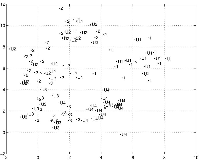
Figure 1: Example involving partially labeled data and an unknown class. Labeled are denonted by a single class number while unlabeled data are denoted by a ‘U’ followed by the class. The $x$s denote mixture component centers.

The 2-D data points were generated according to a Gaussian mixture with 5 components. For this example, all points originating from the same component come from the same class, i.e. classes “own” either one or multiple mixture components. In this example, class two consists of two components, with the other classes consisting of single components. Note that for the known classes, it appears in Fig. 1 (and is the case) that labels are missing at random, while for the unknown classes (class 4 in this case), labels are deterministically (always) missing. This is consistent with an expert labeler who randomly selects a subset of data from the known classes and is unable to label any data from unknown classes. In Miller & Browning (2003a) and Miller & Browning (2003b), mixture models were proposed that were tailored to this data scenario. In this work, we have applied the approach in Miller & Browning (2003b), summarized next.

Notation

Let ${\cal M}_{k}$, $k=1,\ldots,M$ denote the $k$th mixture component. Let ${\cal C}_{\rm pre}$ denote the subset of “predefined” components, with the remaining subset denoted ${\bar{\cal C}}_{\rm pre}$. Let $C\in{\cal P}_{c}\equiv\{1,2,\ldots,N_{c}\}$ be a random variable defined over the $N_{c}$ known classes, with $c(\underline{x})\in{\cal P}_{c}$ the class label paired with $\underline{x}$. Let $\alpha_{k}$ denote the prior probability for component $k$, $\theta_{k}$ the parameter set specifying component $k$’s (component-conditional) joint feature density, and let $P[\underline{x}|\theta_{k}]$ denote this density. We also introduce a new class set $\tilde{\cal P}_{c}=\{1,2,\ldots,N_{c},u\}$, consisting of the set ${\cal P}_{c}$ plus a value $u$, used to indicate that a sample is unlabeled. With respect to the class set $\tilde{\cal P}_{c}$, every sample is now labeled, with the unlabeled samples taking on the label values ‘u’. We suppose a different random label generator, conditioned on each mixture component, i.e. ${\rm Prob}[c|{\cal M}_{k}]\equiv\beta_{c|k},c\in\tilde{\cal P}_{c}$, where $\sum\limits_{c\in\tilde{\cal P}_{c}}\beta_{c|k}=1$. In summary, the model is based on the parameter set $\Lambda=\{\{\alpha_{k}\},\{\theta_{k}\},\{\beta_{c|k}\}\}$.

Hypothesis for Random Generation of the Data

This model Miller & Browning (2003b) hypothesizes that each sample from ${\cal X}_{m}$ is generated independently, based on $\Lambda$, according to the following stochastic generation process:

i) Randomly select a component ${\cal M}_{j}$ according to $\{\alpha_{k}\}$.

ii) Randomly select a vector $\underline{x}$ according to $P(\underline{x}|\theta_{j})$ and a label $c$ according to $\{\beta_{k|j}\}$.

Joint Data Likelihood

The log of the joint data likelihood associated with this model is

$${\cal L}=\sum\limits_{\underline{x}\in{\cal X}_{m}}\log\sum\limits_{k=1}^{M}\alpha_{k}f(\underline{x}|\theta_{k})\beta_{c(\underline{x})|k},$$ (1)

where $c(\underline{x})\in\tilde{\cal P}_{c}$. The model parameters $\Lambda$ can be chosen to maximize the log-likelihood (1) via the Expectation-Maximization (EM) algorithm (e.g. Duda, Hart, & Stork (2001)). Since the derivation of these EM equations is standard, their exposition is herein omitted.

This model does not explicitly discover new class components, i.e. mixture components that are purely unlabeled. However, suppose that, for a given component ${\cal M}_{j}$, we have that $\beta_{u|j}\simeq 1$ and $\beta_{u|j}$ is also significantly greater than the average value $\frac{1}{M}\sum\limits_{j^{\prime}=1}^{M}\beta_{u|j^{\prime}}$. In this case, the fraction of unlabeled data owned by the component is unusually high. We categorize these components as “nonpredefined”, i.e. ${\cal M}_{j}\in{\bar{\cal C}}_{\rm pre}$. Such components are putative unknown class components. All other components are categorized as “predefined”, representing known class data. To summarize, we have the following strategy for class discovery/outlier detection in mixed data: 1) learn a mixture model to maximize the log likelihood (1); 2) for each component, declare it “nonpredefined” if $\beta_{u|j}-(\frac{1}{M}\sum\limits_{j^{\prime}=1}^{M}\beta_{u|j^{\prime}})>\delta$; otherwise, declare it “predefined”. Here, $\delta$ is a suitably chosen threshold. In practice, we declare a component “nonpredefined” when its value $\beta_{u|j}$ is closer to $1.0$ than to the average value, i.e., we choose $\delta=\frac{1}{2}(1-\frac{1}{M}\sum\limits_{j^{\prime}=1}^{M}\beta_{u|j^{\prime}})$. We have found this choice for $\delta$ to give reasonable results for a variety of experimental conditions (for different data sets and for different fractions of labeled data).

Statistical Inferences from the Model

After applying this thresholding operation to each component, the resulting model is naturally applied to address several inference tasks: 1) standard classification of a given sample to one of the known classes; and 2) known vs. unknown class discrimination. For classification to known classes, for a given sample $\underline{x}$, we compute the a posteriori probabilities

$$P[C=c|\underline{x};\Lambda]=\frac{\sum\limits_{k\in{\cal C}_{\rm pre}}\alpha_{k}f(\underline{x}|\theta_{k})(\frac{\beta_{c|k}}{1-\beta_{u|k}})}{\sum\limits_{k\in{\cal C}_{\rm pre}}\alpha_{k}f(\underline{x}|\theta_{k})},c\in{\cal P}_{c}.$$ (2)

These can be used in a maximum a posteriori (MAP) class decision rule.

In order to discriminate between the hypotheses that an unlabeled sample originates from a known versus an unknown class, we need the a posteriori probability that the given feature vector is generated by a nonpredefined component. This is given by

$$P[{\cal M}_{\rm np}|\underline{x}\in{\cal X}_{u}]=\frac{\sum\limits_{k\in{\bar{\cal C}}_{\rm pre}}\alpha_{k}f(\underline{x}|\theta_{k})\beta_{u|k}}{\sum\limits_{k}\alpha_{k}f(\underline{x}|\theta_{k})\beta_{u|k}}$$ (3)

New Class Discovery

While the EM learning assumes that the number of mixture components $M$ is fixed and known, in practice this size must be estimated. Model order selection is a difficult and pervasive problem, with several criteria proposed (Schwarz, 1978; Wallace & Freeman, 1987; Mclachlan & Peel, 2000) and no consensus on the right one. In our class discovery setting, the importance of accurate model order selection cannot be overstated – the nonpredefined components in the validated solution will be taken as candidates for new classes, to be forwarded to a domain expert for further study. Accurate model order selection is thus important for successful new class discovery. Here, as in Miller & Browning (2003a), Miller & Browning (2003b) the Bayesian Information Criterion (BIC) (Schwarz, 1978) is applied. The BIC model selection criterion is written in the form

$$BIC(M)=\frac{N_{p}(M)}{2}\log N-{\cal L},$$ (4)

with $N_{p}(M)$ the number of free parameters in the $M$-component model and $N$ the data length. The first term is the penalty on model complexity, with the second term the negative log-likelihood. We applied BIC in a “wrapper-based” model selection approach; i.e., we built models for increasing $M$, evaluated each in terms of BIC, and selected the model with minimum cost.

While any clustering/mixture modeling technique can in principle be used to discover unknown classes, standard methods do not have any special impetus for finding label-free (or largely label-free) clusters. By contrast, the log likelihood (1) and the likelihood function used in Miller & Browning (2003a) both encourage solutions with nonpredefined components, when such components are warranted by the presence of unknown classes in the data. In (1), it is the $\beta_{c|j}$ term which provides the impetus for forming these unknown classes, since this term approaches its maximum value ($\beta_{u|j}=1$) in the nonpredefined component case.

3.2 Neural Network Approach

The mixture modeling approach provides several inference capabilities when dealing with mixed labeled/unlabeled data sets and possibly unknown classes: 1) it allows one to infer whether or not a given sample belongs to one of the known classes; 2) it identifies purely unlabeled mixture components/clusters, which are reasonably treated as putative unknown classes or, at any rate, components of unknown classes; 3) conditioned on a known class hypothesis for a given sample, the model can infer from which known class the sample originates (i.e., the usual classification inference capability).

While the mixture modeling approach is naturally suited to new class discovery given mixed labeled/unlabeled data, neural network (NN) classifiers do not appear to be predisposed to making these inferences. Neural networks are generally trained using a purely supervised approach, with class labels provided for every example in the training set. Thus, in general, unlabeled samples play no role in the training – given a mixed labeled/unlabeled data set, the NN training will discard all the examples from unknown classes, or, perhaps worse, erroneously impute and use known class labels for this unknown class data. Accordingly, the neural network is only explicitly trained to discriminate between the known classes – it is not trained to distinguish known from unknown classes. While it thus appears that neural networks do not possess any class discovery inference capability, we next suggest an approach that give NNs at least a weak form of this capability.

The neural network algorithm we used is a basic backpropagation algorithm available with the WEKA machine learning package Witten & Frank, (2000). We used the default configuration consisting of a three layer network (input, hidden, and output). The number of input nodes was $N_{i}$, one node for each input feature. There were $N_{c}$ output nodes, one for each known class. The number of hidden nodes was calculated according to $N_{h}=(N_{i}+N_{c})/2$. For the ESOLV data we used 12 nodes in the input layer corresponding to the 12 input features, eight nodes in the hidden layer, and four in the output layer. For the SDSS data we used five input layer nodes, five hidden layer nodes, and six output layer nodes.

Decision Confidence

Suppose the neural network produces (soft) discriminant function outputs $g_{j}(\underline{x})$ for each of the known classes $j=1,\ldots,N_{c}$. Let $\tilde{g}_{j}(\underline{x})=\frac{g_{j}(\underline{x})-\min_{l}g_{l}(\underline{x})}{\sum\limits_{k}g_{k}(\underline{x})-\min_{l}g_{l}(\underline{x})}$. With this choice, we have $0\leq\tilde{g}_{j}(\underline{x})\leq 1$ and $\sum\limits_{j}\tilde{g}_{j}(\underline{x})=1$, i.e. $\tilde{g}_{j}(\underline{x})$ is a probability mass function defined on the known classes. One principled measure of uncertainty in these soft decisions is the Shannon entropy $H=-\sum\limits_{j}\tilde{g}_{j}(\underline{x})\log\tilde{g}_{j}(\underline{x})$. If $H$ is greater than a preset threshold, we can declare that the sample $\underline{x}$ does not convincingly belong to any of the known classes, i.e. it is declared an unknown class sample. This approach, based on a measure of the classifier’s degree of indecision, is the one we have taken in imparting the neural network with some class discovery inference capability. Other measures of the classifier’s degree of indecision are also possible.

3.3 Error Measures

There are three error measures which we have used to evaluate the class discovery approaches. They are defined as follows:

Criterion 1: Misclassification rate in deciding between “known” and “unknown” class hypotheses.

This criterion was evaluated for both the mixture model and neural network approaches. For the mixture model, the classification decisions were made using a maximum a posteriori probability rule, based on (3). For the neural network, the decisions were made based on thresholding of the neural network’s entropy measure, as discussed earlier. The error rate was measured over the unlabeled portion of the data set (which consisted of both known and unknown class data), i.e. it was estimated as the fraction of unlabeled samples that were misclassified.

Criterion 2: Misclassification rate within “putative” unknown classes

The first criterion simply measures how effective an algorithm is at identifying the subset of (unlabeled) samples that come from new, i.e. unknown classes. If there is a single unknown class present in the data, then this is all that is required. However, suppose that there are multiple unknown classes present. Then, in addition to identifying the subset of samples from unknown classes, one would also like to identify the the individual classes which comprise this unknown class subset. In other words, one would like to identify the underlying cluster (group) structure within the unknown class data. The mixture modeling approach directly models the unknown and, separately, the known class data by a mixture of components (clusters). Each such cluster can be viewed as a putative unknown class. A measure of the accuracy of this clustering is the unknown class label purity of these clusters. In particular, suppose one of the learned nonpredefined clusters owns (in a MAP sense) 20 samples that are ground-truth from unknown class A, 30 samples from unknown class B, and 35 unlabeled samples that in fact belong to known classes. The most populous unknown class in the cluster is B. All samples in the cluster that do not possess label B are reasonably counted as errors. One can sum these errors over all nonpredefined clusters and divide by the total number of samples owned by all nonpredefined clusters. This is the fraction of samples that in effect have been erroneously assigned to individual nonpredefined clusters. Note that this criterion is only well-defined when the model finds at least one non-predefined component.

Criterion 3: Known class error rate

If a sample belongs to a known class, then we certainly will be interested in identifying to which known class it belongs. Accordingly, we can define an error fraction measured over the known class data. Several such criteria are possible. Here, we counted an error if an unlabeled sample that is from a known class is assigned to the wrong known class. For the mixture model, a MAP classification rule based on the probabilities (2) was used.

All three of the above criteria require various forms of ground truth label information for the unlabeled data subset – Criterion 1 requires a ground truth known/unknown class indication for all the data, Criterion 2 requires knowledge of unknown class labels for all the data, and Criterion 3 requires knowledge of all known class labels. Since in practice one would not have this information (by definition, no labels are known for data from unknown classes), these criteria can only be used for model evaluation/validation. In practice, other information sources or expert knowledge would be needed in order to assess the quality of, or to confirm, the model inferences. We also note that the second criterion can only be evaluated for the mixture model, since the neural network approach does not attempt to partition the estimated unknown class data into smaller groups.

4 Results

We evaluated the mixture model and neural network on both the ESOLV and SDSS data sets. For SDSS, we constrained mixture component variances to be at least 0.1 in order to avoid an observed tendency for the learning to find singular solutions (zero variance), as well as solutions with very small variances along some dimensions. For both the mixture model and the neural network there are “operating parameters” whose choices affect the class discovery inference performance. For the mixture model, we need to select the model order, i.e. the number of components. This choice will clearly affect the ability to identify unknown class components. For example, if an unknown class has a small mass, one or more components will only be “deployed” for its representation if the model has many components. Likewise, if the unknown class has a very large mass (and significant within-class variation), quite a few components may be needed to represent it well. For the neural network, the choice of the entropy threshold affects performance. We have performed several experimental evaluations of the mixture model and neural network, based on different approaches for choosing these operating parameters. In one set of experiments, shown for the ESOLV and SDSS data sets in Tables 3 and 4, we picked both the mixture order (over the range 10 to 80) and the NN’s entropy threshold (by an exhaustive search) to maximize Criterion 1 performance. Note that these approaches cannot be used in practice since, in performing the model selection, these methods require evaluating a cost (Criterion 1) that depends on knowledge of the unknown class labels. However, this experiment does allow a comparison of best-case performances achieved by the mixture and neural network approaches. For the mixture model, we have also applied BIC-based selection as described earlier. This approach is wholly unsupervised, and thus feasible in practice.

Tables 3 and 4 show the results for the ESOLV data and the SDSS data using the best (lowest) value for Criterion 1. The first column shows the classes that were treated as unknown for that series of runs. The value of “ncomp” is the number of components used by the mixture model corresponding to the best value of Criterion 1, while “nonpre” is the number of nonpredefined components used by that model. The remaining columns under “Mixture Model” list error fractions for the three criteria discussed above. Under “Neural Network” we list the value of Criterion 1, the only error measure evaluated for the neural network. The last column shows the percentage change in the Criterion 1 value between the neural network and the mixture model, with a negative value indicating a lower Criterion 1 error for the mixture model compared to the neural network. The bracketed values at the bottom of each column are the average values (across all experiments) over that column. For the moment we will restrict discussion to the Criterion 1 performance. Tables 3 and 4 show that, with both methods optimized for Criterion 1 performance, significantly better inference accuracy is achieved by the mixture-based approach. For the ESOLV data we find an average decrease in Criterion 1 error of $20\%$ and a maximum decrease of $50\%$. For the SDSS data we find an average decrease in Criterion 1 error of $57\%$ and a maximum decrease of $96\%$. This is not especially surprising, since the mixture is learned using the unknown class data (but without use of the labels), while the neural network is only trained on labeled known class data.

In Tables 5 and 6, we compare the neural network, again with the threshold optimized for Criterion 1, against the mixture model, but with the order now selected based on the BIC criterion. Since the neural network decision making threshold is optimized based on knowledge of the unknown class labels while the mixture model and its order are chosen without use of this information, this comparison is not a fair one. However, in practice unsupervised order selection will be required. Thus, this comparison does give insight into the loss in accuracy attributable to the use of, generally suboptimal, but practically feasible model order selection techniques. As Tables 5 and 6 show, the Criterion 1 error for the mixture model is now higher in 5 of 9 cases for the ESOLV data and is the same or higher in 5 of 13 cases for the SDSS data. For the ESOLV data we find an average $10\%$ increase in error, while for the SDSS data we find an average $20\%$ decrease in error, compared to the neural network.

Figure 2 shows a plot of the number of components in the best performing mixture model as a function of the fraction of objects in the unknown classes, for the ESOLV data. There is a clear trend toward a larger number of components needed to describe data sets where the unknown classes make up a larger mass fraction of the total data set. One point, with classes 0 and 2 as the unknown classes, is well described by an unexpectedly small number of components (13). This is discussed below. A similar trend is not evident in the SDSS data. The SDSS data are dominated by two classes (1 and 2) which together represent over 88% of the data.

Figure 2: Number of components in the best mixture model, using Criterion 1 model selection, as a function of class mass for ESOLV data. Points are labled by unknown class.

Figures 3 and 4 show plots of the value of the Criterion 1 error as a function of the number of components in the mixture model for two different unknown class combinations. These plots reflect the information in Figure 2 in a different way. When the unknown classes represent a relatively small mass fraction of the total number of objects in the data set, the minimum value of Criterion 1 is found at a relatively moderate number of components. For example, this is evident in the figure for unknown class 4. Conversely, as seen in Figure 2, if the unknown classes comprise a large fraction of the total number of objects in the data set, then a larger number of components is needed to explain the data and the minimum value of Criterion 1 is found at a correspondingly higher number of components. Note that in Figure 4 Criterion 1 remains static over a range of model orders (for unknown class 0, over the range 10-20 components). This is due to the fact that the performance only changes at discrete points, where additional nonpredefined components are introduced. In this case, no nonpredefined components were introduced until $M$ increased beyond 20.

Figure 3: Criterion 1 error as a function of the number of components in the mixture model using ESOLV data with unknown class 4.

Figure 4: Criterion 1 error as a function of the number of components in the mixture model using ESOLV data with unknown class 0.

Figures 5 and 6 show the Criterion 1 error as a function of the number of mixture model components for the SDSS data. Again we see the Criterion 1 error remaining pretty much static until the model order $M$ reaches 25 to 35 components. At this point nonpredefined components are added to the model allowing further decrease in the Criterion 1 error.

Figure 5: Criterion 1 error as a function of the number of components in the mixture model using SDSS data with unknown class 1.

Figure 6: Criterion 1 error as a function of the number of components in the mixture model using SDSS data with unknown classes 0 and 3.

The SDSS data contains approximately ten times the number of data points as the ESOLV data. The mixture model approach generally requires a larger number of components to describe the SDSS data set. On average 34 components were required to describe the ESOLV data using the best model by Criterion 1, while 61 components were needed to describe the SDSS data. Using BIC to determine the best model required on average 61 components for the ESOLV data and 71 for the SDSS data.

Table 3: Mixture model and neural network results using Criterion 1 error model selection for ESOLV data.

	Mixture Model						Neural Network
Unknown Class	ncomp	nonpre	Criterion 1	Criterion 2	Criterion 3		Criterion 1	$\Delta\%$
0	27	1	0.08859	0.7275	0.3742		0.09923	-10.7
1	42	1	0.1717	0.9036	0.3220		0.1810	-5.1
2	70	16	0.3797	0.5510	0.3083		0.4883	-22.2
3	48	5	0.2183	0.7482	0.3249		0.2408	-9.3
4	14	1	0.05110	0.5178	0.4221		0.07773	-34.3
0 1	16	4	0.1399	0.5588	0.3276		0.2805	-50.3
0 2	13	3	0.4553	0.6466	0.2140		0.6109	-25.5
0 3	39	4	0.3179	0.8479	0.2524		0.3403	-6.6
0 4	34	2	0.1463	0.7702	0.3573		0.1770	-17.3
	$<33.7>$	$<4.1>$	$<0.2188>$	$<0.6978>$	$<0.3230>$		$<0.2773>$	$<-20.2>$

Table 4: Mixture model and neural network results using Criterion 1 error model selection for SDSS data.

	Mixture Model						Neural Network
Unknown Class	ncomp	nonpre	Criterion 1	Criterion 2	Criterion 3		Criterion 1	$\Delta\%$
0	49	0	0.004711	NA	0.06145		0.004711	0
1	47	5	0.03319	0.2091	0.04596		0.1244	-73.3
2	28	20	0.03377	0.006797	0.1117		0.1344	-74.9
3	69	4	0.02181	0.1703	0.007064		0.09071	-76.0
4	47	0	0.004876	NA	0.06421		0.004876	0
5	68	0	0.002675	NA	0.06290		0.002675	0
6	74	1	0.01187	0.3382	0.08020		0.02105	-43.6
0 1	79	5	0.04074	0.2434	0.03501		0.1292	-68.5
0 2	33	20	0.03393	0.01153	0.09026		0.8673	-96.1
0 3	80	5	0.02483	0.2059	0.06232		0.09542	-73.9
0 4	66	1	0.009176	NA	0.07416		0.009587	-4.3
0 5	77	1	0.005719	0.6518	0.09580		0.007386	-22.6
0 6	76	1	0.01559	0.4553	0.06439		0.02576	-39.5
	$<61>$	$<4.8>$	$<0.01868>$	$<0.2547>$	$<0.06580>$		$<0.1167>$	$<-57.3>$

Table 5: Mixture model selected by BIC and neural network results on the ESOLV data.

	Mixture Model						Neural Network
Unknown Class	ncomp	nonpre	Criterion 1	Criterion 2	Criterion 3		Criterion 1	$\Delta\%$
0	60	7	0.1530	0.9206	0.3991		0.09923	54.2
1	53	10	0.2619	0.8672	0.3345		0.1810	44.7
2	63	11	0.4327	0.7428	0.3149		0.4883	-11.4
3	54	6	0.2564	0.8896	0.3067		0.2408	6.5
4	67	7	0.1033	0.6137	0.4373		0.07773	32.9
0 1	69	13	0.1902	0.6203	0.3184		0.2805	-32.2
0 2	57	8	0.5253	0.7985	0.2091		0.6109	-14.0
0 3	62	11	0.3394	0.8542	0.2369		0.3403	-0.3
0 4	62	7	0.2004	0.7726	0.3684		0.1770	13.2
	$<60.8>$	$<8.9>$	$<0.2736>$	$<0.7866>$	$<0.3250>$		$<0.2773>$	$<10.4>$

Table 6: Mixture model selected by BIC and neural network results on the SDSS data.

	Mixture Model						Neural Network
Unknown Class	ncomp	nonpre	Criterion 1	Criterion 2	Criterion 3		Criterion 1	$\Delta\%$
0	70	0	0.004711	NA	0.1100		0.004711	0
1	63	5	0.1044	0.5353	0.03800		0.1244	-16.1
2	67	24	0.09999	0.03841	0.09737		0.1344	-25.7
3	74	5	0.02273	0.06070	0.1053		0.09071	-74.9
4	76	0	0.004876	NA	0.1060		0.004876	0
5	80	1	0.002921	0.5389	0.1178		0.002675	9.2
6	71	3	0.02732	0.6661	0.1066		0.02105	29.8
0 1	66	5	0.09434	0.4886	0.03388		0.1292	-27.0
0 2	79	30	0.1128	0.02745	0.06373		0.8673	-87.0
0 3	74	5	0.03306	0.1450	0.10390		0.09542	-65.4
0 4	61	1	0.009505	0.5297	0.1121		0.009587	-0.9
0 5	71	1	0.006275	0.6044	0.1116		0.007386	-15.0
0 6	71	3	0.02732	0.6661	0.1066		0.02576	6.1
	$<71>$	$<6.4>$	$<0.04233>$	$<0.3910>$	$<0.09330>$		$<0.1167>$	$<-20.5>$

5 Discussion

As can be seen from the results presented above we are, in general, able to achieve a significantly lower Criterion 1 error value when using unlabeled data to augment the labeled data. Overall, we obtained a $22\%$ (listed in table 3 as the fraction $0.2188$ not as the percent) Criterion 1 error for ESOLV data and a $2\%$ error for SDSS data when using Criterion 1 as the model selection method. When using BIC for model selection we obtained $27\%$ error for ESOLV data and $4\%$ error for SDSS data. The percentage change column of Table 3 shows that on average the mixture models reduced the Criterion 1 error for ESOLV data by $20\%$, but this reduction was as high as $50\%$ when classes 0 and 1 were unknown. Table 4 similarly shows an average $57\%$ reduction in Criterion 1 error for SDSS data with a $96\%$ reduction when classes 0 and 2 were unknown. A $20\%$ reduction in error for the ESOLV data implies an extra 1043 out of 5217 objects were correctly classified by the mixture model compared to the neural network. For the SDSS data a $57\%$ error reduction implies an additional 30784 out of 54007 objects were correctly classified by the mixture model.

Our study is the first to apply semisupervised learning to astronomical data, and the first, to our knowledge, to use a data set as large as 50000 points. This is an important test of the methodology because of the vast amount of astronomical data freely available today, most of which is unlabeled. Demonstrating that our methods work with large astronomical data sets was a primary goal of this work.

Nevertheless, there are a number of factors that influence the reliability of the proposed method and what level of error can be achieved. The results in Tables 3-6 demonstrate the importance of the model order selection technique. BIC-based selection fares well on the SDSS data, achieving substantially better average Criterion 1 results than the neural network optimized for Criterion 1 and only modestly worse results than the mixture model optimized for Criterion 1 (0.02 vs. 0.04 average error rates). However, there is a significant average performance gap between the two mixture approaches on the ESOLV data (0.22 vs. 0.27) and the BIC-selected mixture is only comparable to the neural network on ESOLV (0.273 vs. 0.277 average error rates). It is possible that a better model order selection technique could improve the mixture results on ESOLV.

One artifact of optimizing the mixture for Criterion 1 is that, on average, smaller models are selected, compared with the mixtures selected by BIC. For ESOLV on average 34 components were selected by the former approach, while on average 61 components were selected by the latter. Furthermore, an average of 4.1 nonpredefined components were used with Criterion 1 model selection while an average of 8.9 were used with BIC. For the SDSS data an average of 61 components, including 4.8 nonpredefined components, were selected using Criterion 1. Finding the best SDSS model by BIC we needed on average 71 components, including 6.4 nonpredefined components. While we learned models with up to 80 components, in some cases for the SDSS data the best models were using close to 80 components. This suggests it may be reasonable to evaluate solutions with even more components. While the mean number of components selected by BIC was greater than that selected according to Criterion 1, the variance in the number of selected components is much greater for selection according to Criterion 1. This is consistent with the results in Figure 2, which indicate that, for best Criterion 1 performance, the number of components is significantly correlated with the mass of the unknown classes (which varies greatly since the classes are far from equally likely). This further means that, in some cases, when the mass of the unknown classes is large, Criterion 1 selects more components than BIC. For example, for the ESOLV data, class 2 occurs $46\%$ of the time. When this class is taken as unknown, BIC selected 63 components, while Criterion 1 selected 70.

Another factor that influences model accuracy is the fact that the learning objective function ${\cal L}$ is multimodal, with significant potential for finding suboptimal local maxima, rather than the global maximum. At each model order, we generated several solutions based on different initializations and picked the one with greatest log-likelihood. However, there is anecdotal evidence in our results that we may only be finding locally optimal solutions at each model order. Referring back to Figure 2 we see that the best model for unknown classes 0 2 contains only 13 mixture components. This clearly is not in keeping with the trend that more mixture components are needed to explain the data with larger mass fraction of unknown classes. It appears in this case that a particularly good solution was found. This likewise suggests that, at other orders, suboptimal, local maximum solutions were found.

The Criterion 2 error is a measure of how well the algorithm can classify objects within the newly found classes. This is a very hard problem because we are asking the algorithm to do two things. First, determine if some mixture components (the nonpredefined components) are needed to describe objects that do not fit into the existing known class structure. Second, partition these objects correctly between the unknown class components. This second step is effectively looking for substructure in the newly discovered classes.

For the ESOLV data we found on average about a $70\%$ Criterion 2 error compared with about a $25\%$ error for the SDSS data when using Criterion 1 model selection. Similarly, we find about $79\%$ error for the ESOLV data and $39\%$ error for SDSS data when using BIC model selection. The values of NA for Criterion 2 error for some of the SDSS experiments reflect models where there were no nonpredefined components; in this case the error measure is undefined. Note that, in all these cases, the unknown classes had very small mass, which explains why no nonpredefined components were found. In particular, class 0 and class 4 collectively comprise less than $1\%$ of the SDSS data. Thus, when these classes are missing, we would not expect to find nonpredefined components in the solution unless both 1) there are more than 100 components in the model and 2) the model criterion selects a solution of this size.

The Criterion 3 error measures how well the model can assign objects to known classes. For this we obtained about a $32\%$ error for ESOLV data and $7\%$ error for SDSS data using Criterion 1 model selection. When using BIC model selection we obtained $33\%$ error for ESOLV data and $9\%$ error for SDSS data.

We find the overall results presented here very promising. The tests done here have demonstrated the efficacy of the class discovery problem and approaches. However, more work will be required to develop a mature technology for highly reliable new class discovery.

6 Acknowledgments

We would like to thank the NASA Applied Information Systems Research Program for supporting us in this effort under contract NAS5-02098. One of the authors (DB) would like to thank Ofer Lahav for supplying the ESO-LV data.

References

- Banfield & Raftery (1993) Banfield J. D., & Raftery, A. E. 1993, Biometrics, 39, 803
- Basu et al. (2002) Basu, S., Banerjee, A. & Mooney, R. 2002, Intl. Conf. on Machine Learning, 1, 19
- Bazell & Aha (2001) Bazell, D. & Aha, D. W. 2001, ApJ, 548, 219
- Duda, Hart, & Stork (2001) Duda, R. O., Hart, P. E., & Stork, D. G. 2000, Pattern Classification (2nd ed.; New York: Wiley)
- Lauberts & Valentijn (1989) Lauberts A. & Valentijn E. A. 1989, The Surface Photometry Catalogue of the ESO-Uppsala Galaxies, ESO
- Mclachlan & Peel (2000) McLachlan, G. & Peel, D. 2000, Finite Mixture Models, (New York: Wiley)
- Miller & Browning (2003a) Miller D. J. & Browning, J. 2003, IEEE Trans. on Pattern Anal. and Machine Intell., 25, 1468
- Miller & Browning (2003b) Miller D. J.,& Browning, J. 2003, IEEE Intl. Workshop on Neural Networks for Signal Processing, Toulouse, France, 1, 489
- Miller & Uyar (1997) Miller D. J., & Uyar, H. 1997, Neural Information Processing Systems, 9, 571
- Nigam et al. (2000) Nigam K., McCallum, A., Thrun, S., & Mitchell, T., 2000, Machine Learning, 39, 1
- Owens et al. (1996) Owens E. A. Griffiths, R. E., & Ratnatunga, K. U. 1996, MNRAS, 281, 153.
- Schwarz (1978) Schwarz G. 1978, Annals of Statistics, 6, 461
- Shashahani & Landgrebe (1994) Shashahani B., & Landgrebe D. 1994, IEEE Trans. on Geo. and Remote Sens., 32, 1087