BBN For Pedestrians

Abstract

The simplest, “standard” model of Big Bang Nucleosynthesis (SBBN) assumes three light neutrinos (N_ν = 3) and no significant electron neutrino asymmetry ($\nu_{e}-\bar{\nu}_{e}$ asymmetry parameter $\xi_{e}\equiv\mu_{e}/kT$, where $\mu_{e}$ is the $\nu_{e}$ chemical potential) leaving only one adjustable parameter: the baryon to photon ratio $\eta\equiv n_{\rm B}/n_{\gamma}$. The primordial abundance of any one nuclide can, therefore, be used to measure $\eta$ and the value derived from the observationally inferred primordial abundance of deuterium closely matches that from current non-BBN data, primarily from the WMAP survey. However, using this same estimate, there is a tension between the SBBN-predicted helium-4 and lithium-7 abundances and their current, observationally inferred primordial abundances, suggesting that N_ν may differ from the standard model value of three and/or that $\xi_{e}$ may differ from zero (or, that systematic errors in the abundance determinations have been underestimated or overlooked). The differences are not large and the allowed ranges of the BBN parameters ($\eta$, $N_{\nu}$, and $\xi_{e}$) permitted by the data are quite small. Within these ranges, the BBN-predicted abundances of D, ³He, ⁴He, and ⁷Li are very smooth, monotonic functions of $\eta_{10}$, $\Delta N_{\nu}\;$$\equiv$ N${}_{\nu}-3$, and $\xi_{e}$. As a result, it is possible to describe the dependencies of these abundances (or powers of them) upon the three parameters by simple, linear fits which, over their ranges of applicability, are accurate to a few percent or even better. The fits presented here have not been maximized for their accuracy but, rather, for their simplicity. To identify the ranges of applicability and relative accuracies, they are compared to detailed BBN calculations; their utility is illustrated with several examples. Given the tension within BBN, these fits should prove useful in facilitating studies of the viability of various options for non-standard physics and cosmology, prior to undertaking detailed BBN calculations.

I  Big Bang Nucleosynthesis

Shortly after the emergence of the Big Bang model it was realized that conditions were ripe during the early Universe for a brief period of nucleosynthesis. Just as in every other setting where nuclear reactions occur, the yields of the emerging nuclides are governed by three environmental characteristics: the duration of the event, the density of the reactants, and their thermal properties. A brief, dilute and cool environment would yield a very different set of abundances compared to those that would emerge if Big Bang Nucleosynthesis (BBN) had been long-lasting, dense and hot. Although it is possible to characterize BBN in such broad generality (with some success; see, for example, CK2002 ; MR2003 ), the paradigm most frequently encountered uses the Friedman equation to relate the BBN expansion rate, $H$, to the thermal properties of the particles present at that epoch

$$H^{2}=\frac{8\pi G_{N}}{3}\;\rho,$$ (1)

with $G_{N}$ being Newton’s constant and $\rho$ the total energy density. The standard model of particle physics provides the candidate particles whose energy density contribute to $\rho$, but it is possible that this may fall short of the actual particle content at that time. Even so, after blueshifting the currently observed Cosmic Background Radiation (CBR) energy density back to the epoch of BBN, it emerges that the energy density of the Universe was dominated during BBN by the relativistic particles. The thermal properties of each particle species are described by a temperature and a chemical potential, but thermal coupling among the constituents equilibrates the temperatures while chemical coupling relates the chemical potentials. Charge neutrality provides additional relations. This reduces the number of independent quantities with the result that BBN can be described by a minimal set of parameters, typically taken to be: the density of the nucleons/baryons, the chemical potentials of the three, active neutrinos, and the energy density in unaccounted particles (and/or additional terms on the right hand side of eq. 1). In what follows the role of each is discussed and the parameters used to describe them are introduced.

I.1  The Baryon Density: $\eta$

The simplest, “standard” model for BBN (SBBN) sets any “extra” energy density and the chemical potentials of the three neutrinos to zero leaving just the density of the baryons, $n_{\rm B}$, as the only adjustable/free parameter. But since $n_{\rm B}$ drops as the Universe expands, it is useful to introduce the baryon to photon ratio $\eta\equiv n_{\rm B}/n_{\gamma}$, ($\eta_{10}\equiv 10^{10}\eta$), since this quantity is dimensionless and constant, except during the period of $e^{\pm}\;$annihilation.

From inspection of the flow of nuclei through the reaction network in SBBN it can be seen that the primordial abundances of the relic light nuclides D, ³He, and ⁷Li are determined by the competition between the nuclear production and destruction rates, which scale with the nucleon density. To an extent which varies from nuclide to nuclide, these three nuclei are all potential baryometers. In contrast, as the light nucleus with the largest binding energy per nucleon, the ⁴He relic abundance is relatively insensitive to the magnitudes of the nuclear reaction rates because, for the range in baryon density of interest here, they are sufficiently rapid to burn nearly all neutrons present initially to ⁴He. What sensitivity it does possess is due to the role that $\eta$ plays in determining the temperature at which the D abundance becomes significant: it is the build up of a large D abundance that leads to the most rapid phase of nuclear burning in BBN and the termination of free neutron decay as an important process.

I.2 Early-Universe Expansion Rate: $S$

The early Universe is radiation-dominated, with its expansion rate determined by the energy density in the relativistic particles, $\rho_{\rm R}$. Prior to BBN, e.g., at a temperature of a few MeV, before $e^{\pm}\;$annihilation, the standard model of particle physics provides photons, $e^{\pm}\;$pairs and three flavors of left-handed (i.e., one helicity state) neutrinos (and their right-handed, antineutrinos) as constituents of this dominant component. With all chemical potentials set to zero the energy densities are related by thermal equilibrium so that

$$\rho_{\rm R}=\rho_{\gamma}+\rho_{e}+3\rho_{\nu}={43\over 8}\rho_{\gamma},$$ (2)

where $\rho_{\gamma}$ is the energy density in the CBR photons (which, today, have redshifted to become the cosmic background radiation photons observed at a temperature of 2.7K). In this case, the time-temperature relation (derived from the Friedman equation) is,

$${\rm Pre-e^{\pm}\;annihilation}:~{}~{}t~{}T_{\gamma}^{2}=0.738~{}{\rm MeV^{2}~{}s}.$$ (3)

In SBBN it is often assumed that the neutrinos are fully decoupled prior to $e^{\pm}\;$annihilation and that they don’t share in the energy transferred from the annihilating $e^{\pm}\;$pairs to the CBR photons. In this approximation, the photons are hotter than the neutrinos in the post-$e^{\pm}\;$annihilation universe by a factor $T_{\gamma}/T_{\nu}=(11/4)^{1/3}$, and the relativistic energy density is

$$\rho_{\rm R}=\rho_{\gamma}+3\rho_{\nu}=1.68\rho_{\gamma},$$ (4)

corresponding to a new time-temperature relation,

$${\rm Post-e^{\pm}\;annihilation}:~{}~{}t~{}T_{\gamma}^{2}=1.32~{}{\rm MeV^{2}~{}s}.$$ (5)

In quite general terms, one possible consequence of new physics beyond the standard model could be a non-standard, early Universe expansion rate, parameterized by an expansion rate factor $S$,

$$H\rightarrow H^{\prime}\equiv SH.$$ (6)

Although the introduction of $S$ here is quite general, in practice one must adopt a specific scheme through which this occurs. Such a non-standard expansion rate might, but need not, be due to a change in the energy density: a change in the strength of gravity would also alter the expansion rate of the early Universe KS2003 as would non-standard, higher dimensional models which modify the expansion rate – energy density relation (the Friedman equation, eq. 1) in our 3+1 dimensional world rs . Different gravitational couplings for fermions and bosons BS2004 would have similar effects. These different mechanisms for implementing a non-standard expansion rate are not necessarily equivalent.

If consideration is restricted to only the possibility of additional energy density, then

$$\rho_{\rm R}\rightarrow\rho_{\rm R}^{\prime}\equiv S^{2}\rho_{\rm R},$$ (7)

where $\rho_{\rm R}^{\prime}=\rho_{\rm R}+\rho_{X}$ and $X$ identifies the extra component. With the further restriction that the $X$ are also relativistic, this extra component behaves just like an additional neutrino though we emphasize that “X” need not be additional flavors of active or sterile neutrinos. In these circumstances S is a constant prior to $e^{\pm}\;$annihilation and it is convenient to account for the extra contribution to the standard-model energy density by normalizing it to that of an “equivalent” neutrino flavor ssg , so that

$$\rho_{X}\equiv\Delta N_{\nu}\rho_{\nu}={7\over 8}\Delta N_{\nu}\rho_{\gamma}.$$ (8)

For this case,

$$S\equiv S_{pre}=(1+{7\over 43}\Delta N_{\nu})^{1/2}.$$ (9)

However the expansion rate is more fundamental to BBN than is $\Delta N_{\nu}$, so we parameterize this class of non-standard models using $S$ (but, for comparison, we will often also quote the corresponding value of $\Delta N_{\nu}\;$as given by eq. 9).

Not every additional energy density component can be accommodated this way since we are requiring that $\rho_{X}$ is proportional to $\rho_{\nu}$ as the Universe evolves. An example that breaks this mold is if the “X” were not ‘decoupled’, in the sense that $X$ shared in the energy released when the $e^{\pm}\;$pairs annihilate. Other examples are found within some quintessence models SDTY1992 ; SDT1993 ; BHM2001 ; KS2003 .

As we discussed above, D, ³He, and ⁷Li act as the principle baryometers for BBN since the ⁴He relic abundance does not vary considerably with $\eta$. But ⁴He is very sensitive to the competition between the weak interaction rates (interconverting neutrons and protons) and the universal expansion rate which, during the early, radiation dominated evolution is fixed by the energy density in relativistic particles (“radiation”). As a result, while D, ³He, and ⁷Li probe the baryon density, consistency between their abundances and that of ⁴He tests the standard model and provides constraints on (and, perhaps, hints of) physics beyond the standard model.

I.3 Lepton Asymmetry: $\xi$

The baryon-to-photon ratio $\eta=n_{\rm B}/n_{\gamma}$ provides a dimensionless measure of the universal baryon asymmetry which is very small ($\eta~{}\lower 2.58334pt\vbox{\hbox{$\buildrel\textstyle<\over{\sim}\ $}}10^{-9}$). By charge neutrality the asymmetry in the charged leptons must also be of this order. However, there are no direct observational constraints (see ks92 ; kssw01 ; barger03b and further references therein), on the magnitude of any asymmetry among the neutral leptons (neutrinos). A dimensionless measure of the magnitude of the neutral lepton asymmetry is provided by $\xi$, the ratio of the neutral lepton chemical potential to the temperature (in energy units): $\xi\equiv\mu/kT$. For example, for a neutrino flavor $\alpha$, the asymmetry (“neutrino degeneracy”) $L_{\alpha}$, between the numbers of $\nu_{\alpha}$ and $\bar{\nu}_{\alpha}$ is

$$L_{\alpha}\equiv{n_{\nu_{\alpha}}-n_{\bar{\nu}_{\alpha}}\over n_{\gamma}}={\pi^{2}\over 12\zeta(3)}\bigg{(}\xi_{\alpha}+{\xi_{\alpha}^{3}\over\pi^{2}}\bigg{)}\,.$$ (10)

Note that for $\xi_{\alpha}\ll 1$, $L_{\alpha}\approx 0.684\xi_{\alpha}$. Mixing among the three active neutrinos ($\nu_{e},\nu_{\mu},\nu_{\tau}$) ensures that at the time of BBN, $L_{e}\approx L_{\mu}\approx L_{\tau}$ ($\xi_{e}\approx\xi_{\mu}\approx\xi_{\tau}$) equal .

While any neutrino degeneracy ($\xi_{\alpha}<0$ as well as $>0$) will increase the energy density in the relativistic neutrinos and, hence, the early Universe expansion rate, the discussion here is limited to sufficiently small values of $\xi_{\alpha}$ so that the effect on $S$ of a non-zero $\xi_{\alpha}$ is negligible. Even so, a non-zero but relatively small asymmetry between electron type neutrinos and antineutrinos ($\xi_{e}~{}\lower 2.58334pt\vbox{\hbox{$\buildrel\textstyle>\over{\sim}\ $}}10^{-2}$), while large compared to the baryon asymmetry, can still have a significant impact on the early Universe. The interconversion of neutrons to protons is affected by the $\nu_{e}$ so that any non-zero $\xi_{e}$ will alter the n/p ratio, thereby affecting the yields of the light nuclides formed during BBN.

Of the light nuclei, the neutron limited ⁴He abundance is the most sensitive to $\xi_{e}$ and, together with the D, ³He, and ⁷Li baryometers, again provides a test of the consistency of the standard model.

I.4 BBN Predictions

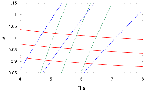
Figure 1: BBN-predicted isoabundance curves for D (dotted), ⁷Li (dashed), and ⁴He (solid) in the expansion-rate parameter ($S$), baryon density parameter ($\eta$) plane. From left to right, for D, $y_{\rm D}$ = 4, 3, 2, while for ⁷Li, $y_{\rm Li}$ = 3, 4, 5. For ⁴He, from bottom to top, Y_P = 0.23, 0.24, 0.25.

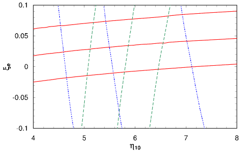
Figure 2: BBN-predicted isoabundance curves for D (dotted), ⁷Li (dashed), and ⁴He (solid) in the lepton asymmetry parameter ($\xi_{e}$), baryon density parameter ($\eta$) plane. From left to right, for D, $y_{\rm D}$ = 4, 3, 2, and for ⁷Li, $y_{\rm Li}$ = 3, 4, 5. For ⁴He, from top to bottom, Y_P = 0.23, 0.24, 0.25.

The BBN-predicted D, ⁴He, and ⁷Li isoabundance curves for $S$ versus $\eta$ and for $\xi_{e}$ versus $\eta$ are shown in Figures 1 and 2. For D, the curves represent the ratio (to hydrogen) by number $y_{\rm D}$ $\equiv 10^{5}$(D/H) = 2, 3, 4; similarly, for ⁷Li, the curves correspond to $y_{\rm Li}$ $\equiv 10^{10}$(Li/H) = 3, 4, 5; for ⁴He, the curves correspond to the mass fraction Y_P = 0.23, 0.24, 0.25. These figures show clearly that D and ⁷Li are good baryometers, sensitive to $\eta$, while ⁴He is a good chronometer, sensitive to $S$, as well as a good leptometer, sensitive to $\xi_{e}$.

II Observed Primordial Abundances

The success of Big Bang Nucleosynthesis relies on its ability to predict the observed primordial abundances and, conversely, to learn about the cosmological parameters using these same abundances. However the comparison of predictions and observations is far from trivial because of the further processing of the nuclei since the end of BBN.

Deuterium is the baryometer of choice, primarily because since BBN its observed abundance should have only decreased as gas is cycled through stars where D is burned to heavier, more tightly bound, nuclei els . As a result, D observed anywhere in the Universe, at any time during its evolution, should provide a lower bound to its primordial abundance. Further, the deuterium observed in the high redshift, low metallicity QSO absorption line systems (QSOALS) should be very nearly primordial. In contrast, the post-BBN evolution of ³He and of ⁷Li are considerably more complicated, involving the competition between production, destruction, and survival. As a result, at least so far, the current, locally observed (in the Galaxy) abundances of these nuclides have been of less value than has that of deuterium. Indeed, over the range in $y_{\rm D}$ to be adopted below, the primordial abundance of ³He is predicted to lie in the narrow range, $1.0~{}\lower 2.58334pt\vbox{\hbox{$\buildrel\textstyle<\over{\sim}\ $}}y_{3}~{}\lower 2.58334pt\vbox{\hbox{$\buildrel\textstyle<\over{\sim}\ $}}1.1$, in excellent agreement with that inferred from Galactic observations rood . Thus, ³He provides similar, but less compelling constraints than does D. While current estimates of primordial lithium, based on observations of very metal-poor (nearly primordial) stars, are problematic, ⁷Li is retained here in order to highlight this challenge. For ⁴He the post-BBN evolution is straightforward, but difficult to quantify at a sufficient level of accuracy. As gas is cycled through stars, hydrogen is burned to helium; only a very small fraction of the helium is burned to heavier nuclei. If material is sampled “here and now”, a correction based on models of the chemical evolution of galaxies would need to be made for post-BBN produced ⁴He. To avoid the model-dependent uncertainties associated with such corrections, which would surely overwhelm the observational errors, the best strategy is to search for ⁴He in the least evolved objects, in this case the metal-poor, extragalactic H $\scriptstyle{\rm II}$ regions.

Inferring the primordial D abundance from the QSOALS has not been without its difficulties, with some of the original abundance claims having been withdrawn or revised. Presently there are 5 – 6 QSOALS with reasonably firm deuterium detections bta ; btb ; o'm ; pb ; dod ; k . However, there is significant dispersion among the abundances and the data fail to reveal the anticipated “deuterium plateau” at low metallicity or at high redshift gs01 . Here we adopt the five abundance determinations collected in the recent paper of Kirkman et al. k . The weighted mean value of $y_{\rm D}$ is 2.6 . The dispersion among these five data points is very large, resulting in a $\chi^{2}=15.3$ for four degrees of freedom, suggesting that one or more of these abundance determinations may be in error, or affected by unidentified and unaccounted for systematic errors. To allow for this, we follow the approach advocated by o'm and k and adopt for the uncertainty in $y_{\rm D}$ the dispersion among the data points divided by the square root of the number of them. Thus, the primordial abundance of deuterium to be used here is chosen to be: $y_{\rm D}$ $=2.6\pm 0.4$.

A somewhat less than clear situation also exists for the determinations of the primordial abundance of ⁴He. There have been two, largely independent, estimates of Y_P based on analyses of large data sets of low-metallicity, extragalactic H $\scriptstyle{\rm II}$ regions. The “IT” itl ; it estimate of Y(IT) $=0.244\pm 0.002$, and the “OS” determination os ; oss ; fo of Y(OS) $=0.234\pm 0.003$ which differ by nearly $3\sigma$. Very recently, IT have expanded their original data set and attempted to account for some (but not all) of the systematic uncertainties it04 ; see, e.g.,  os04 . For their full data set of 89 H $\scriptstyle{\rm II}$ regions, IT find Y_P $=0.2429\pm 0.0009$. To provide a contrast with previous results, this value is adopted for our analysis here.

As with ⁴He, the abundance of ⁷Li grows in the course of post-BBN evolution, with lithium being produced in some stars (at some distinct times in their evolution) as well as in cosmic ray spallation reactions (where CNO nuclei are broken down to, among other nuclides, lithium). So, as for D and ⁴He, lithium should be observed in the least evolved, most metal-poor objects. While lithium has been observed in the Sun and in the solar system, as well as in the interstellar medium of the Galaxy, these provide evolved, metal-enriched samples of little use in estimating the primordial abundance of lithium. The most relevant data comes from studies of the very metal-poor stars in the halo of the Galaxy or in Globular Clusters. While this material should be very nearly primordial, it must be kept in mind that these are observations of the surfaces of the oldest stars in the Galaxy. If, during the course of their evolution, the surface material of these stars were mixed with the lithium-depleted interiors, the currently observed surface lithium abundances may not reflect the lithium abundances in these stars at their birth. The most recent data from studies of halo stars is from Ryan et al. ryan who find $y_{\rm Li}$ $=1.23^{+0.34}_{-0.16}$. In contrast, and in some conflict with this result, Bonifacio et al. bonif derive from a sample of Globular Cluster stars, $y_{\rm Li}$ $=2.19^{+0.46}_{-0.38}$.

Below we compare each of these estimates of the primordial abundances with the BBN predictions, standard as well as non-standard, fixed by the adopted D and ⁴He abundances.

III Fits

The non-linear, coupled differential equations of BBN are not conducive to analytic solution so that detailed comparison of the theoretical predictions with the observed/derived abundances of the light nuclei can only be achieved after resorting to a lengthy process of numerical calculations. This necessity blurs the connection between the parameter set {$\eta$, $S$, $\xi_{e}$} and the data set {$y_{\rm D}$, Y_P, $y_{\rm Li}$}, and, conversely, the parameter values the data recommend. Yet it is clear from Figures 1 and 2 that the relic light nuclide abundances are smoothly varying, monotonic functions of $\eta$, $S$, and $\xi_{e}$, so it isn’t surprising that over limited but substantial ranges, simple relations exist between the predicted abundances and these parameters. While the BBN-predicted primordial abundances are certainly not linearly related to the baryon density, the expansion rate, or the lepton asymmetry, our goal here is to find simple, linear fits to the predicted abundances (or powers of them) as functions of these parameters (to be defined more carefully below). These fits work well, sometimes remarkably well, over limited ranges in the parameters (and/or over limited ranges in the predicted abundances of D, ⁴He, and ⁷Li).

Since the domains over which our fits are applicable are restricted, we must focus upon specific values for $\eta$, $S$ and $\xi_{e}$. The “target” value/range of the baryon density is motivated by the (non-BBN) results from the WMAP constraints from the CBR temperature fluctuations sperg where, for SBBN, $\eta_{10}=6.14\pm 0.25$. As shown in barger03a ; barger03b (and references therein), this estimate is little affected by a non-standard expansion rate and/or any (small) lepton asymmetry. As a result, a limited range in $\eta_{10}$, centered around $\eta_{10}=6$, is chosen here: $4\leq\eta_{10}\leq 8$. For our simple, linear fits to the BBN-predicted abundances as a function of $S$ to be sufficiently accurate, we must restrict the range in $S$. This is the case for the fits we adopt provided that $0.85\leq S\leq 1.15$ corresponding to $-1.7~{}\lower 2.58334pt\vbox{\hbox{$\buildrel\textstyle<\over{\sim}\ $}}\Delta$N${}_{\nu}~{}\lower 2.58334pt\vbox{\hbox{$\buildrel\textstyle<\over{\sim}\ $}}2.0$ ($1.3~{}\lower 2.58334pt\vbox{\hbox{$\buildrel\textstyle<\over{\sim}\ $}}$N${}_{\nu}~{}\lower 2.58334pt\vbox{\hbox{$\buildrel\textstyle<\over{\sim}\ $}}5.0$). For an “interesting” range in $\xi_{e}$ over which the fits are reasonably accurate, $-0.1\leq\xi_{e}\leq 0.1$ is adopted.

Before presenting our fits, it is worth reemphasizing that Figures 1 & 2 show clearly that D and ⁷Li are good baryometers, sensitive to $\eta$, while ⁴He is a good chronometer, sensitive to $S$, as well as a good leptometer, sensitive to $\xi_{e}$.

III.1  Helium-4

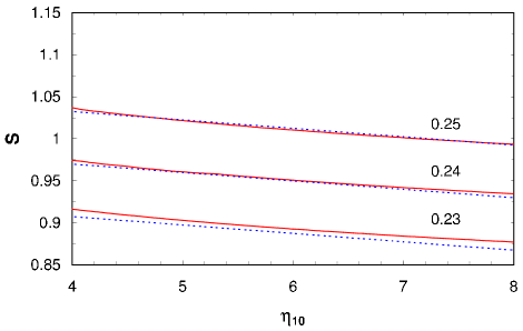
Figure 3: BBN-predicted isoabundance curves for ⁴He in the expansion-rate parameter ($S$), baryon density parameter ($\eta$) plane. From bottom to top, Y_P = 0.23, 0.24, 0.25. The solid curves are the BBN-predicted results, while the dotted curves are our fits (see the text).

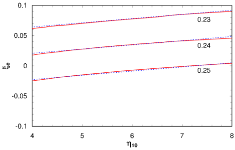
Figure 4: BBN-predicted isoabundance curves for ⁴He (solid) in the lepton asymmetry parameter ($\xi_{e}$), baryon density parameter ($\eta$) plane. From top to bottom, Y_P = 0.23, 0.24, 0.25. The solid curves are the BBN-predicted results, while the dotted curves are our fits (see the text).

The ⁴He abundance (mass fraction: Y_P) is very insensitive to the baryon density at BBN, varying roughly logarithmically with $\eta$ over the range of $\eta$ adopted here ($4~{}\lower 2.58334pt\vbox{\hbox{$\buildrel\textstyle<\over{\sim}\ $}}\eta_{10}~{}\lower 2.58334pt\vbox{\hbox{$\buildrel\textstyle<\over{\sim}\ $}}8$). Thus, while for SBBN ($S=1$ and $\xi_{e}$ = 0) to a very good approximation Y = Y($\eta)\propto~{}$ln $\eta$, we prefer to find a linear relation between Y_P and $\eta$. Motivated by simplicity, the following linear fit for Y versus $\eta$ agrees with the SBBN-predicted predicted abundance to within 0.0006 ($\lower 2.58334pt\vbox{\hbox{$\buildrel\textstyle<\over{\sim}\ $}}0.25\%$) over our adopted range in $\eta$.

$$Y_{\rm P}^{FIT}\equiv 0.2384+0.0016\eta_{10}=0.2384+\eta_{10}/625.$$ (11)

We note that over the same range in $\eta$ this fit also agrees with the BNT bnt predictions for Y_P to within 0.0002 ($\lower 2.58334pt\vbox{\hbox{$\buildrel\textstyle<\over{\sim}\ $}}0.1\%$) or better. While the accuracy of this fit is certainly not perfect, the difference is still smaller than the current errors in the observationally inferred primordial value of Y_P.

As with the Y_P – $\eta$ relation, the following linear fits to the Y_P – $S$ and $\xi_{e}$ relations work very well over the adopted parameter ranges (see Figures 1, 2, 3 & 4).

$$Y_{\rm P}^{FIT}\equiv 0.2384\pm 0.0006+0.0016\eta_{10}+0.16(S-1)-0.23\xi_{e}.$$ (12)

Notice that for fixed $\eta_{10}$ and $\Delta$N${}_{\nu}\ll 1$, $\Delta$Y $\approx 0.013\Delta$N_ν.

It is convenient to rewrite this fit of Y${}_{\rm P}(\eta,S,\xi_{e}$) (eq. 12) in a form which will facilitate comparison with comparable fits to the y${}_{\rm D}(\eta,S,\xi_{e}$) and y${}_{\rm Li}(\eta,S,\xi_{e}$) relations. To this end, we introduce $\eta_{\rm He}$, defined as follows,

$$\eta_{\rm He}\equiv 625({\rm Y}_{\rm P}-0.2384\pm 0.0006).$$ (13)

Then,

$$\eta_{\rm He}=\eta_{10}+100(S-1)-{575\xi_{e}\over 4}.$$ (14)

The meaning of $\eta_{\rm He}$ is clear; $\eta_{\rm He}$ is the SBBN ($S=1$ and $\xi_{e}$ = 0) value of $\eta_{10}$ corresponding to the adopted value of Y_P. Once Y_P is chosen, the resulting value of $\eta_{\rm He}$ provides a linear constraint on the combination of $\eta$, $S$, and $\xi_{e}$ shown in eq. 14. As may be seen in Figures 3 & 4, this fit works well (for $4\leq\eta_{10}\leq 8$) for $0.23~{}\lower 2.58334pt\vbox{\hbox{$\buildrel\textstyle<\over{\sim}\ $}}$Y${}_{\rm P}~{}\lower 2.58334pt\vbox{\hbox{$\buildrel\textstyle<\over{\sim}\ $}}0.25$, corresponding to $-5~{}\lower 2.58334pt\vbox{\hbox{$\buildrel\textstyle<\over{\sim}\ $}}\eta_{\rm He}~{}\lower 2.58334pt\vbox{\hbox{$\buildrel\textstyle<\over{\sim}\ $}}7$.

Adopting the IT it04 value Y_P $=0.2429\pm 0.0009$ (see § II), leads to $\eta_{\rm He}=2.81\pm 0.68$ ($\Omega^{\rm He}_{\rm B}h^{2}=0.0103\pm 0.0025$). Note that if, indeed, the very small IT error estimate is realistic, then helium is a competitive baryometer to deuterium! The comparisons of this fit with the results from our BBN code are shown in Figures 3 & 4. As these figures and eq. 14 show, $\eta_{\rm He}$, which is linear in Y_P, is very sensitive to $S$ and $\xi_{e}$, but relatively insensitive to $\eta$.

III.2  Deuterium

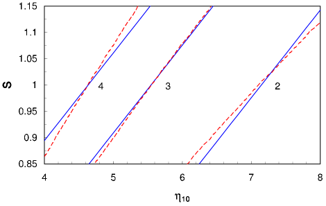
Figure 5: BBN-predicted isoabundance curves for D in the expansion-rate parameter ($S$), baryon density parameter ($\eta$) plane. From left to right, $y_{\rm D}$ = 4, 3, 2. The solid curves are the BBN-predicted results, while the dotted curves are our fits (see the text).

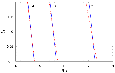
Figure 6: BBN-predicted isoabundance curves for D in the lepton asymmetry parameter ($\xi_{e}$), baryon density parameter ($\eta$) plane. From left to right, $y_{\rm D}$ = 4, 3, 2. The solid curves are the BBN-predicted results, while the dotted curves are our fits (see the text).

Over the restricted range in $\eta$ under study here, the deuterium abundance $y_{\rm D}$ $\equiv 10^{5}($D/H), is well described by a power law in $\eta$ with $y_{\rm D}$ $\propto\eta^{-1.6}$. For our adopted range of $\eta$, $y_{\rm D}$ = $y_{\rm D}(\eta$) is well fit by

$$y_{\rm D}^{FIT}\equiv 46.5\eta_{10}^{-1.6}.$$ (15)

While the true $y_{\rm D}$ – $\eta$ relation is not precisely a power law, for $4~{}\lower 2.58334pt\vbox{\hbox{$\buildrel\textstyle<\over{\sim}\ $}}\eta_{10}~{}\lower 2.58334pt\vbox{\hbox{$\buildrel\textstyle<\over{\sim}\ $}}8$, this fit is accurate to better than 1%, three times smaller than the $\sim 3\%$ BBN uncertainty estimated by BNT bnt ; this fit agrees with the BNT prediction to 2% or better over this range in $\eta$.

In analogy with $\eta_{\rm He}$ defined by the ⁴He abundance (eq. 12), it is useful to define a similar parameter, $\eta_{\rm D}$, for D (including a $3\%$ error estimate),

$$\eta_{\rm D}\equiv({46.5(1\pm 0.03)\over y_{\rm D}})^{1/1.6}.$$ (16)

Substituting the abundance estimate (§II) for primordial D into this equation leads to our adopted value for $\eta_{\rm D}=6.06^{+0.68}_{-0.53}$ ($\Omega^{\rm D}_{\rm B}h^{2}=0.0221^{+0.0025}_{-0.0019}$).

For the adopted ranges in $\eta$, $S$, and $\xi_{e}$, a simple linear relation which provides a good fit to $\eta_{\rm D}$ (see Figures 5 & 6) is,

$$\eta_{\rm D}=\eta_{10}-6(S-1)+{5\xi_{e}\over 4}.$$ (17)

As may be seen from Figures 5 & 6, this fit works quite well (for $4\leq\eta_{10}\leq 8$) for $2~{}\lower 2.58334pt\vbox{\hbox{$\buildrel\textstyle<\over{\sim}\ $}}y_{\rm D}~{}\lower 2.58334pt\vbox{\hbox{$\buildrel\textstyle<\over{\sim}\ $}}4$, corresponding to $5~{}\lower 2.58334pt\vbox{\hbox{$\buildrel\textstyle<\over{\sim}\ $}}\eta_{\rm D}~{}\lower 2.58334pt\vbox{\hbox{$\buildrel\textstyle<\over{\sim}\ $}}7$. Given the restricted ranges for $S$ and $\xi_{e}$, it is clear from Figures 5 & 6 and eq. 17 that D is a senstive baryometer ($\eta_{\rm D}\approx\eta_{10}$).

III.3 Helium-3

The dependence of the BBN-predicted abundance of ³He on the baryon density, expansion rate, and lepton asymmetry is similar to that of D but, ³He is considerably less sensitive to them than is D. Indeed, over the parameter ranges adopted here, the ³He abundance is well fit by $y_{3}\propto y_{\rm D}^{0.35}$. As a result, along with its more complicated post-BBN evolution, ³He provides complementary but less compelling constraints than does D. In our subsequent analysis, ³He is set aside in favor of D.

III.4 Lithium-7

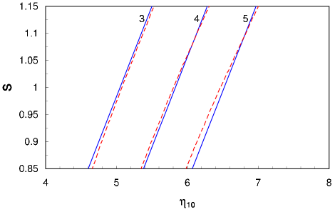
Figure 7: BBN-predicted isoabundance curves for ⁷Li in the expansion-rate parameter ($S$), baryon density parameter ($\eta$) plane. From left to right, $y_{\rm Li}$ = 3, 4, 5. The solid curves are the BBN-predicted results, while the dotted curves are our fits (see the text).

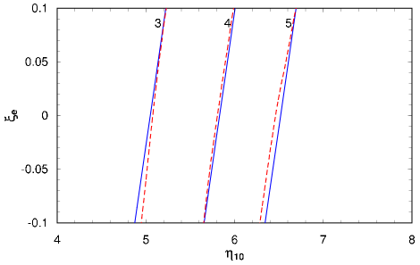
Figure 8: BBN-predicted isoabundance curves for ⁷Li in the lepton asymmetry parameter ($\xi_{e}$), baryon density parameter ($\eta$) plane. From left to right, ⁷Li, $y_{\rm Li}$ = 3, 4, 5. The solid curves are the BBN-predicted results, while the dotted curves are our fits (see the text).

As with D, the ⁷Li abundance is well described by a power law in $\eta$ over the range in baryon abundance explored here: $y_{\rm Li}$ $\equiv 10^{10}$(Li/H)$~{}\propto\eta^{2}$. The following fit agrees with the BBN predictions to better than 3% over the adopted range in $\eta$,

$$y_{\rm Li}^{FIT}\equiv{\eta_{10}^{2}\over 8.5}.$$ (18)

While this fit predicts slightly smaller lithium abundances compared to those of BNT bnt , the differences are at the 5-8% level, small compared to the BNT uncertainty estimates as well as those of Hata et al.  hata ($\sim 10-20\%$).

In analogy with $\eta_{\rm D}$ and $\eta_{\rm He}$ defined above, we introduce $\eta_{\rm Li}$ (allowing for a $10\%$ uncertainty), defined by,

$$\eta_{\rm Li}\equiv(8.5(1\pm 0.1)y_{\rm Li})^{1/2}.$$ (19)

Using the Ryan et al. ryan estimate (§II) $y_{\rm Li}$ $=1.23^{+0.34}_{-0.16}$, $\eta_{\rm Li}=3.23^{+0.44}_{-0.28}$ ($\Omega^{\rm Li}_{\rm B}h^{2}=0.0118^{+0.0016}_{-0.0010}$), while the Bonifacio et al. bonif result of $y_{\rm Li}$ $=2.19^{+0.46}_{-0.38}$ gives $\eta_{\rm Li}=4.31^{+0.48}_{-0.46}$ ($\Omega^{\rm Li}_{\rm B}h^{2}=0.0157\pm 0.0017$).

A simple, linear relation for $\eta_{\rm Li}$ as a function of $\eta$, $S$, $\xi_{e}$, which works reasonably well over the adopted parameter ranges (see Figures 7 & 8) is,

$$\eta_{\rm Li}=\eta_{10}-3(S-1)-{7\xi_{e}\over 4}.$$ (20)

As Figures 7 & 8 reveal, this fit works well (for $4\leq\eta_{10}\leq 8$) for $3~{}\lower 2.58334pt\vbox{\hbox{$\buildrel\textstyle<\over{\sim}\ $}}y_{\rm Li}~{}\lower 2.58334pt\vbox{\hbox{$\buildrel\textstyle<\over{\sim}\ $}}5$, corresponding to $5~{}\lower 2.58334pt\vbox{\hbox{$\buildrel\textstyle<\over{\sim}\ $}}\eta_{\rm Li}~{}\lower 2.58334pt\vbox{\hbox{$\buildrel\textstyle<\over{\sim}\ $}}7$. We note that this fit breaks down for $y_{\rm Li}$ $\lower 2.58334pt\vbox{\hbox{$\buildrel\textstyle<\over{\sim}\ $}}2$ ($\eta_{\rm Li}~{}\lower 2.58334pt\vbox{\hbox{$\buildrel\textstyle<\over{\sim}\ $}}4$). In addition, Figures 7 & 8, along with eq. 20, show that, as is the case for deuterium, lithium can be an excellent baryometer (for the restricted ranges of $S$ and $\xi_{e}$, $\eta_{\rm Li}\approx\eta_{10}$).

IV Applications

In this section the application of our simple, linear fits (among $\eta$, $S$, $\xi_{e}$, and y_D, y_Li, Y_P) is illustrated by considering several standard and nonstandard BBN options.

IV.1 SBBN

Figure 9: The baryon abundance parameters (see §III) corresponding to the D, ⁴He, and ⁷Li abundances adopted here (from §II), and from WMAP sperg

As a first application of our simple fits to the predicted primordial abundances, consider the case of SBBN ($S=1$, $\xi_{e}=0$). In this case the predicted abundances depend on only one adjustable parameter, the baryon abundance parameter $\eta$. For SBBN we may adopt the WMAP-inspired value sperg of $\eta_{10}=6.14\pm 0.25$ ($\Omega_{\rm B}h^{2}\;$$=0.0224\pm 0.009$). For $S=1$ and $\xi_{e}$ = 0 we expect,

$$SBBN:~{}\eta_{\rm D}=\eta_{\rm He}=\eta_{\rm Li}=\eta_{10}.$$ (21)

It is clear from Figure 9, using the abundances identified in §II, that eq. 21 is not satisfied ($\eta_{\rm D}\approx\eta_{10}\neq\eta_{\rm He}\approx\eta_{\rm Li}$). However, SBBN does work for deuterium: $\eta_{\rm D}=6.06^{+0.68}_{-0.53}\approx\eta_{10}=6.14\pm 0.25$. In addition, we note that for the WMAP baryon abundance the SBBN-predicted value of the ³He primordial abundance, $1.1\pm 0.1\times 10^{-5}$, is in excellent agreement with that inferred from the study of Galactic H $\scriptstyle{\rm II}$ regions rood . The problems arise for ⁴He and ⁷Li.

For ⁴He, the recent Izotov & Thuan it04 determination of the primordial mass fraction leads to $\eta_{\rm He}=2.81\pm 0.68$ (§IIIA), which is $\sim 6\sigma$ below the WMAP baryon density parameter. While Izotov & Thuan have attempted to account for some of the potential systematic errors in their Y_P determination, it may well be that they have underestimated the residual error; see, e.g., Olive and Skillman os04 . If not, this disagreement may provide a hint of new physics beyond the standard model ($S\neq 1$ and/or $\xi_{e}\neq 0$).

As may be seen from Figures 1, 2, 4, & 7, along with eqs. 16 & 19, the BBN-predicted abundance of ⁷Li is closely tied to that of D, y${}_{\rm Li}\approx 4.3(y_{\rm D}/2.6)^{-5/4}$. For y_D in its observed range (and/or for $\eta_{10}$ in the WMAP range), y${}_{\rm Li}\approx 4-5$ ([Li]  $\approx 2.6-2.7$). For the WMAP baryon abundance the SBBN prediction is y${}_{\rm Li}=4.44^{+0.58}_{-0.57}$, to be compared with the halo star estimate from Ryan et al.  ryan of y${}_{\rm Li}=1.23^{+0.34}_{-0.16}$, or with the globular cluster estimate from Bonifacio et al.  bonif of y${}_{\rm Li}=2.19^{+0.46}_{-0.38}$. The SBBN-predicted ⁷Li abundance is much higher, by factors of $\sim 2-4$, than those inferred from the studies of the oldest halo and/or globular cluster stars in the Galaxy. It will be seen in more detail below that it is unlikely that any of the “simple” nonstandard effects ($S\neq 1$, $\xi_{e}\neq 0$) can resolve this conflict (since the ⁷Li and D abundances are so tightly coupled). It may well be that for these oldest stars in the Galaxy, mixing surface material with the lithium-depleted interior has reduced their observed, surface lithium abundances from the primordial value pwsn ; pswn .

IV.2 Non-Standard Expansion: $S\neq 1$, $\xi_{e}=0$

The previous section has reminded us of the tension between the observationally-inferred primordial abundances of D, ⁴He, and ⁷Li; see, e.g., osw . While it is not unlikely that the resolution of these conflicts may be found in systematic uncertainties of the astronomy (e.g., corrections to the derived helium abundance and/or lithium depletion/dilution via mixing), they may be providing hints of new physics. Since the BBN abundance of ⁴He is sensitive to the early-Universe expansion rate and that of D probes the baryon density, a combination of the two abundances permits us to investigate constraints on models with non-standard expansion rates  ssg ; ossw . Setting aside ⁷Li for the moment and only using D and ⁴He, we may use equations 13 and 16 to find

$$S-1={\eta_{\rm He}-\eta_{\rm D}\over 106}$$ (22)

and,

$$\eta_{10}={100\eta_{\rm D}+6\eta_{\rm He}\over 106}.$$ (23)

It is clear from eq. 23 that D is the dominant baryometer. While it may appear from eq. 22 that D and ⁴He make comparable contributions to constraining the expansion rate, recall that $\eta_{\rm He}$ is linear in Y_P while $\eta_{\rm D}$ varies only as a fractional power of y_D. Thus, whereas reconciling Y_P with y_D requires an increase in Y_P of $\Delta$Y${}_{\rm P}\approx 0.006$ ($\sim 2.5\%$), reconciling D with ⁴He would require that y_D increase by a factor of $\sim 4-5$ (and, the resulting $\eta_{\rm D}$ would then be in conflict with the WMAP determination of $\eta_{10}$). From eq. 22, for $\Delta$N${}_{\nu}\ll 1$ and with y_D ($\eta_{\rm D}$) fixed, $\Delta$Y$~{}\approx 0.014\Delta$N_ν. Note that depending on the quantity held fixed ($\eta_{10}$ or $\eta_{\rm D}$), the coefficients in the $\Delta$Y – $\Delta$N_ν relations differ slightly.

For the values adopted in §IIIA,B (and their uncertainties), $\eta_{\rm D}=6.06^{+0.68}_{-0.53}$ and $\eta_{\rm He}=2.81\pm 0.68$, we find

$$\eta_{10}=5.88^{+0.64}_{-0.50}\ \ ;\ \ S=0.969^{+0.008}_{-0.009}.$$ (24)

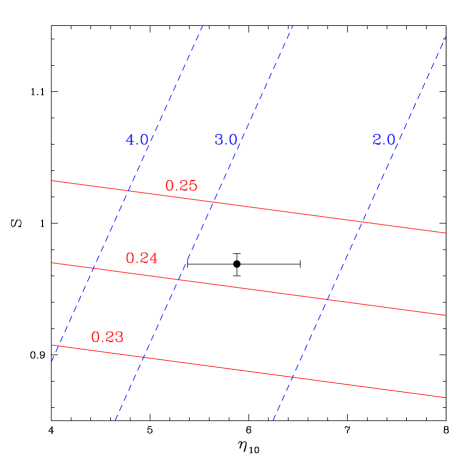
Figure 10: BBN-predicted isoabundance curves for D (dashed) and ⁴He (solid) in the expansion-rate parameter ($S$), baryon density parameter ($\eta$) plane. The point with error bars corresponds to the adopted abundances for D and ⁴He ($\xi_{e}=0$); see the text, eq. 23.

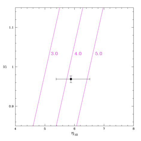
Figure 11: BBN-predicted isoabundance curves ⁷Li in the expansion-rate parameter ($S$), baryon density parameter ($\eta$) plane. The numbers next to the curves are for y_Li. The point with error bars corresponds to the adopted abundances for D and ⁴He ($\xi_{e}=0$) as in Figure 9.

If the non-standard expansion rate factor is associated with an equivalent number of neutrinos, $\Delta$N${}_{\nu}=-0.37^{+0.10}_{-0.11}$. These results, along with the D and ⁴He isoabundance curves, are shown in Figure 10. Notice that although $\Delta N_{\nu}\;$is now closer to zero than in, e.g.,  barger03a , the smaller adopted uncertainty in Y_P results in a larger, $\sim 3-4\sigma$ discrepancy. However, these BBN results for the baryon density and the expansion rate are in excellent agreement with those from WMAP which, while sensitive to the baryon density parameter is relatively insensitive to the expansion rate factor; see barger03a .

Although the above combination of $\eta_{10}$ and $S$ can reconcile the inferred primordial abundances of D and ⁴He, it cannot resolve the lithium problem.

$$\eta_{\rm Li}={103\eta_{\rm D}+3\eta_{\rm He}\over 106}=5.97^{+0.66}_{-0.52}.$$ (25)

Accounting for the theoretical uncertainty in the BBN lithium production and in our fit,

$${\rm y}_{\rm Li}=4.20^{+1.07}_{-0.81}\ \ ;\ \ [{\rm Li}]_{\rm P}=2.62^{+0.10}_{-0.09}.$$ (26)

This conflict is shown in Figure 11 where the D and ⁴He constraints on $\eta_{10}$ and $S$ are shown along with isoabundance curves for ⁷Li. It is clear that y${}_{\rm Li}<3$ is strongly disfavored.

IV.3  Non-Zero Lepton Number: $\xi_{e}\neq 0$, $S=1$

In an attempt to relieve the tension between the BBN predicted and observed deuterium and helium-4 abundances, a non-zero lepton number ($\nu_{e}-\bar{\nu}_{e}$ asymmetry; $\xi_{e}\neq 0$) is an alternative to the non-standard expansion rate explored in the previous section. An excess of $\nu_{e}$ over $\bar{\nu}_{e}$ will drive down the pre-BBN neutron-to-proton ratio, leaving fewer neutrons to be incorporated in ⁴He. The resulting, lower, BBN-predicted ⁴He abundance will be closer to that observed. At the same time, the effect of an e-neutrino asymmetry on the abundances of D and/or ⁷Li is small.

As for the case of $S\neq 1$, we set aside ⁷Li and use D and ⁴He to constrain $\eta_{10}$ and $\xi_{e}$. For $S=1$,

$$\eta_{10}={115\eta_{\rm D}+\eta_{\rm He}\over 116}$$ (27)

and,

$$\xi_{e}={\eta_{\rm D}-\eta_{\rm He}\over 145}.$$ (28)

Using the D and ⁴He abundances adopted here,

$$\eta_{10}=6.04^{+0.67}_{-0.53}\ \ ;\ \ \xi_{e}=0.022^{+0.007}_{-0.006}$$ (29)

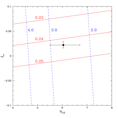
Figure 12: BBN-predicted isoabundance curves for D (dashed) and ⁴He (solid) in the lepton asymmetry parameter ($\xi_{e}$), baryon density parameter ($\eta$) plane. The point with error bars corresponds to the adopted abundances for D and ⁴He ($S=1$); see the text, eq. 28.

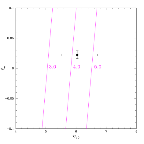
Figure 13: BBN-predicted isoabundance curves ⁷Li in the lepton asymmetry parameter ($\xi_{e}$), baryon density parameter ($\eta$) plane. The numbers next to the curves are for y_Li. The point with error bars corresponds to the adopted abundances for D and ⁴He ($S=1$) as in Figure 11.

These results, along with the D and ⁴He isoabundance curves, are shown in Figure 12.

A “small” lepton asymmetry, $\xi_{e}\approx 0.02$, which, however, is very large compared to the baryon asymmetry ($\sim\eta~{}\lower 2.58334pt\vbox{\hbox{$\buildrel\textstyle<\over{\sim}\ $}}10^{-9}$), can reconcile the observationally inferred primordial D and ⁴He abundances with the predictions of BBN. But, this lepton asymmetry will not resolve the conflict between the BBN-predicted and observed ⁷Li abundances since

$$\eta_{\rm Li}={142\eta_{\rm D}+3\eta_{\rm He}\over 145}=5.99^{+0.67}_{-0.52}$$ (30)

and,

$${\rm y}_{\rm Li}=4.23^{+1.08}_{-0.82}\ \ ;\ \ [{\rm Li}]_{\rm P}=2.63^{+0.10}_{-0.09}.$$ (31)

As is the case for a non-standard expansion rate, the BBN-predicted abundance of ⁷Li is very tightly tied to that of D, and a non-zero lepton number cannot resolve the conflict between theory and data. This is illustrated in Figure 13, where it is clear that here, too, y${}_{\rm Li}<3$ is strongly disfavored.

IV.4 Non-Zero Lepton Number ($\xi_{e}\neq 0$) And Non-Standard Expansion Rate ($S\neq 1$; N${}_{\nu}\neq 3$)

In §IVB it was seen that, in the absence of a non-zero lepton number, the D and ⁴He abundances severely restrict deviations of the early universe expansion rate from its standard value. When associated with the effective number of neutrinos, this constraint (for the choice of D and ⁴He abundances adopted here) is nearly $4\sigma$ away from the standard value of N${}_{\nu}=3$. If the LSND result lsnd is interpreted in terms of a 4th, “sterile”, neutrino, the mixing of such a neutrino with the active neutrinos would bring it into equilibrium in the early universe prior to BBN volkas , resulting in N${}_{\nu}=4$ at BBN. Clearly (see §IIIB), the current best estimates of the primordial abundances cannot tolerate the corresponding speed-up in the expansion rate at BBN. However, in §IIIC it was shown that N${}_{\nu}=3$ is perfectly acceptable provided that there is a small but significant $\nu_{e}-\bar{\nu}_{e}$ asymmetry. It is, therefore, not unexpected that for $\xi_{e}\neq 0$, the BBN constraints on $S$ ($\Delta$N_ν) are considerably expanded (see, e.g., Barger et al. barger03a and references therein). In implementing for BBN $S\neq 1$ as well as $\xi_{e}\neq 0$, there is a problem. Because of concerns about the primordial ⁷Li (and ³He) abundances as inferred from current observational data, the analysis here has been restricted to employing only the D and ⁴He abundances. But, with three free parameters ($\eta_{10}$, $S$ (or $\Delta$N_ν), and $\xi_{e}$) and only two constraints ($\eta_{\rm D}$ and $\eta_{\rm He}$), non-BBN data (restricting $\eta_{10}$) is required to proceed further. Retaining the constraints from D and ⁴He, $S$ and $\xi_{e}$ are then functions of the baryon density parameter.

$$590(S-1)=116\eta_{10}-(115\eta_{\rm D}+\eta_{\rm He})$$ (32)

and,

$$145\xi_{e}=106(S-1)+\eta_{\rm D}-\eta_{\rm He}.$$ (33)

For the abundances adopted here (§II), this leads to

$$590(S-1)=116\eta_{10}-700^{+78}_{-61},$$ (34)

and

$$\xi_{e}=0.731(S-1)+0.0224^{+0.0066}_{-0.0059}.$$ (35)

This $\xi_{e}$ – $S$ relation is shown in Figure 14.

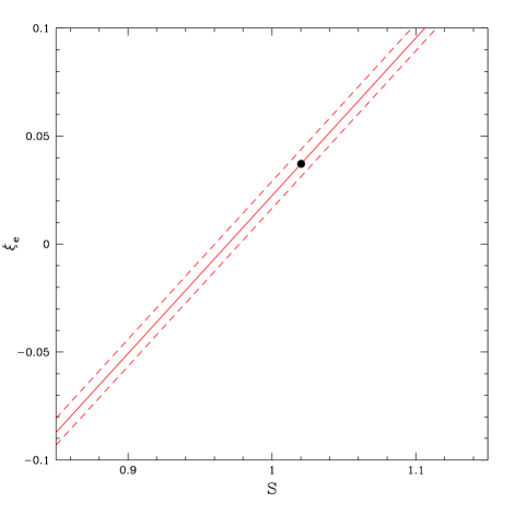
Figure 14: BBN-predicted $\xi_{e}-S$ relation corresponding to the adopted D and ⁴He abundances. The solid curve is for the central value and the dashed curves represent the $1\sigma$ uncertainties. The point indicated corresponds to the WMAP value for the baryon density; see the text.

A constraint on the baryon density is possible utilizing CBR data provided that the corresponding values of $S-1$ and $\xi_{e}$ are sufficiently small, so that the expansion rate at recombination, some 400 kyr after BBN, doesn’t deviate significantly from the standard value. For the WMAP recommended baryon abundance sperg , $\eta_{10}=6.14$, $S\approx 1.0203$, corresponding to $\Delta$N${}_{\nu}\approx 0.25$ and $\xi_{e}\approx 0.037$. This point is shown in Figure 14.

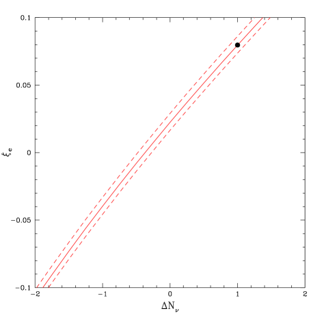
Figure 15: BBN-predicted $\xi_{e}-\Delta$N_ν relation corresponding to the adopted D and ⁴He abundances. The solid curve is for the central value and the dashed curves represent the $1\sigma$ uncertainties. The point indicated corresponds to N${}_{\nu}=4$.

It is now possible to address the question of whether or not BBN permits N${}_{\nu}=4$ ($S=1.0783$). This choice for $S$ requires $\xi_{e}=0.080$ and $\eta_{10}=6.43$, only $\sim 1\sigma$ away from the WMAP value. This point is shown in Figure 15 where the $\xi_{e}-\Delta$N_ν relation is displayed. While BBN constraints on more extreme cases (e.g., $\Delta$N${}_{\nu}~{}\lower 2.58334pt\vbox{\hbox{$\buildrel\textstyle>\over{\sim}\ $}}2$) can be explored (see, e.g., Barger et al.  barger03b ), our simple fits begin to become inaccurate for $\xi_{e}~{}\lower 2.58334pt\vbox{\hbox{$\buildrel\textstyle>\over{\sim}\ $}}0.1$, limiting our analysis here to $\Delta$N${}_{\nu}~{}\lower 2.58334pt\vbox{\hbox{$\buildrel\textstyle<\over{\sim}\ $}}1.2$ (see Figure 15).

For the general case studied here, the BBN-predicted lithium abundance depends on the baryon density (as well as on the D and ⁴He abundances).

$$\eta_{\rm Li}=0.159\eta_{10}+0.822\eta_{\rm D}+0.019\eta_{\rm He}.$$ (36)

Notice that here, too, the ⁷Li abundance is tightly tied to that of D. Indeed,

$$\eta_{\rm Li}=\eta_{\rm D}+3[(S-1)-\xi_{e}]\approx\eta_{\rm D}.$$ (37)

As before, there are lithium “problems” for the two cases studied above. For the WMAP combination of parameters (see eq. 19), $\eta_{\rm Li}=6.01$, so that $y_{\rm Li}$ = 4.25 ([Li] = 2.63). For N${}_{\nu}=4$, $\eta_{\rm Li}=6.06$, corresponding to $y_{\rm Li}$ = 4.32 ([Li] = 2.64). At least for these combinations of non-standard physics (as well as for SBBN), there is an apparent conflict between the BBN predicted and observed primordial abundances of lithium.

V Summary And Conclusions

In the toolbox of a particle phenomenologist, BBN is a venerable and valuable tool, providing complementary constraints on – or hints of – new physics beyond the standard model. As the models change and the data are updated, not every phenomenologist on the street may have easy access to a BBN code to enable quick revision of previous bounds or investigation of new hints. It may, then, be of value to have simple fits to the BBN-predicted abundances as functions of the key variables (baryon density, expansion rate or neutrino number, neutral lepton asymmetry). For interesting but limited ranges of the parameters such fits have been presented here and applied to several simple examples. We have seen that the observed D and ⁴He abundances, while apparently inconsistent with SBBN (modulo systematic errors in the data), can be reconciled if non-standard expansion rates and/or non-zero lepton number are allowed. It was also shown how non-zero lepton number allows one – or more – sterile neutrinos while maintaining the consistency of BBN. Finally, by revealing the clear connections between the BBN-predicted abundances of D and ⁷Li, we showed that none of these non-standard physics solutions can reconcile the observed and predicted lithium abundances.

References

- (1) S. M. Carroll and M. Kaplinghat, Phys. Rev. D, 65, 063507 (2002).
- (2) E. Massó and F. Rota, Phys. Rev. D, 68, 123504 (2003).
- (3) J. P. Kneller and G. Steigman, Phys. Rev. D, 67, 063501 (2003).
- (4) J. D. Barrow and R. J. Scherrer, [astro-ph/0406088], (2004)
- (5) A. Serna, R. Dominguez-Tenreiro and G. Yepes, ApJ, 391, 433 (1992).
- (6) A. Serna and R. Dominguez-Tenreiro, Phys. Rev. D, 48, 1591 (1993).
- (7) R. Bean, S. H. Hansen and A. Melchiorri, Phys. Rev. D, 64, 103508 (2001)
- (8) D. N. Spergel, et al. , ApJS, 148, 175 (2003)
- (9) V. Barger, J. P. Kneller, D. Marfatia, P. Langacker, and G. Steigman, Phys. Lett. B, 569, 123 (2003).
- (10) V. Barger, J. P. Kneller, H.-S. Lee, D. Marfatia, and G. Steigman, Phys. Lett. B, 566, 8 (2003).
- (11) G. Steigman, D. N. Schramm, and J. E. Gunn, Phys. Lett. B, 66, 202 (1977).
- (12) L. Randall and R. Sundrum, Phys. Rev. Lett. 83, 3370 (1999); Phys. Rev. Lett. 83, 4690 (1999).
- (13) H. S. Kang and G. Steigman, Nucl. Phys. B, 372, 494 (1992).
- (14) J. P. Kneller, R. J. Scherrer, G. Steigman, and T. P. Walker, Phys. Rev. D, 64, 123506 (2001).
- (15) C. Lunardini and A. Y. Smirnov, Phys. Rev. D, 64, 073006 (2001); A. D. Dolgov, S. H. Hansen, S. Pastor, S. T. Petcov, G. G. Raffelt and D. V. Semikoz, Nucl. Phys. B, 632, 363 (2002); Y. Y. Wong, Phys. Rev. D, 66, 025015 (2002); K. N. Abazajian, J. F. Beacom and N. F. Bell, Phys. Rev. D, 66, 013008 (2002).
- (16) S. Burles, K. M. Nollett, and M. S. Turner, Phys. Rev. D, 63, 063512 (2001).
- (17) N. Hata, R. J. Scherrer, G. Steigman, D. Thomas, T. P. Walker, S. Bludman, and P. Langacker, Phys. Rev. Lett., 75, 3977 (1995).
- (18) R. Epstein, J. Lattimer, and D. N. Schramm, Nature 263, 198 (1976).
- (19) T. M. Bania, R. T. Rood, and D. Balser, Nature, 415, 54 (2002).
- (20) S. Burles and D. Tytler, ApJ, 499, 699 (1998a).
- (21) S. Burles and D. Tytler, ApJ, 507, 732 (1998b).
- (22) J. M. O’Meara, et al. , ApJ, 552, 718 (2001).
- (23) M. Pettini, and D. V. Bowen, ApJ, 560, 41 (2001).
- (24) S. D’Odorico, M. Dessauges-Zavadsky, and P. Molaro, A&A, 338, L1 (2001).
- (25) D. Kirkman, D. Tytler, N. Suzuki, J. O’Meara, and D. Lubin, ApJS, 149, 1 (2003)
- (26) G. Steigman, STScI Symposium Series, 15, 46 (2004); Proceedings of the May 2001 STScI Symposium, ”The Dark Universe: Matter, Energy, and Gravity”, ed. M. Livio.
- (27) Y. I. Izotov, T. X. Thuan, and V. A. Lipovetsky, ApJS, 108, 1 (1997).
- (28) Y. I. Izotov, T. X. Thuan, and V. A. Lipovetsky, ApJ, 500, 188 (1998).
- (29) K. A. Olive and G. Steigman, ApJS, 97, 49 (1995).
- (30) K. A. Olive, E. Skillman, and G. Steigman, ApJ, 483, 788 (1997).
- (31) B. D. Fields and K. A. Olive, ApJ, 506, 177 (1998).
- (32) Y. I. Izotov and T. X. Thuan, ApJ, 602, 200 (2004).
- (33) K. A. Olive and E. D. Skillman, [astro-ph/0405588], (2004).
- (34) S. G. Ryan, T. C. Beers, K. A. Olive, B. D. Fields, and J. E. Norris, ApJL, 530, L57 (2000).
- (35) P. Bonifacio and P. Molaro, MNRAS, 285, 847 (1997); P. Bonifacio, P. Molaro, and L. Pasquini, MNRAS, 292, L1 (1997).
- (36) M. H. Pinsonneault, T. P. Walker, G. Steigman, and V. K. Narayanan, ApJ, 527, 180 (1999).
- (37) M. H. Pinsonneault, G. Steigman, T. P. Walker, & V. K. Narayanan, ApJ, 574, 574, 398 (2002).
- (38) K. A. Olive, G. Steigman & T. P. Walker, Phys. Rep., 333, 389 (2000).
- (39) K. A. Olive, D. N. Schramm, G. Steigman, and T. P. Walker, Phys. Lett. B, 236, 454 (1990).
- (40) A. Aguilar et al. [LSND Collaboration], Phys. Rev. D, 64, 112007 (2001).
- (41) R. Foot and R. R. Volkas, Phys. Rev. Lett. 75, 4350 (1995).