Star Formation in Hi Selected Galaxies I: Sample Characteristics

Abstract

A sample of 69 galaxies with radial velocities less than 2500 km s^-1 was selected from the Hi Parkes All Sky Survey (HiPASS) and imaged in broad band B and R and narrow band H$\alpha$ to deduce details about star formation in nearby disk galaxies while avoiding surface brightness selection effects. The sample is dominated by late-type, dwarf disks (mostly Sc and Sm galaxies) with exponential disk scale lengths $\sim$1 to 5 kpc. The HiPASS galaxies on average have lower star formation rates (SFRs) and are bluer and lower surface brightness than an optically selected sample. Hii regions were detected in all but one of the galaxies. Many galaxies had as few as two to five Hii regions. The galaxies’ H$\alpha$ equivalent widths, colors, and SFRs per unit Hi mass are best explained by young mean ages ($\sim$3 to 5 Gyr according to Schmidt Law models) with star formation histories where the SFRs were higher in the past. Comparison of the surface brightness coverage of the HiPASS galaxies with that of an optically selected sample shows that such a sample may miss $\sim$10% of the local galaxy number density and could possibly miss as much as 3 to 4% of the SFR density. The amount lower surface brightness galaxies contribute to the total luminosity density may be insignificant, but this conclusion is somewhat dependent on how the fluxes of these objects are determined.

1 Introduction

Ground based optical observations of galaxies have traditionally suffered from the inevitable bias toward higher surface brightness produced by the intensity of the night sky. Of course, this bias is still a problem, but its effect has been lessened by the advent of more sensitive detectors and the use of larger and better optical systems. Consequently, in recent years so called low surface brightness (LSB) galaxies have become a topic of great interest. These previously overlooked members of the galaxy population have since been shown to be larger at the same luminosity as high surface brightness (HSB) galaxies (de Blok et al., 1996) while still obeying the same Tully-Fisher relationship, but only if the entire baryonic content of the galaxies is taken into account (McGaugh et al., 2000). LSB disks also tend to be less dense and more metal poor (de Blok & van der Hulst, 1998) and have higher gas mass fractions than HSB disks (McGaugh & de Blok, 1997). In addition, attempts at detecting molecular gas in LSB galaxies have been fairly unsuccessful; only 3 out of 34 LSB galaxies observed at the $J$(1-0) and $J$(2-1) CO lines have been found to contain a detectable amount of CO emission (O’Neil, Schinnerer, & Hofner, 2003). Considering these observational trends, it is uncertain whether the characteristics of a sample of galaxies selected according to optical properties would accurately reflect those of the entire galaxy population.

Among the galaxy characteristics of particular interest in the optical regime are those that relate to star formation. Given that the typical LSB galaxy has a metallicity of $\sim\frac{1}{3}$ solar (McGaugh, 1994), the lack of detections of CO emission may not be definitive evidence for extremely low amounts of molecular gas in LSB disks, as the CO to H₂ relation tends to break down for metallicities $\sim\frac{1}{2}$ solar and lower. Still, the lack of detections, when taken into consideration with LSB disks’ low metallicities and Hi surface densities that are often near or below the critical limit for star formation (de Blok et al., 1996; Kennicutt, 1989), imply that these galaxies should not be forming very many stars. In fact, observations show that the typical LSB disk has a star formation rate that is about ten times lower than the average rate for HSB disks (Mihos et al., 1999). Despite this, LSB disks tend to be relatively blue and several have been observed to contain a number of prominent Hii regions. The fact that the majority of known LSB disks are bluer might be the result of a selection bias; a fair number of redder LSB galaxies have recently been detected (O’Neil et al., 2000). However, the fact that there are so many nearby LSB galaxies that are quite blue along with the presence of Hii regions suggests that it is very possible for high mass stars to form in such unfavorable conditions. This implies that LSB disks may not be characterized simply as less dense and less productive versions of their HSB counterparts and that it is possible that their star formation histories could be much different.

A sample of galaxies selected from a single dish Hi survey will be mainly limited by the total neutral gas content of the galaxies; there is no explicit bias due to surface brightness or Hi column density. Therefore, the existence of any fundamental differences between the star formation histories in LSB and HSB galaxies and the relative contribution to the amount of local star formation made by LSB galaxies might be revealed by comparing the star formation properties of a neutral hydrogen selected sample to those of a sample chosen from an optical catalog. The purpose of this and a subsequent paper is to examine the results of broad band B and R and narrow band H$\alpha$ imaging of a nearby sample of galaxies chosen from the Hi Parkes All Sky Survey (HiPASS) (Barnes et al., 2001) in order to derive information about the galaxies’ star formation histories and to compare the results with those from an optically selected sample. This paper discusses the initial results of the data acquisition and reduction, the basic observational properties of each galaxy, and trends among the sample.

2 Data Acquisition, Reduction, and Calibration

2.1 Sample Selection, Observations, and Reduction

The galaxies that were imaged were chosen from a sample of all HiPASS galaxies with declinations $<$ -65^∘ and radial velocities $<$ 2500 km s^-1, 132 galaxies in all. Due mainly to weather constraints, 69 of these 132 were imaged. Because of extinction issues, lower priority was given to galaxies that appeared nearly edge-on on their Digitized Sky Survey images available through the NASA/IPAC Extra Galactic Database (NED). Because of this, we poorly sample the more highly inclined portion of the disk population. The effect of this on our analysis is discussed in Sec. 4.2. Data was acquired during two separate observing runs. During both runs, images were obtained at Cerro Tololo Inter-American Observatory (CTIO) utilizing the 0.9 m telescope and the Tek 2kx2k CCD camera, one on March 3 - 9, 2000 and the other on Oct. 23-28, Nov. 2, 5, 6, 2000. Conditions were photometric for all but one of the nights during the first run. Three of the eight nights of the second run were not photometric; during two of these nights, no images were obtained. All but three of the HiPASS galaxies observed had well known optical counterparts. Each galaxy was imaged twice through broad band B and R filters and a narrow band H$\alpha$ filter. In addition to the 3 in., 75 Å H$\alpha$ filters available at CTIO, 4 in., 30 Å filters kindly provided by Richard Rand were used during both runs. Standard IRAF routines in the CCDRED package were used to perform the flat fielding and trimming of the images as well as the overscan corrections.

2.2 Calibration

Photometric and spectrophotometric standard stars were imaged during both runs through all filters. The photometric standard fields were taken from Landolt (1992); the spectrophotometric standards were obtained from Stone & Baldwin (1983) and Baldwin & Stone (1984) (see Table 2 for a list of the fields used as they are identified in these references). Values for the atmospheric extinction coefficient, $k$, the transformation coefficient, $t$, and the zero point offset, $z$, were obtained by fitting the function $m_{inst}-m_{filter}=k_{filter}X+t_{filter}(B-R)+z_{filter}$ to the observed and published standard star data where $X$ is the airmass of the observation; for this paper, $m_{inst}=-2.5\mbox{log}(\frac{DN}{\tau})+25$ where $DN$ is the counts from the object and $\tau$ is the exposure time. For the H$\alpha$ images, the magnitudes of the spectrophotometric standards over the bandpasses of the filters used were calculated using the filter specifications and the magnitude of each star as a function of wavelength, $m_{\lambda}$, quoted in the above references where

$$m_{\lambda}=-2.5log(F_{\lambda})-21.1$$ (1)

with $F_{\lambda}$ in units of ergs s^-1 cm^-2 $\mbox{\AA}^{-1}$. These were then compared to the instrumental magnitudes to derive an extinction coefficient and zero point offset for each filter.

Standard star images were only obtained two to three times per night. Consequently, values for $k$, $t$, and $z$ were obtained for each run instead of each night so that a larger range in airmass values could be used in each fit (see Table 3 for a listing of the values derived for these parameters). Conditions on the sixth night of the March observing run and the eighth night of the October/November run were not photometric. The calibration of images taken on these nights is uncertain and the fluxes obtained should be taken as estimates only. Each galaxy that was observed on one of these nights is flagged with an $\ast$ in Tables 4, 5, and 6.

The galaxy images were corrected for cosmic rays by combining and averaging the pairs of images obtained in each bandpass. The continuum emission was subtracted from the H$\alpha$ images using the combined R-band images. To do this, the R-band images were scaled such that on average, the flux from foreground stars match that on the H$\alpha$ images. No attempt was made to correct for the presence of emission lines in the R bandpass for the galaxies. Therefore, this method may slightly overestimate the level of galaxy continuum emission on each H$\alpha$ image. However, the emission line equivalent widths for typical star forming disk galaxies lie between about 10 and 100 Å (e. g. Kennicutt, 1983), implying that for the R-band filter which has a FWHM of $\sim$1000 Å, the presence of emission lines will cause the continuum level to be off by only about 1 to 10% which is less than or approximately equal to the typical uncertainty for the zero points for the H$\alpha$ filters ($\sim$0.1 mag.).

Following sky subtraction, for each galaxy the B-R color was solved for using an estimate of the B and R instrumental magnitudes according to the following,

$$B-R=\frac{(m_{B}-m_{R})_{inst}-(k_{B}X_{1}-k_{R}X_{2})-(z_{B}-z_{R})}{1+t_{B}-t_{R}}$$ (2)

Each combined B and R and continuum subtracted H$\alpha$ image was then then divided by its exposure time and multiplied by 10${}^{0.4[k_{filter}X+t_{filter}(B-R)+z_{filter}-25]}$ where $t_{H\alpha}$=0.

Due to the larger number of H$\alpha$ filters used, fewer spectrophotometric standard star observations were made through each filter on the sixth night of the October/November run than on previous nights, and no reasonable results for the calibration coefficients could be obtained. In addition, only the 75Å CTIO H$\alpha$ filters were available during the previous nights whereas on the sixth night, the 30 Å Rand filters were used. Therefore, the calibration coefficients for the previous nights could not be used, and the calibration of the H$\alpha$ data for this night was performed using the R-band data in the following manner. It was assumed that the average monochromatic flux across the R filter, $F_{R}$, is proportional to the average monochromatic flux of the continuum across the H$\alpha$ filter, $F_{c}$, according to $F_{R}=C\cdot F_{c}$, which gives the following,

$$m_{c}=m_{R}+2.5log(C)+0.5$$ (3)

where $m_{R}$ is the magnitude in the R-band, $m_{c}=-2.5log(F_{c})-21.1$, and the average monochromatic flux and magnitude of Vega in the R-band are taken to be 2.15$\times$10^-9 ergs s^-1 cm^-2 $\mbox{\AA}^{-1}$ and 0.07 respectively. The raw counts from the R-band image, $DN_{R}$, are related to the counts from the continuum across the H$\alpha$ filter, $DN_{c}$, by a scale factor, $a$, that is determined during the continuum subtraction process, i. e. $DN_{R}=a\cdot DN_{c}$. The difference between the calibrated and instrumental magnitudes, $\Delta m$, for the H$\alpha$ filter can then be related to that for the R filter by the following,

$$\Delta m_{H\alpha}=\Delta m_{R}+2.5log(C\cdot a\cdot\frac{\tau_{R}}{\tau_{H\alpha}})+0.5$$ (4)

where $\tau$ is the exposure time. A mean value of $C$=0.73$\pm$0.15(1$\sigma$) was derived from the data from both runs that were calibrated with standard stars (see Fig. 1); a value of $C$=0.73 was used in the calibration of the remaining data. Given that all the data from the eighth night of the October/November run was calibrated using the standard star data from the sixth night of that run, the H$\alpha$ fluxes for galaxies imaged on that night were calibrated in this manner as well. Each galaxy whose H$\alpha$ flux was derived in this way is denoted by a $\star$ in table 6.

3 Photometric Measurements

3.1 Isophotal and Surface Photometry

After the combined B and R and H$\alpha$ continuum subtracted images were constructed and calibrated, isophotal photometry was performed on the galaxies in the following manner. On the calibrated B-band image, the 25 mag arcsec.^-2 isophote was identified by smoothing the image with a 7 pixel wide boxcar and then locating all pixels within 3$\sigma_{cal}$ of 25 mag arcsec.^-2, where $\sigma_{cal}$ is the uncertainty in the flux due to the error in the calibration. The width of the boxcar was chosen to be big enough to remove noise features from each image without eliminating the basic shape of the galaxy’s surface brightness profile (7 pixels corresponds to about 0.5 kpc for $V_{R}$=2500 km s^-1). These pixels were fit with an ellipse to determine the center, ellipticity, and position angle of the 25 mag arcsec.^-2 isophote; a polygon aperture was then drawn around these pixels to isolate the galaxy on the image. A pixel mask was created by replacing all pixels with fluxes greater than or equal to 25 mag arcsec.^-2 with values of unity and the rest with values of zero. For each galaxy, all three images were multiplied by this mask and the fluxes within the polygon aperture for the resulting images were measured to obtain isophotal magnitudes in all three bands. The mask was then used to estimate the isophotal radius for the object; this radius was taken to be the radius of a circle with the same area as the space occupied by all of the non-zero pixels on the mask image that were within the polygon aperture. These radii are reported in Table 4 along with estimates for the position angles and inclinations for the galaxies based on the shapes of the 25 mag. arcsec.^-2 isophotes. The isophotal magnitudes are contained in Table 4 as well. For each measured flux, the uncertainty was computed and was found to be dominated by the uncertainty in the calibration coefficients; the mean error for the fluxes is approximately the same for both bands and is equal to $\sim$0.045 mag.

For one galaxy, ESO035-G009, the observed surface brightness in the center of the object on the B-band image was approximately 25 mag arcsec.^-2. Therefore, a 25 mag arcsec.^-2 isophote could not be identified. The B-band image was sufficiently deep (the exposure time used was twice the typical time used for the rest of the galaxies) that a 26 mag arcsec.^-2 isophote could be identified. Therefore the isophotal quantities reported for this galaxy are for the 26 mag arcsec.^-2 isophote; the galaxy is flagged with a ${\dagger}$ in Table 4.

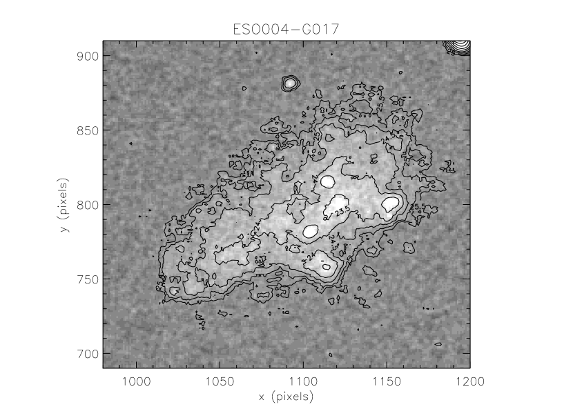
Figure 3: B-band image of ESO004-G017, an Sm galaxy, with contours drawn for different isophotes; the surface brightness of each isophote is given in mag arcsecond^-2. Note that there are three discrete 23.5 mag arcsecond^-2 isophotes caused by irregularly distributed Hii regions; the 24 mag arcsecond^-2 isophote is broken up into distinct components as well.

Following this, B and R surface brightness profiles were measured. Due to the unusual shape of the inner isophotes of many Sm and Im galaxies (see Fig. 3 for an example), elliptical isophotal fitting proved difficult for many of these objects. Therefore, the profiles were obtained by measuring the median flux within successive elliptical annuli, each with the center, ellipticity, and position angle of the B-band 25 mag arcsec.^-2 isophote. The radius of each annulus was taken to be $\sqrt{ab}$ where $a$ and $b$ are the semi-major and semi-minor axes of the ellipse half way in between the boundaries of the annulus. The radius of the inner most annulus was chosen to be half of the typical FWHM of the seeing (1.5 arcsec.); the outer radius was set to approximately twice the isophotal radius. The spacing between successive pairs of annuli was set to be 1.1 times larger than the spacing for the previous annuli to maintain a nearly constant signal to noise ratio.

The resulting B and R profiles were simultaneously fit with an exponential profile for all radii where the B-band surface brightness was between 0.3 and 2.472 mag above the 1$\sigma$ limiting isophote (i. e. two disk scale lengths for a pure exponential disk). A standard weighted, nonlinear least-squares fitting routine was used to perform the fits and to obtain uncertainties in the derived quantities, namely the central disk surface brightness values, $\mu_{o,B}$ and $\mu_{o,R}$, and the disk scale length, $h$. The median error is approximately 0.07 mag. for the central surface brightness values and 2.5% for the scale lengths. Examples of measured profiles and disk fits are displayed in Fig. 4. From these examples, it can be seen that the above procedure underestimates the true surface brightness of bars or bulges that do not have the same ellipticity and/or orientation as the the disks that contain them. However, the measured surface brightness values for the disk components are more relavent for deriving properties for these objects (e. g. disk scale lengths, central surface brightness values, extrapolated fluxes) and many of the objects have no discernible central component.

The disk fits were used to obtain total extrapolated fluxes in both bands. Uncertainties were computed for these extrapolated values using the errors for the measured fluxes and those for the disk profile parameters; the typical error is $\sim$0.1 mag. The B-band profile was then interpolated to find the radius that contained half of this total extrapolated flux; this was taken to be the effective radius, $r_{e}$. The B-R color within $r_{e}$ and the B and R surface brightness values at $r_{e}$ were then measured. The error in these quantities was estimated for each galaxy in the following way. The half-light radius was determined for 100 different values of $B_{T}$ ranging from $B_{T}-2\cdot\sigma_{B_{T}}$ to $B_{T}+2\cdot\sigma_{B_{T}}$, where $\sigma_{B_{T}}$ is the computed error in the extrapolated B-band magnitude. For each new value of $r_{e}$, the color and surface brightness values were measured and a weight was computed using the corresponding total B-band flux and a Gaussian function with a mean equal to the measured value for $B_{T}$ and a standard deviation equal to $\sigma_{B_{T}}$. For each of these quantities, a weighted mean was then computed, and the error for each quantity was then taken to be the weighted standard deviation about the mean. The typical values for the error in $r_{e}$, $\mu_{e}$, and $(B-R)_{e}$ are approximately 10, 20, and 12% respectively. All surface photometry parameters are listed in Table 5.; all fluxes and surface brightness values in Table 5 are corrected for Galactic extinction using E(B-V) values obtained from NED and E(B-V) to $A_{filter}$ conversion factors from Schlegel et al. (1998).

To check our broad-band photometry, we use the catalog of galaxy photoelectric photometry compiled by Prugniel & Heraudeau (1998). In that catalog, 20 of our galaxies have B-band magnitudes reported; 9 have R-band fluxes. The catalog also reports the size of the circular aperture used for each measurement. To properly compare our measurements, we measured the fluxes from our calibrated B and R images using the same size circular apertures; the center of each aperture was chosen to be the center of the best fitting ellipse for each galaxy’s 25 mag. arcsec.^-2 isophote. The results are plotted in Fig. 2. In general, our B-band fluxes are in agreement (the median deviation is $\sim$0.13 mag). The most notable discrepancy involves IC2554 for which our measured flux is about 1.2 mag. fainter than the published value. The discrepancy is most likely due to the fact that the images for this galaxy were taken during intermittent cloudy conditions. However, it should be noted that fluxes for two other galaxies that were imaged in similar conditions agree quite well with the values from the literature. In general, the B-R colors we have measured for our galaxies agree with the published values within 2$\sigma$ (median deviation of $\sim$0.05 mag.).

3.2 H$\alpha$ Fluxes and Equivalent Widths

The H$\alpha$ flux for each object was computed using the calibrated H$\alpha$ isophotal magnitude and the appropriate filter transmission curve according to the following,

$$F_{H\alpha}=\int F_{l}d\lambda=\frac{\int T_{H\alpha}d\lambda}{T_{H\alpha}(\lambda_{l})}10^{-0.4(m_{H\alpha}+21.1)}$$ (5)

where $F_{l}$ is in units of ergs s^-1 cm^-2 $\mbox{\AA}^{-1}$, $T_{H\alpha}$ is the transmission of the H$\alpha$ filter, $m_{H\alpha}$ is the isophotal magnitude measured from the calibrated continuum subtracted H$\alpha$ image, and $\lambda_{l}$ is the location of the H$\alpha$ emission line (=6563$\mbox{\AA}\cdot$(1+z)) determined using the redshift measured from the HiPASS 21 cm data.

To remove the the effects of contamination from $[$NII$]$ emission and internal extinction, data for the Nearby Field Galaxy Survey (NFGS) of Jansen (2000) was used to derive relations between R-band luminosity and $[$NII$]$/H$\alpha$ and the internal extinction at H$\alpha$, $A(H\alpha)_{int}$ (for more details on the NFGS, see Sec. 4.1). Using a linear least squares fit, the measured ratios of $[$NII$]$ to H$\alpha$ reported by Jansen (2000) yielded the following relation,

$$\mbox{log }\frac{[NII]}{H\alpha}=[-0.13\pm 0.035]M_{R}+[-3.2\pm 0.90]$$ (6)

where $M_{R}$ is the absolute magnitude in the R-band. The total amount of extinction for each NFGS galaxy with a measured H$\beta$ flux was computed using the values for the ratio of H$\alpha$ to H$\beta$ measured by Jansen (2000), an assumed intrinsic ratio of $\frac{H\alpha}{H\beta}$=2.85 (for case B recombination and T=10⁴ K (Osterbrock, 1989)), the extinction curve of O’Donnell (1994), and $R_{V}$=3.1. A value for E(B-V) obtained from NED for each of these galaxies was then used to compute the Galactic extinction at H$\alpha$ according to the same extinction law; this was subtracted from the total extinction computed using the Balmer decrement to generate a value for $A(H\alpha)_{int}$. These values were used with a linear least squares fitting routine to obtain the following,

$$\mbox{log }A(H\alpha)_{int}=[-0.12\pm 0.048]M_{R}+[-2.5\pm 0.96]$$ (7)

Given that the NFGS spans approximately the same range in luminosity as our HiPASS sample (see Fig. 9), these relations were deemed adequate for correcting the H$\alpha$ fluxes for our HiPASS galaxies. The H$\alpha$ fluxes for the HiPASS galaxies were also corrected for Galactic extinction using E(B-V) values from NED, the extinction curve of O’Donnell (1994), and $R_{V}$=3.1.

The median error in these fluxes due to the photometry (i. e. not including the uncertainty in the above mentioned corrections) is $\sim$13%. The H$\alpha$ fluxes, corrected using the equations above, are reported in Table 6. For the determination of the H$\alpha$ equivalent widths, the continuum flux was assumed to be constant across the line. The mean monochromatic continuum flux was determined by measuring the fluxes from the calibrated H$\alpha$ and H$\alpha$ continuum subtracted images and taking the difference between the two. The H$\alpha$ emission line equivalent width was then taken to be the integrated line flux corrected for $[$NII$]$ contamination divided by this mean monochromatic continuum flux. These values are also listed in Table 6.

Three of our galaxies (NGC1313, NGC2442, and NGC5068) have H$\alpha$ fluxes reported in Ryder & Dopita (1994). The fluxes for these galaxies were corrected for contamination from $[$NII$]$ emission by Ryder & Dopita (1994) using the typical ratios for $[$NII$]$/H$\alpha$ for spirals of 0.33 and for Sm and later galaxies of 0.053 reported in Kennicutt (1983). Ryder & Dopita (1994) also corrected the fluxes for 1.1 mag of internal extinction as recommended by Kennicutt (1983) and for Galactic extinction assuming $A_{H\alpha}=0.64A_{B}$. An H$\alpha$ flux for M83 that was obtained from narrow-band photometry and corrected for $[$NII$]$ contamination and Galactic extinction was also taken from Bell & Kennicutt (2001); an extra correction for 1.1 mag of internal extinction was applied to this published flux for M83. For comparison, we have applied these same corrections to our H$\alpha$+$[$NII$]$ fluxes for NGC1313, NGC2442, NGC5068, and M83; the results are displayed in the lower left panel of Fig. 2. Our corrected fluxes agree with the published values within 2$\sigma$.

Uncorrected narrow-band fluxes were also obtained for three of our objects (NGC1511, NGC6300, and NGC7098) from Crocker, Baugus, & Buta (1996). We compare our uncorrected H$\alpha+[$NII$]$ fluxes with these published values in the lower right panel of Fig. 2. Again, the fluxes agree within 2$\sigma$ with one obvious exception, NGC7098. Examination of the H$\alpha$ continuum subtracted image for this galaxy displayed in Crocker, Baugus, & Buta (1996) along with the reported ratio of the Hii region to total H$\alpha$ flux revealed that there may be a significant discrepancy between our continuum subtraction and that performed by Crocker, Baugus, & Buta (1996). The value reported by the authors for this ratio is 76% whereas an estimate from our continuum subtracted image places the fraction at less than 20%. Therefore, the discrepancy in flux most likely arises from a difference in continuum subtraction, not calibration. It should be noted, however, that fluxes from the other two galaxies in our sample that were observed by Crocker, Baugus, & Buta (1996) are in good agreement and that the continuum subtraction procedure used for those objects was identical to that used for NGC7098.

4 Results and Discussion

4.1 Comparison Samples

As an optically selected comparison sample, we have chosen the Nearby Field Galaxy Survey (NFGS) of Jansen (2000). This is a spectrophotometric sample of 198 galaxies from the CfA redshift survey (Huchra et al., 1983) that spans a wide range in both luminosity and morphology. The survey area is that of the CfA survey, two circular regions centered on the north and south Galactic poles with radii of 50^∘ and 60^∘ respectively, except that galaxies within 6^∘ of the center of the Virgo cluster out to V${}_{R}\leq$2000 km s^-1 were not included. The sample was chosen from a magnitude limited subsample of 1006 galaxies that excluded galaxies with V${}_{LG}>$10${}^{-0.19-0.2M_{z}}$ where V_LG is the radial velocity relative to the Local Group and $M_{z}$ is the absolute photographic B magnitude from the Zwicky catalog. Within this subsample, the galaxies were binned in $M_{z}$. Within each bin, the galaxies were sorted by morphology and ever $N$th galaxy was selected from each bin where $N$ is the ratio of the number of galaxies in the bin to the desired number. For each bin, the desired number was chosen based on the local galaxy luminosity function. The maximum radial velocity for the resulting sample of 198 galaxies is $\sim$11,000 km s^-1 (only four galaxies are beyond this limit). Optical spectra and UBR images were obtained by Jansen (2000) for all 198 galaxies. Jansen (2000) also measured equivalent widths for all detected emission lines and performed surface UBR photometry.

Jansen (2000) used a procedure nearly identical to the one described in Sec. 3.1 to obtain extrapolated total fluxes and effective radii from all measure surface brightness profiles. To obtain disk parameters and R-band extrapolated fluxes, we applied our procedure to the profiles made publicly available by Jansen (2000); we calculate values for $B_{T}$, $r_{e}$, and (B-R)_e that are in excellent agreement ($\sim$1% deviation) with those reported by Jansen (2000). A follow-up paper by Kewley et al. (2002) on the comparison between H$\alpha$ and IR derived SFRs contains calibrated H$\alpha$ fluxes for 93 NFGS galaxies that were matched with IRAS sources. These fluxes were used to calculate SFRs which we compare with those for the HiPASS galaxies. Fluxes at 21 cm were obtained for 87 NFGS galaxies from the RC3 catalog for evaluation of their gas content.

We also compare the gas content as a function of optical properties for the HiPASS galaxies to the results of a study performed by Schombert et al. (2001). The purpose of their study was to explore whether or not the trends observed among “normal” spirals extended to LSB dwarfs. The data for “normal” spirals was take from samples of Courteau (1996) and de Jong (1996). The LSB dwarfs were chosen from the Second Palomar Sky Survey plates and observed at 21 cm with the Arecibo 305 m telescope out to a radial velocity of 8120 km s^-1 and in the optical with the Hiltner 2.4 m telescope located at Michigan-Dartmouth-MIT (MDM) Observatory.

4.2 Overall Properties

Fig. 5 shows that as suspected, the HiPASS sample contains a much higher fraction of late-type disks than the optically selected NFGS. Fig. 6 demonstrates that for both samples, disk colors calculated with the extrapolated central surface brightness values, $\mu_{o}$, derived from the exponential fits are bluer that the (B-R)_e colors for the majority of the galaxies in both samples ($\sim$70% for both). However, Fig. 7 shows that the NFGS galaxies deviate from the relations between $r_{e}$ and disk scale length, $h$, and $\mu_{e}$ and $\mu_{o}$ expected for a pure exponential disk to a significantly larger degree than the HiPASS galaxies.

The optical and Hi properties of the HiPASS sample are displayed in Fig. 8, 9, and 10 along with similar histograms for the NFGS. All distance dependent quantities were calculated using $h$=0.70 and radial velocities that were corrected to the rest frame of the Local Group according to V_LG=V_R+$\Delta$V_Virgo+300$cos(b)sin(l)$ (Jansen, 2000), where $\Delta$V_Virgo is the correction applied to the observed radial velocity, V_R, for Virgo-centric infall. The histograms indicate that the HiPASS sample contains a higher fraction of bluer, more LSB galaxies than the NFGS sample. A Kolmogorov-Smirnov (K-S) test was performed on each pair of histograms, the results of which are listed in Table 7. For the majority of the properties explored, the probability that the histograms for the two samples come from the same parent distribution are low. This is not surprising since the NFGS was chosen to span a wide range in galaxy types. However, the probabilities for surface brightness at the effective radius and color indexes are orders of magnitude lower than those for the other histogram pairs. The fact that edge-on galaxies were excluded from the HiPASS sample may contribute to the large discrepancy in the color histograms (the probability from the K-S test is $\sim 10^{-10}$). However, Fig. 11 demonstrates that for all values of inclination (or ellipticity), the HiPASS galaxies are preferentially bluer and that the more highly inclined NFGS galaxies are not significantly redder than the rest of the sample. Therefore, the effect of excluding edge-on galaxies on the difference in color distributions is likely minimal.

To test how the higher fraction of elliptical and lenticular galaxies contained within the NFGS effects these results, the K-S tests were run again using only Sa or later type galaxies. These values are also listed in Table 7. It can be seen that extremely low probability for the distributions of color is most likely caused by early-type galaxies, as the probability for spirals is about 4.5 orders of magnitude higher. However, the probability is still $\sim$10^-6. The exclusion of early-type galaxies increases the probability that the two surface brightness distributions come from the same parent distribution by a factor of about 10. But, again, the probability is still quite low ($\sim$10^-4). This implies that a galaxy sample similarly selected to cover a larger variety of morphologies from a parent sample taken from an Hi survey may contain a higher fraction of bluer, lower surface brightness galaxies than if the parent sample was taken from an optical catalog.

The Hi and optical properties of the HiPASS sample do not exactly match those of the dwarfs in the survey of Schombert et al. (2001). Their sample exhibits a slightly different trend between gas-to-light ratio and central surface brightness and absolute magnitude than the spiral galaxies in the survey of de Jong (1996). The HiPASS galaxies, however, continue along the same trends as the NFGS galaxies with a similar amount of scatter (see Fig. 12).

4.3 Star Formation Properties

For the calculation of the SFRs, the H$\alpha$ luminosities were determined using the corrected H$\alpha$ fluxes from the isophotal photometry measurements, the corrected radial velocities, and $h$=0.70. From Kennicutt, Tamblyn, & Congdon (1994), the total SFR is given by

$$\mbox{SFR}_{total}=\frac{L_{H\alpha}}{1.26\times 10^{41}\mbox{ergs s}^{-1}}\mbox{ M}_{\odot}\mbox{ yr}^{-1}$$ (8)

SFRs were computed for the IRAS galaxies contained within the NFGS using the calibrated H$\alpha$ fluxes reported by Kewley et al. (2002), the corrected radial velocities reported by Jansen (2000), and $h$=0.70. These H$\alpha$ fluxes were corrected for extinction using the H$\alpha$ to H$\beta$ flux ratios measured by Jansen (2000), the extinction curve of O’Donnell (1994), and $R_{V}$=3.1 so that the distribution of these SFRs could be directly compared with the distribution of the SFRs computed for the HiPASS galaxies. It was found that most of the SFRs for the HiPASS sample were $\sim$0.01 to 10 M_⊙ yr^-1 with a median value less than 1 M_⊙ yr^-1 (see Fig. 9). This is typical for LSB and dwarf galaxies (Mihos et al., 1999). The NFGS sample has a higher fraction of galaxies with SFRs larger than 1 M_⊙ yr^-1 while missing many of the galaxies with SFRs$<$0.03 M_⊙ yr^-1 that appear in the HiPASS sample.

The possible star formation histories for the galaxies can be explored by plotting their colors versus both their H$\alpha$ equivalent widths and their SFRs per unit Hi mass. Fig. 13 demonstrates that the HiPASS galaxies roughly follow the same trend between equivalent width and B-R color as the bluest NFGS galaxies with a slightly higher fraction of lower equivalent width galaxies. Plotted with the data are model values generated with the PEGASE (Fioc & Rocca-Volmerange, 1997) population synthesis code for three different star formation scenarios:

1. $\Psi$(t)=$\Psi_{\circ}$

2. $\Psi$(t)=$\Psi_{\circ}\cdot$exp[-t/$\tau$]

3. $\Psi$(t)=$\Psi_{\circ}\cdot f_{g}^{1.4}$ (Schmidt Law)

where $\Psi$ is the SFR per unit galaxy mass (i. e. the combined mass of stars and gas), $\tau$ is an e-folding time scale, and $f_{g}$ is the gas mass fraction. For all models, solar metallicity was used and the IMF applied was that used by Kennicutt (1983). For the exponentially decreasing SFR scenario, e-folding times of 1, 5, and 10 Gyr were used; the initial star formation rates per galaxy mass were set to $\tau^{-1}$ and 2$\cdot\tau^{-1}$. For $\Psi_{\circ}=2\cdot\tau^{-1}$, the star formation was forced to cease at 1.2, 1.8, and 8.9 Gyr for the three e-folding times used because the gas was completely consumed by these times. For both the constant SFR and Schmidt Law scenarios, three different initial SFRs were used (referred to as low, medium, and high in Fig. 13 and 14). For both scenarios, the initial SFRs were chosen to reproduce the observed range in SFR per unit Hi mass.

The H$\alpha$ equivalent widths produced by all of the models will most likely overestimate what is observed given that the extinction of nebular H$\alpha$ emission, $A_{H\alpha}$, tends to be higher than that for the stellar population at 6563 Å, $A_{6563}$. Calzetti (2001) reports that for a typical spiral galaxy, the difference between these two values is about 0.5 mag; this implies that the observed equivalent widths will be lower by a factor of about 1.6. To reproduce this effect within the models, the model H$\alpha$ equivalent widths were multiplied by a factor of 0.63. Model curves for each of the models for ages spanning 5 to 20 Gyr are plotted with the data in Fig. 13 and 14.

Fig. 14 shows that there is no clear trend between SFR per unit Hi mass and color, but the range of values can be used to further check the models. Model values for the gas-to-light ratios were computed assuming $M_{H}=0.7\cdot M_{gas}$ and no molecular gas. It is immediately apparent that the exponentially decreasing models with lower initial SFRs cannot explain what is observed; the higher initial SFR models need to be included for this scenario to be able to explain the redder galaxies with high values of SFR per unit Hi mass. Again, the constant SFR models cannot explain the redder galaxies; the Schmidt Law models are able to reproduce the observed range in parameter space inhabited by the galaxies. As may be expected, all the models indicate that there is a rough correlation between color and mean age with redder galaxies being older than bluer ones.

Given that the observed trend between the mean SFR surface density and mean gas column density in star forming galaxies that the Schmidt Law models are based on has been observed to hold over five to six orders of magnitude (Kennicutt, 1998) and that they are able to reproduce the observed typical H$\alpha$ equivalent width and range of SFRs per unit Hi mass at any given color, the Schmidt Law models were used to estimate a mean age for the stellar population in each galaxy. Two additional Schmidt Law models were run to more fully cover the observed parameter space for color and SFR per unit Hi mass, one with an initial SFR in between the low and medium initial SFR models and one with an initial SFR in between the medium and high initial SFR models for ages from 5 to 20 Gyr.

To explore the effect of metallicity on the ages computed with these models, all five were run with five different metallicities, Z=0.002, 0.004, 0.01, 0.02, and 0.04. The resulting five grids of models, one for each value of Z, were interpolated to obtain a mean age for each galaxy at each metallicity using the galaxy’s color and SFR per unit Hi mass. As a check, a model prediction for the H$\alpha$ equivalent width was obtained from each interpolated model and multiplied by 0.63 as described above. These were compared to the observed values, and it was found that the agreement between the observed and predicted values was similar for all metallicities; for both samples, the mean deviation was $\sim$0 and the rms deviation was $\sim$0.4 dex. The fact that the average deviation was nearly zero implies that the model ages on average provide a good prediction of the H$\alpha$ equivalent width for a given metallicity. However, the fact that the model values were typically higher or lower than what was observed by a factor of about 2.5 implies that no one metallicity can explain all of the data well for each sample.

The median ages for the HiPASS galaxies using the five model grids were 5.2, 4.7, 3.6, 2.9, and 2.5 Gyr respectively; the median values for the NFGS galaxies that had both measured SFRs and Hi masses were 8.6, 7.6, 7.1, 5.8, and 4.5 Gyr. For both samples, the rms deviation about the median values for the calculated ages were roughly constant from one model grid to the next. For the HiPASS sample, the deviation was about 3.2 Gyr, and the rms deviation was about 4.5 Gyr for the NFGS galaxies. From these results, it can be seen that the difference in color and SFR per unit Hi mass between the two samples can be explained solely by a difference in metallicity only if the typical abundance is between $\frac{1}{10}$ and $\frac{1}{5}$Z_⊙ for the HiPASS sample and between 1 and 2Z_⊙ for the NFGS galaxies. This particular scenario is unlikely given that even though LSB galaxies have been observed to have lower gas phase abundances (McGaugh, 1994), there is no observational evidence that the typical metallicity for local LSB galaxies is as lower than $\frac{1}{5}$Z_⊙. Some difference in typical mean age must then be invoked to explain the discrepancy in color.

It should be noted, however, that no attempt was made to account for the effect of internal reddening on the (B-R) colors; such reddening would cause the ages to be overestimated. For example, including a correction for an extra 0.5 mag of extinction in the B-band (E(B-V)$\approx$0.12) for each of the HiPASS galaxies reduces the median ages obtained from the five model grids by about 1 to 2 Gyr. It should also be noted that conclusions based on these results hinge on the assumption that all the galaxies have the same IMF that is constant with time. Overall, these results imply that on average, the HiPASS galaxies have formed the bulk of their stars more recently than the redder NFGS galaxies but that the star formation histories for most of the HiPASS galaxies are quite similar to the bluest NFGS galaxies. However, there is a small group of blue galaxies within the HiPASS sample with H$\alpha$ equivalent widths that are lower than is expected (log W_Hα less than $\sim$1) for their colors that does not appear within the NFGS.

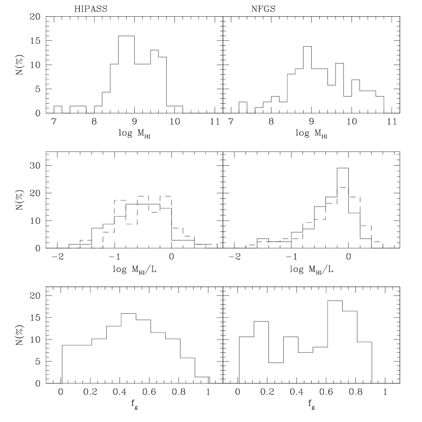
Figure 10: The properties concerning the gas content (Hi mass, $M_{HI}$, gas-to-light ratio, $M_{HI}/L$, and gas-mass-fraction, $f_{g}$) of the HiPASS sample along with similar histograms for the NFGS galaxies; the solid and dashed lines represent B-band and R-band data respectively; distance dependent quantities are computed with $h$=0.70.

The PEGASE models were also used in the calculation of the gas mass fractions for the galaxies. All of the models run produce values that follow a similar trend between B-R color and stellar mass-to-light ratio, $\Upsilon_{\ast}$. The trend is well approximated by log$(\Upsilon_{\ast_{B}})$=1.41(B-R)-1.55. The distributions of gas mass fractions for the samples are plotted in Fig. 10.

4.4 Surface Brightness and Number, Luminosity, and SFR Densities

The effect of any surface brightness bias on the measured value of the number, luminosity, and SFR densities can be explored by computing the values as functions of surface brightness for the HiPASS sample. All but four of the HiPASS galaxies have Hi masses that would make them detectable within HiPASS at or beyond our radial velocity limit of 2500 km s^-1 for $h$=0.70. Of these four, two are below the 3$\sigma$ detection limit of 40 mJy; the four galaxies have a wide range of surface brightness values. Therefore, we have taken the HiPASS sample to be volume limited for calculating the number, luminosity, and SFR densities as functions of surface brightness while including a correction factor of $\frac{132}{69}$ to account for the galaxies that met the selection criteria but were not imaged.

Given the somewhat complex selection criteria used for the NFGS, computing these densities as functions of $\mu_{e}$ for that sample would be difficult. The larger volume covered by the NFGS would also reduce the usefulness of any direct comparison of these quantities between the NFGS and the HiPASS sample. We therefore asses the degree to which the surface brightness bias may effect the measured number, luminosity, and SFR densities by exploiting the difference in the surface brightness coverage between these two samples. To do this, we compute the mean and standard deviation for the distributions for $\mu_{e}$ for both the entire NFGS and for the IRAS galaxies contained within the NFGS for which SFRs have been measured. The mean $\pm$2$\sigma$ for the the NFGS are displayed in Fig. 15 along with $\mu_{e}$ versus number and luminosity densities for the HiPASS sample; similar values for the NFGS/IRAS galaxies are displayed with the HiPASS sample values for $\mu_{e}$ versus SFR density. For the three $\mu_{e}$ bins that are more than 2$\sigma$ fainter than the mean for the NFGS, the total number and luminosity density was calculated and compared with the total values for all the bins. It was found that 14$\pm$5.0(1$\sigma$)% of the total number density is contained within these three bins. The bins contain a much smaller fraction of the total luminosity density; the value ranges from 0.5$\pm$0.2(1$\sigma$)% if the isophotal fluxes are used and 0.8$\pm$0.3(1$\sigma$)% if the total extrapolated fluxes are used. Four surface brightness bins are more than 2$\sigma$ fainter than the mean for the NFGS/IRAS galaxies. It was found that 3.9$\pm$1.6(1$\sigma$)% of the total SFR density is contained within these bins.

5 Conclusions

5.1 The Surface Brightness Bias

The existence of a bias toward higher surface brightness disks in flux limited optical catalogs is clearly illustrated by the comparison of properties of the HiPASS and NFGS samples. Nearly 25% of the galaxies in the HiPASS sample, which was chosen from the HiPASS catalog purely by declination and radial velocity, have half-light surface brightness values $\geq$24. Only about 3.6% of the optically selected NFGS galaxies have values that lie beyond this limit; this value increases slightly to 4.4% if only spiral galaxies are considered. The existence of this bias has been known and examined for quite some time (e. g. Disney, 1976; Impey & Bothun, 1997; Bothun, Impey, & McGaugh, 1997). However, the degree to which this bias effects our knowledge of the properties of the local galaxy population is largely dependent on the properties of interest.

5.2 The Galaxy Luminosity Function

Zwaan, Briggs, & Sprayberry (2001) have demonstrated that for a sample of galaxies similar to the HiPASS sample taken from the Arecibo Hi Strip Survey (AHiSS), the luminosity function is very similar to those found for optical samples. Other authors (e. g. Brown et al., 2001) have confirmed that the inclusion of LSB disks in optically selected samples changes the inferred luminosity function very little. Our results are in agreement with this conclusion as Fig. 15 implies that a sample biased toward higher surface brightness galaxies will miss less than 1% of the total local luminosity density.

However, it should be noted that Fig. 15 also indicates that the degree to which LSB galaxies contribute to the local galaxy LF depends greatly on how their luminosities are measured. Given that the central surface brightness values for these objects are quite low, it is easy to miss a significant portion of the light emitted by these objects. For example, for a galaxy with $\mu_{B,\circ}$=24, if the galaxy is approximated with a pure exponential disk, the total flux can be up to a factor of three times larger than the isophotal flux depending on the scale length of the disk. This is seen most prominently in the lowest surface brightness bin in the middle panel of Fig. 15; for this bin, the luminosity density calculated using the total extrapolated fluxes is about 30 times greater than that calculated using the isophotal luminosities.

5.3 Star Formation in the Local Universe

Fig. 15 indicates that LSB galaxies can contribute a small amount to the total local star formation that may be missed by optical surveys but that also appears to be overlooked by IR surveys such as the one performed by IRAS. This is mainly caused by the moderate sensitivity of the IRAS survey ($\sim$0.6 Jy at 60 $\mu$m (Saunders et al., 1995)), but still reflects the fact that the optimal wavelength regime in which to search for these objects is most likely the radio at rest frame 21 cm. Based on Fig. 15, the exclusion of these galaxies from samples selected in the optical (or IR) used to calculate the local SFR may miss up to 3 to 4% of the total amount of star formation.

It is also clear that the HiPASS sample contains a higher fraction of bluer galaxies that have high H$\alpha$ equivalent widths, indicating that the current star formation in these galaxies is fairly high when compared to how many stars have formed in them in the past. Fig. 13 and 14 demonstrate that the colors, equivalent widths, and SFRs per unit Hi mass are what is expected for stellar populations with young mean ages; Schmidt Law models estimate the typical mean age to be about 4.0 Gyr for Z=$\frac{1}{3}$Z_⊙. This is nearly 2 Gyr smaller than the median age estimated for the NFGS for solar metallicity, implying that on average, bluer more LSB galaxies that are present in lower numbers in the NFGS formed the majority of their stars more recently. The range in ages for the HiPASS sample is $\sim$1 Gyr smaller than that for the NFGS, implying that the majority of the star formation activity that has occurred in similar objects has taken place over a smaller range in redshift space. If it is assumed that the typical mean age for the HiPASS sample is about 4 Gyr with an rms deviation of 3.2 Gyr, then one would expect the progenitors of the blue LSB galaxies seen locally to contain few if any stars at redshifts of $\sim$1 or greater (i. e. look-back time greater than about 7.2 Gyr).

The authors would like to thank the NOAO TAC for allocation of observing time and the CTIO staff for expert assistance at the telescope as well as the referee for useful comments and suggestions.

Figure 1: The difference in the H$\alpha$ and R-band calibrations as a function of continuum subtraction scaling factor, $a$, and exposure times for all data calibrated with standard stars. The solid and dashed lines are the mean value for $C$ $\pm 2\sigma$ (see Sec. 2.2) used to compute the H$\alpha$ calibration from the R-band data for galaxies imaged during the final two nights of the second observing run (see Sec. 2.2 for a more detailed discussion). The two discrete larger groups of points correspond to the two different types of H$\alpha$ filters used, the 30 Å Rand filters (lower group) and 75 Å CTIO filters (upper group). Within each larger group, there are two smaller discrete groups; for the Rand filters, the upper group corresponds to the 657 nm filter and the lower group corresponds to the 660 and 661 nm filters; for the CTIO filters, the upper group corresponds to the calibration for the first observing run and the lower group corresponds to the calibration for the second run.

Figure 2: Comparison of the photometry performed on the HiPASS sample and that found in the literature (see Sec. 3.1 and 3.2 for references) for B-band magnitudes (upper left), apparent (B-R) color indexes (upper right), H$\alpha$ fluxes corrected for extinction and $[$NII$]$ contamination (lower left), and H$\alpha+[$NII$]$ fluxes (lower right). The open circles are data derived from questionable calibration (see Sec. 2.2); the open box is M83; the error bars represent the 1$\sigma$ errors in the photometry. In the lower right panel, the point that deviates from the published value by 0.85 dex is discussed in Sec. 3.2.

Figure 4: Example surface brightness profiles for 6 disk morphologies along with the exponential fits; the lower points are the B-band profiles; the upper points are the R-band profiles; all values of $\mu$ are corrected for Galactic extinction; all radii are in units of arcseconds. The horizontal dashed lines represent the B-band 1$\sigma$ limiting isophote (corrected for Galactic extinction).

Figure 5: The distribution of morphological types among the 132 HiPASS galaxies initially selected (top panel), HiPASS galaxies included in this study (middle panel), and the NFGS galaxies (bottom panel).

Figure 6: B-R color derived from the exponential disk parameters versus the B-R color within the effective radius for the HiPASS and NFGS galaxies. NFGS galaxies are represented by $\times$’s; closed boxes represent HiPASS galaxies; open circles represent HiPASS galaxies for which the calibration is questionable; the open box is M83. All colors are corrected for Galactic reddening. The displayed error bars are the median 1$\sigma$ errors for the HiPASS galaxies. The line plotted is what would be expected if the disk and effective radius colors were the same; the points do not follow this trend as the majority of the points for both samples have disk colors that are bluer than their effective radius colors.

Figure 7: Disk scale length versus effective radius (upper panel) and central disk surface brightness versus surface brightness at the effective radius (lower panel). NFGS galaxies are represented by $\times$’s; closed boxes represent HiPASS galaxies; open circles represent HiPASS galaxies for which the calibration is questionable; the open box is M83. The displayed error bars are the median 1$\sigma$ errors for the HiPASS galaxies. The lines in both panels represent the relations expected for pure exponential disks; the HiPASS galaxies follow these trends well whereas the NFGS galaxies do not.

Figure 8: The properties of the HiPASS sample pertaining to the distribution of stellar light (surface brightness at the half-light radius, $\mu_{e}$, central disk surface brightness, $\mu_{o}$, half-light radius, $r_{e}$, and disk scale length, $h$) along with similar histograms for the NFGS galaxies; the solid and dashed lines represent B-band (effective radius) and R-band (disk scale length) data respectively; distance dependent quantities are computed with $h$=0.70.

Figure 9: The properties concerning the stellar content (color at the effective radius, (B-R)_e, total extrapolated absolute magnitude, $M_{T}$, and star formation rate, SFR) of the HiPASS sample along with similar histograms for the NFGS galaxies; the solid and dashed lines represent B-band and R-band data respectively; distance dependent quantities are computed with $h$=0.70.

Figure 11: Ellipticity (e=1-$\frac{b}{a}$) versus (B-R)_e color. NFGS galaxies are represented by $\times$’s; closed boxes represent HiPASS galaxies; open circles represent HiPASS galaxies for which the calibration is questionable; the open box is M83. The mean values for (B-R)_e for bins in ellipticity are plotted with the data; stars represent the NFGS galaxies; closed circles represent the HiPASS galaxies.

Figure 12: The R-band gas-to-light ratio as a function of surface brightness at the effective radius and absolute magnitude. The solid lines are linear least-squares fits to the data. NFGS galaxies are represented by $\times$’s; closed boxes represent HiPASS galaxies; open circles represent HiPASS galaxies for which the calibration is questionable; the open box is M83. The displayed error bars are the median 1$\sigma$ errors for the HiPASS galaxies.

Figure 13: Reddening corrected, total extrapolated (B-R)_T color versus H$\alpha$ equivalent width with model predictions based on different star formation histories. Here, $\Psi_{\circ}$ refers to the initial SFR in units of M_gal Myr^-1 where M_gal is the combined mass of stars and gas; $\tau$ refers to the e-folding time for the exponential models (i. e. $\tau\Psi_{\circ}$ gives the total amount of mas formed at t$\rightarrow\infty$). See Sec. 4.3 for a detailed discussion of the model curves plotted. NFGS galaxies are represented by $\times$’s; closed boxes represent HiPASS galaxies; open circles represent HiPASS galaxies for which the calibration is questionable; the open box is M83. The displayed error bars are the median 1$\sigma$ errors for the HiPASS galaxies.

Figure 14: Reddening corrected (B-R)_T color versus SFR per unit HI mass. The lines are generated by the same models as the ones plotted in Fig. 13. NFGS galaxies are represented by $\times$’s; closed boxes represent HiPASS galaxies; open circles represent HiPASS galaxies for which the calibration is questionable; the open box is M83. The displayed error bars are the median 1$\sigma$ errors for the HiPASS galaxies.

Figure 15: Half-light surface brightness versus number (top panel), luminosity (middle panel), and SFR (bottom panel) densities for the HiPASS sample; the vertical error bars are 1$\sigma$ error bars; the horizontal bars represent the width of the surface brightness bins. The $\times$’s in the middle panel represent values calculated with isophotal fluxes; the boxes represent values calculated with total extrapolated fluxes. The solid vertical lines in the top and middle panels represent the mean value for $\mu_{e}$ for the NFGS galaxies; the dashed lines represent the mean $\pm 2\sigma$; the lines in the lower panel represent the same quantities for the NFGS/IRAS galaxies.

Table 1: Observations

Galaxy	UT Date	RA	DEC	$\tau_{B}$	$\tau_{R}$	$\tau_{H\alpha}$	H$\alpha$ Filter
		(2000.0)	(2000.0)	(s)	(s)	(s)
CTIO March 2-9, 2000
NGC1313	000303	03 18 16.48	-66 30 33.8	2$\times$300	2$\times$300	2$\times$1200	657 nm
ESO004-G017	000303	05 04 29.36	-87 01 45.0	2$\times$300	2$\times$300	2$\times$1200	660 nm
ESO035-G020	000303	08 03 18.61	-77 04 18.7	2$\times$300	2$\times$300	2$\times$1200	660 nm
HIPASS1039-71	000303	10 39 40.00	-71 55 23.0	2$\times$300	2$\times$300	2$\times$1200	660 nm
ESO092-G006	000303	10 03 18.96	-64 58 03.9	2$\times$300	2$\times$300	2$\times$1200	661 nm
IC4662	000303	17 47 06.38	-64 38 25.1	2$\times$300	2$\times$300	2$\times$1200	657 nm
ESO084-G040	000304	04 44 59.88	-62 42 24.5	2$\times$300	2$\times$300	2$\times$1200	660 nm
ESO059-G001	000304	07 31 18.20	-68 11 16.8	2$\times$300	2$\times$300	2$\times$1200	657 nm
ESO060-G019	000304	08 57 26.20	-69 03 35.9	2$\times$300	2$\times$300	2$\times$1200	660 nm
ESO091-G007	000304	09 17 30.88	-62 53 03.3	2$\times$300	2$\times$300	2$\times$1200	661 nm
ESO092-G021	000304	10 21 05.37	-66 29 27.2	2$\times$300	2$\times$300	2$\times$1200	661 nm
NGC6438A	000304	18 22 43.24	-85 24 14.6	2$\times$300	2$\times$300	2$\times$1200	661 nm
ESO086-G060	000305	06 08 09.26	-63 35 16.8	2$\times$300	2$\times$300	2$\times$1200	660 nm
ESO036-G006	000305	08 38 47.09	-75 09 23.4	2$\times$300	2$\times$300	2$\times$1200	6600 Å
NGC2397A	000305	07 21 07.82	-69 06 59.7	2$\times$300	2$\times$300	2$\times$1200	660 nm
NGC2915	000305	09 26 11.49	-76 37 35.6	2$\times$300	2$\times$300	2$\times$1200	657 nm
IC3104	000305	12 18 46.06	-79 43 33.8	2$\times$300	2$\times$300	2$\times$1200	657 nm
ESO021-G003	000305	13 32 27.28	-80 25 56.5	2$\times$300	2$\times$300	2$\times$1200	661 nm
ESO085-G014	000306	04 54 42.75	-62 47 59.1	2$\times$300	2$\times$300	2$\times$1200	660 nm
NGC1892	000306	05 17 07.98	-64 57 41.0	2$\times$300	2$\times$300	2$\times$1200	660 nm
NGC2836	000306	09 13 44.60	-69 20 05.1	2$\times$300	2$\times$300	2$\times$1200	660 nm
ESO035-G021	000306	08 09 55.49	-74 30 41.8	2$\times$300	2$\times$300	2$\times$1200	660 nm
ESO019-G004	000306	10 48 50.14	-80 14 12.4	2$\times$300	2$\times$300	2$\times$1200	660 nm
NGC6300	000306	17 16 59.22	-62 49 11.2	2$\times$300	2$\times$300	2$\times$1200	6600 Å
ESO085-G047	000307	05 07 43.86	-62 59 24.3	2$\times$300	2$\times$300	2$\times$1200	660 nm
ESO037-G004	000307	09 32 37.51	-74 15 16.0	2$\times$300	2$\times$300	2$\times$1200	660 nm
ESO090-G004	000307	08 38 36.86	-64 20 32.4	2$\times$300	2$\times$300	2$\times$1200	660 nm
ESO061-G017	000307	09 52 33.70	-69 04 04.2	2$\times$300	2$\times$300	2$\times$1200	660 nm
NGC3136A	000307	10 03 33.49	-67 26 52.5	2$\times$300	2$\times$300	2$\times$1200	661 nm
ESO038-G011	000307	11 20 58.10	-75 52 45.4	2$\times$300	2$\times$300	2$\times$1200	660 nm
ESO140-G019	000307	18 22 46.46	-62 16 12.8	2$\times$300	2$\times$300	2$\times$1200	657 nm
HIPASS0635-70	000308	06 35 36.00	-70 52 55.0	2$\times$300	2$\times$300	2$\times$1200	660 nm
NGC2442	000308	07 36 23.77	-69 31 49.5	2$\times$300	2$\times$300	2$\times$1200	660 nm
NGC2788B	000308	09 03 37.19	-67 57 58.9	2$\times$300	2$\times$300	2$\times$1200	660 nm
ESO060-G007	000308	08 27 26.50	-71 04 19.3	2$\times$300	2$\times$300	2$\times$1200	660 nm
ESO037-G015	000308	10 25 41.99	-76 30 18.3	2$\times$300	2$\times$300	2$\times$1200	660 nm
NGC5068	000308	13 18 55.24	-21 02 21.5	2$\times$300	2$\times$300	2$\times$1200	657 nm
IC4710	000308	18 28 38.16	-66 58 54.3	2$\times$300	2$\times$300	2$\times$1200	657 nm
HIPASS0653-73	000309	06 53 50.00	-73 40 35.0	2$\times$300	2$\times$300	2$\times$1200	6600 Å
ESO060-IG003	000309	08 16 33.69	-71 51 35.0	2$\times$300	2$\times$300	2$\times$1200	660 nm
NGC3059	000309	09 50 07.95	-73 55 17.3	2$\times$300	2$\times$300	2$\times$1200	6600 Å
ESO037-G010	000309	10 04 16.71	-75 28 43.0	2$\times$300	2$\times$300	2$\times$1200	660 nm
M83	000309	13 37 00.23	-29 52 04.5	2$\times$300	2$\times$300	2$\times$1200	657 nm
ESO104-G022	000309	18 55 41.24	-64 48 39.2	2$\times$300	2$\times$300	2$\times$1200	657 nm
CTIO October 23-28, 2000
NGC7098	001025	21 44 16.49	-75 06 44.3	2$\times$480	2$\times$300	2$\times$1800	6600 Å
NGC0802	001025	01 59 06.98	-67 52 10.4	2$\times$480	2$\times$300	2$\times$1800	6600 Å
ESO054-G021	001025	03 49 50.18	-71 38 07.1	2$\times$420	2$\times$300	2$\times$1800	6600 Å
IC2051	001025	03 52 02.29	-83 49 56.6	2$\times$420	2$\times$300	2$\times$1800	6600 Å
ESO027-G001	001026	21 52 27.81	-81 31 50.5	2$\times$480	2$\times$300	2$\times$1800	6600 Å
ESO013-G016	001026	01 32 48.37	-79 28 26.4	2$\times$480	2$\times$300	2$\times$1800	6600 Å
NGC1511	001026	03 59 35.73	-67 38 06.6	2$\times$420	2$\times$300	2$\times$1800	6600 Å
ESO119-G016	001026	04 51 29.19	-61 39 03.4	2$\times$480	2$\times$300	2$\times$1800	6563 Å
ESO027-G021	001027	23 04 19.50	-79 28 01.1	2$\times$420	2$\times$300	2$\times$1800	6600 Å
NGC0406	001027	01 07 24.12	-69 52 35.3	2$\times$420	2$\times$300	2$\times$1800	6600 Å
NGC1559	001027	04 17 37.29	-62 47 03.6	2$\times$420	2$\times$300	2$\times$1800	6600 Å
ESO085-G030	001027	05 01 30.02	-63 17 33.9	2$\times$420	2$\times$300	2$\times$1800	6600 Å
NGC1809	001027	05 02 05.63	-69 34 07.9	2$\times$480	2$\times$300	2$\times$1200	6600 Å
IC4870	001028	19 37 38.25	-65 48 45.3	2$\times$420	2$\times$300	2$\times$1800	6600 Å
NGC7661	001028	23 27 14.51	-65 16 12.6	2$\times$480	2$\times$300	2$\times$1800	6600 Å
NGC2082	001028	05 41 50.51	-64 18 00.9	2$\times$480	2$\times$300	2$\times$1800	6600 Å
ESO017-G002	001028	07 32 20.37	-77 55 07.5	2$\times$420	2$\times$300	2$\times$1800	6600 Å
ESO035-G009	001028	07 28 40.95	-75 03 14.9	2$\times$600	2$\times$600	$\cdots$	$\cdots$
CTIO November 2, 5, & 6, 2000
IC5028	001102	20 43 21.86	-65 38 47.7	2$\times$600	2$\times$420	2$\times$1200	660 nm
ESO079-G005	001102	00 40 43.53	-63 26 30.7	2$\times$480	2$\times$300	2$\times$1200	660 nm
ESO080-G006	001102	01 47 16.94	-62 58 13.3	2$\times$480	2$\times$300	2$\times$1200	660 nm
ESO035-G018	001102	07 55 03.97	-76 24 41.3	2$\times$480	2$\times$300	2$\times$1200	660 nm
IC2554	001102	10 08 51.24	-67 01 39.5	2$\times$420	$\cdots$	$\cdots$	$\cdots$
IC5176	001106	22 14 52.33	-66 51 31.7	2$\times$480	2$\times$300	2$\times$1800	660 nm
ESO079-G007	001106	00 50 03.84	-66 33 09.3	2$\times$480	2$\times$300	2$\times$1800	660 nm
ESO035-G009	001106	07 28 40.95	-75 03 14.9	2$\times$600	2$\times$600	2$\times$1200	659 nm
IC2554	001106	10 08 51.24	-67 01 39.5	2$\times$420	2$\times$300	2$\times$1200	659 nm

Table 2: Standard Star Fields

Observing run	Photometric Standards	Spectrophotmetric Standards
CTIO, March 2-9, 2000	PG1525-071	LTT 4364
	PG1525-071A	LTT 1788
	PG1525-071B	LTT 6248
	PG1525-071C
	PG1525-071D
CTIO, Oct. 23-28, Nov. 2, 5, 6, 2000	PG0231+051	LTT 1020
	PG0231+051A	LTT 377
	PG0231+051B
	PG0231+051C
	PG0231+051D
	PG0231+051E
	GD 50

Table 3: Photometric Calibration Coefficients

Observing run	Filter	k	t	z
CTIO, March 2-9, 2000	B	0.28$\pm$0.031	0.090$\pm$0.010	1.80$\pm$0.041
	R	0.13$\pm$0.018	0.050$\pm$0.0058	1.64$\pm$0.024
	657 nm	0.069$\pm$0.10	$\cdots$	5.48$\pm$0.13
	660 nm	0.072$\pm$0.087	$\cdots$	5.64$\pm$0.11
	661 nm	0.070$\pm$0.079	$\cdots$	5.68$\pm$0.10
	6600 Å	0.135$\pm$0.093	$\cdots$	4.65$\pm$0.12
CTIO, Oct. 23-28, 2000	B	0.25$\pm$0.010	0.061$\pm$0.0044	1.69$\pm$0.014
	R	0.10$\pm$0.039	-0.015$\pm$0.011	1.58$\pm$0.053
	6563 Å	0.071$\pm$0.051	$\cdots$	4.64$\pm$0.061
	6600 Å	0.067$\pm$0.024	$\cdots$	4.67$\pm$0.029
CTIO, Nov. 2, 2000	B	0.27$\pm$0.013	0.069$\pm$0.0034	1.68$\pm$0.018
	R	0.10$\pm$0.0079	-0.0024$\pm$0.0025	1.59$\pm$0.011

Table 4: Isohpotal Data

Galaxy	Type	r25	m${}_{B_{25}}$	m${}_{R_{25}}$	E(B-V)	$i$	PA
		(′′)				(∘)	(∘)
ESO004-G017	Sm	23	16.1	15.4	0.137	58	54
ESO013-G016	Sc	51	13.5	12.5	0.072	48	-11
ESO017-G002	S0	27	14.6	13.0	0.248	18	-5
ESO019-G004	Sd	19	15.4	14.3	0.125	70	31
ESO021-G003	Sbc	39	13.8	12.6	0.242	51	60
ESO027-G001	Sc	62	13.0	9.4	0.199	42	-43
ESO027-G021	Sa	27	14.2	13.0	0.103	10	-90
ESO035-G009$\ast$${\dagger}$	Sm	19	17.6	16.9	0.207	74	21
ESO035-G018$\ast$	Sc	49	13.5	13.4	0.180	75	-42
ESO035-G020	Sm	25	15.7	14.9	0.114	47	30
ESO035-G021	Sm	19	16.3	14.9	0.183	69	128
ESO036-G006	Sd	45	14.1	13.1	0.129	62	-18
ESO037-G004	Sm	12	17.2	16.1	0.111	28	-10
ESO037-G010	Sc	65	13.1	11.8	0.385	33	-16
ESO037-G015$\ast$	Sdm	15	16.9	15.3	0.404	67	-67
ESO038-G011	Sb	18	16.2	14.8	0.305	63	41
ESO054-G021	Scd	90	12.7	13.1	0.051	61	-90
ESO059-G001	Sm	51	14.2	13.1	0.146	31	-36
ESO060-G007$\ast$	Scd	12	16.3	14.8	0.187	75	34
ESO060-G019	Sc	67	12.1	11.3	0.100	61	-19
ESO060-IG003	Irr	18	15.2	14.1	0.136	28	-6
ESO061-G017	Sd	25	15.2	14.0	0.174	62	-54
ESO079-G005$\ast$	Scd	42	13.9	11.0	0.020	59	-5
ESO079-G007$\ast$	Sc	42	13.7	12.8	0.017	31	5
ESO080-G005$\ast$	Sm	32	13.8	13.0	0.026	56	65
ESO084-G040	Sm	28	15.1	14.4	0.035	46	57
ESO085-G014	Sm	60	13.1	12.3	0.035	67	86
ESO085-G030	Irr	31	13.9	12.9	0.030	63	-28
ESO085-G047	Irr	32	15.1	14.3	0.025	53	29
ESO086-G060	Irr	20	16.1	15.3	0.050	53	-63
ESO090-G004	IBm	31	15.1	14.0	0.157	42	-88
ESO091-G007	Im	44	13.6	12.5	0.193	60	-4
ESO092-G006	Sb	47	13.1	11.8	0.227	55	35
ESO092-G021	Irr	44	13.2	11.9	0.238	49	61
ESO104-G022	Im	29	15.3	14.1	0.084	51	-72
ESO119-G016	Sm	39	15.0	14.1	0.025	66	25
ESO140-G019	Irr	18	16.6	15.9	0.080	47	34
HIPASS0635-70$\ast$	Sc	12	17.7	16.7	0.069	46	-90
HIPASS0653-73	Sd	12	17.9	16.8	0.133	62	-40
HIPASS1039-71	Irr	9	17.8	16.5	0.149	33	-72
IC2150	Sc	64	12.2	10.9	0.113	53	73
IC2554$\ast$	merger	33	14.7	13.4	0.204	65	4
IC3104	Sm	68	12.9	11.5	0.407	60	36
IC4662	Im	81	11.2	10.4	0.070	48	-77
IC4710$\ast$	Sm	80	12.9	11.7	0.089	15	-62
IC4870	Im	38	13.9	15.0	0.113	58	-42
IC5028$\ast$	Sm	28	15.6	14.9	0.048	53	-11
IC5176$\ast$	Sbc	54	13.2	11.8	0.031	80	29
M83	Sab	279	8.5	7.5	0.066	13	85
NGC0406	Sc	59	12.9	12.0	0.023	65	-19
NGC0802	Sa	24	14.2	21.4	0.024	43	-20
NGC1313	Sc	219	10.0	9.2	0.102	37	1
NGC1511	Sc	68	12.0	10.9	0.061	68	-55
NGC1559	Scd	90	10.9	10.0	0.030	53	65
NGC1809	Scd	68	12.2	11.0	0.221	69	-37
NGC1892	Sc	51	12.8	11.7	0.084	71	75
NGC2082	Sc	51	12.7	11.6	0.058	24	51
NGC2397B	Irr	24	15.2	14.1	0.200	60	86
NGC2442$\ast$	Sbc	130	11.6	10.0	0.203	21	-67
NGC2788B$\ast$	Sab	27	14.9	13.7	0.111	64	-17
NGC2836	Sbc	53	13.1	11.9	0.093	56	-69
NGC2915	Irr	51	13.2	12.0	0.276	57	-53
NGC3059	Sc	98	11.9	10.6	0.244	21	57
NGC3136A	Im	27	15.2	13.9	0.216	75	84
NGC5068$\ast$	SBd	180	10.7	9.7	0.102	24	-76
NGC6300	Sb	126	10.5	9.2	0.097	48	-65
NGC6438A	Ring	54	12.6	11.5	0.170	60	29
NGC7098	Sa	91	12.4	11.1	0.087	51	70
NGC7661	Sc	42	14.2	13.3	0.026	47	30

Note. — The images for any galaxy with a $\ast$ by its name were most likely taken through clouds (the same notation is used in Tables 5 and 6) and the values listed should be taken as estimates only. For galaxies marked by a ${\dagger}$, the data are for the 26 mag. arcsec.^-2 isophote.

Table 5: Surface Brightness Profile Data

Galaxy	BT	RT	(B-R)e	re	$\mu_{e,B}$	$\mu_{e,R}$	$h$	$\mu_{o,B}$	$\mu_{o,R}$
				(′′)	(mag/$\Box^{\prime\prime}$)	(mag/$\Box^{\prime\prime}$)	(′′)	(mag/$\Box^{\prime\prime}$)	(mag/$\Box^{\prime\prime}$)
ESO004-G017	14.5	13.9	0.56	31.1	24.7	24.1	19.4	22.9	22.4
ESO013-G016	13.0	12.2	0.86	25.9	22.8	21.9	11.0	19.7	18.8
ESO017-G002	13.3	12.2	1.13	9.3	21.1	20.1	9.1	20.6	19.5
ESO019-G004	14.8	13.9	0.80	12.4	23.1	22.4	5.5	20.7	19.9
ESO021-G003	12.6	11.8	0.82	22.2	22.4	21.7	11.5	20.3	19.5
ESO027-G001	11.8	10.9	0.99	37.0	22.4	21.6	13.2	18.6	17.9
ESO027-G021	13.7	12.7	1.03	7.1	21.0	19.9	6.6	20.0	19.2
ESO035-G009$\ast$	15.7	13.7	1.99	24.2	25.6	23.7	18.4	24.1	22.2
ESO035-G018$\ast$	12.6	11.6	1.06	21.8	22.4	21.5	14.3	20.6	19.9
ESO035-G020	14.4	13.6	0.72	25.2	24.4	23.9	16.4	22.8	22.1
ESO035-G021	12.3	12.0	0.41	25.4	24.3	23.9	25.9	23.3	22.8
ESO036-G006	13.1	12.3	0.72	35.5	24.1	23.2	23.9	22.4	21.6
ESO037-G004	14.0	13.3	0.67	65.2	25.8	25.2	40.5	24.1	23.4
ESO037-G010	11.0	10.4	0.59	36.1	22.1	21.3	32.8	21.1	20.3
ESO037-G015$\ast$	14.4	13.6	0.95	15.8	23.1	22.6	10.6	21.7	21.0
ESO038-G011	13.9	12.7	1.04	15.0	23.0	22.3	7.1	20.8	20.1
ESO054-G021	12.2	11.3	0.85	54.8	23.6	22.8	31.0	21.6	20.8
ESO059-G001	12.6	11.9	0.80	52.8	24.3	23.7	27.2	22.3	21.6
ESO060-G007$\ast$	15.5	14.5	1.16	13.7	24.3	23.5	11.0	23.0	22.1
ESO060-G019	11.6	10.9	0.63	34.8	22.9	22.1	19.0	20.6	20.0
ESO060-IG003	14.5	13.6	0.70	6.7	21.9	21.1	4.9	20.4	19.4
ESO061-G017	14.3	13.3	0.93	16.0	23.0	22.1	8.9	21.1	20.2
ESO079-G005$\ast$	13.7	12.8	0.92	20.8	23.0	22.2	12.3	21.2	20.4
ESO079-G007$\ast$	13.5	12.6	0.83	20.8	22.8	22.0	12.1	20.9	19.9
ESO080-G005$\ast$	13.6	12.8	0.84	18.0	23.1	22.4	8.6	20.7	20.0
ESO084-G040	14.7	14.1	0.64	15.3	23.5	22.9	9.6	21.7	21.2
ESO085-G014	12.8	12.1	0.73	30.7	23.0	22.3	14.9	20.5	19.9
ESO085-G030	13.7	12.8	0.93	9.2	21.2	20.4	7.1	20.3	19.4
ESO085-G047	13.9	13.2	0.77	45.8	25.2	24.6	31.9	23.4	22.7
ESO086-G060	15.6	15.0	0.65	13.2	24.0	23.4	8.0	22.2	21.7
ESO090-G004	14.0	13.2	0.74	21.0	23.3	22.6	13.2	21.7	21.1
ESO091-G007	12.6	11.9	0.77	24.6	22.4	21.8	12.5	20.3	19.6
ESO092-G006	10.9	10.6	0.64	48.3	23.9	23.4	13.4	19.9	19.4
ESO092-G021	11.4	10.6	0.92	42.1	23.6	23.0	33.6	22.0	21.4
ESO104-G022	13.7	12.8	1.03	46.0	25.1	24.3	35.9	23.7	22.9
ESO119-G016	14.2	13.5	0.77	35.6	24.7	24.0	21.9	23.0	22.3
ESO140-G019	15.2	14.6	0.56	22.9	24.8	24.2	14.9	23.1	22.6
HIPASS0635-70$\ast$	16.7	15.8	0.92	11.2	24.6	23.9	7.0	23.0	22.0
HIPASS0653-73	16.1	15.2	0.82	17.6	25.0	24.2	10.9	23.3	22.5
HIPASS1039-71	16.9	15.8	1.16	7.2	24.0	23.2	4.2	22.2	21.3
IC2150	11.7	10.6	1.27	30.8	21.7	20.7	10.5	17.8	16.7
IC2554$\ast$	13.8	12.8	1.08	19.2	22.9	22.0	11.0	21.1	20.2
IC3104	10.8	10.1	0.55	31.1	21.7	20.9	28.6	20.6	19.7
IC4662	10.8	10.0	0.62	37.3	22.1	21.3	21.7	20.5	19.5
IC4710$\ast$	12.1	11.1	1.07	60.3	23.6	22.9	40.2	22.3	21.5
IC4870	13.1	14.4	-1.15	20.8	23.0	24.7	13.2	21.3	22.9
IC5028$\ast$	14.9	14.3	0.72	21.2	24.2	23.6	12.8	22.5	21.9
IC5176$\ast$	13.0	11.7	1.50	23.0	22.7	21.5	13.9	20.7	19.7
M83	8.2	7.3	1.06	126.8	21.4	20.5	21.9	10.8	9.7
NGC0406	12.7	11.8	0.95	25.3	22.6	21.7	19.3	21.5	20.6
NGC0802	14.0	13.2	0.67	5.5	20.7	19.9	8.1	21.6	20.6
NGC1313	9.5	8.8	0.63	94.6	22.5	21.7	59.3	20.6	19.9
NGC1511	11.7	10.6	0.99	20.9	21.2	20.1	17.7	20.6	19.4
NGC1559	10.7	9.8	0.85	33.0	21.0	20.1	18.9	19.6	18.7
NGC1809	10.7	9.9	0.76	60.5	23.2	22.8	30.0	21.2	20.8
NGC1892	12.3	11.4	0.90	21.8	21.7	20.9	10.3	19.3	18.4
NGC2082	12.4	11.4	1.03	22.0	21.5	20.6	10.7	19.7	18.5
NGC2397B	14.2	13.3	0.80	14.6	22.9	22.1	9.1	21.2	20.3
NGC2442$\ast$	10.3	9.1	1.29	104.3	23.2	22.1	65.9	21.6	20.5
NGC2788B$\ast$	14.3	13.2	0.90	13.7	22.8	21.8	9.6	21.6	20.3
NGC2836	12.5	11.4	1.09	26.8	22.7	21.6	16.6	21.0	19.9
NGC2915	11.7	11.0	0.58	18.7	21.3	20.4	17.5	20.6	19.7
NGC3059	10.2	9.5	0.88	74.4	23.0	22.2	38.7	20.9	20.2
NGC3136A	14.1	13.3	0.79	19.9	23.5	22.7	11.9	21.7	20.9
NGC5068$\ast$	10.1	9.3	0.94	97.8	22.8	22.0	46.1	20.3	19.5
NGC6300	10.0	8.8	1.12	56.2	21.6	20.5	31.6	20.1	18.8
NGC6438A	10.7	9.9	0.89	59.0	23.9	23.3	65.0	22.7	22.1
NGC7098	11.6	10.2	1.49	71.6	24.2	23.0	62.2	23.0	21.8
NGC7661	13.9	13.1	0.98	24.1	23.4	22.6	7.3	18.7	17.9

Note. — All colors and central surface brightnesses were corrected for Galactic extinction using E(B-V) values quoted in the NASA/IPAC Extragalactic Database (NED) and E(B-V) to A_ν conversion factors provided by Schlegel et al. (1998).

Table 6: Emission Line Data

Galaxy	log $F_{H\alpha+[NII]}$	log $F_{H\alpha}$	$W_{H\alpha+[NII]}$	$W_{H\alpha}$	$S_{HI}$	$\frac{M_{HI}}{L_{B}}$	$\frac{M_{HI}}{L_{R}}$	$V_{R}$	$V_{LG}$
	(ergs/s/cm2)	(ergs/s/cm2)	(Å)	(Å)	(Jy km/s)	(M⊙/L⊙)	(M⊙/L⊙)	(km/s)	(km/s)
ESO004-G017	-13.23	-12.92	30.2	29.2	4.2	0.39	0.70	1754	1750
ESO013-G016$\star$	-12.13	-11.83	21.4	18.0	2.3	0.06	0.08	1753	1737
ESO017-G002$\star$	-12.72	-12.26	8.9	7.5	4.9	0.16	0.17	1620	1607
ESO019-G004	-13.11	-12.79	14.5	14.4	2.3	0.28	0.38	2005	2013
ESO021-G003	-12.02	-11.41	14.1	13.4	5.5	0.10	0.14	2283	2287
ESO027-G001$\star$	-10.10	-9.43	131.8	111.9	29.1	0.24	0.30	2548	2543
ESO027-G021$\star$	-12.34	-11.96	21.4	19.1	10.2	0.47	0.55	2443	2433
ESO035-G009$\ast$$\star$	$\cdots$	$\cdots$	$\cdots$	$\cdots$	5.2	1.49	0.71	1122	1096
ESO035-G018$\ast$$\star$	-12.63	-12.13	14.5	13.6	15.6	0.25	0.32	1750	1745
ESO035-G020	-12.46	-12.13	112.2	107.6	10.8	0.91	1.37	1742	2211
ESO035-G021	-13.07	-12.73	26.3	20.8	3.8	0.05	0.11	1235	1215
ESO036-G006	-12.50	-12.21	20.9	17.9	24.0	0.64	0.89	1132	1112
ESO037-G004	-13.45	-13.22	37.2	32.0	4.0	0.24	0.39	1274	1263
ESO037-G010	-11.91	-11.06	21.4	19.6	16.5	0.07	0.11	1773	1781
ESO037-G015$\ast$	-13.23	-12.66	30.9	29.1	3.9	0.35	0.50	1610	1612
ESO038-G011	-13.20	-12.64	20.0	19.4	4.5	0.25	0.26	1879	1887
ESO054-G021$\star$	-12.07	-11.78	60.3	48.6	38.8	0.44	0.61	1425	1379
ESO059-G001	-12.48	-12.19	20.4	20.1	14.2	0.24	0.36	530	448
ESO060-G007$\ast$	-13.49	-13.19	10.2	9.6	0.1	0.03	0.03	1506	1502
ESO060-G019	-11.66	-11.27	21.4	17.3	44.4	0.28	0.47	1429	1428
ESO060-IG003	-12.94	-12.67	17.8	16.1	2.5	0.24	0.33	1415	1401
ESO061-G017	-13.10	-12.72	9.1	8.8	5.4	0.43	0.52	1748	1765
ESO079-G005$\ast$$\star$	-10.50	-10.26	263.0	250.0	21.1	0.97	1.31	1701	1687
ESO079-G007$\ast$$\star$	-12.13	-11.91	34.7	30.5	7.3	0.28	0.35	1476	1629
ESO080-G005$\ast$$\star$	-12.42	-12.21	20.0	18.2	7.9	0.35	0.49	1549	1486
ESO084-G040	-13.11	-12.99	13.5	11.9	0.5	0.06	0.10	1236	1163
ESO085-G014	-11.79	-11.56	45.7	39.2	21.0	0.42	0.67	1401	1327
ESO085-G030$\star$	-12.09	-11.91	34.7	30.3	15.7	0.72	0.93	1289	1223
ESO085-G047	-12.81	-12.63	25.1	22.7	9.8	0.55	0.82	1458	1385
ESO086-G060	-13.39	-13.22	18.6	18.0	3.9	1.06	1.82	1636	1585
ESO090-G004	-12.57	-12.17	38.0	37.2	4.1	0.25	0.37	1924	2083
ESO091-G007	-12.49	-11.96	3.3	3.0	6.4	0.11	0.16	2130	2174
ESO092-G006	-11.80	-11.15	12.0	10.9	15.0	0.05	0.12	2166	1739
ESO092-G021	-12.11	-11.45	7.4	6.1	28.3	0.16	0.22	2008	2040
ESO104-G022	-13.00	-12.75	17.0	17.0	15.2	0.70	0.88	794	804
ESO119-G016$\star$	-12.64	-12.48	32.4	31.7	11.5	0.87	1.29	961	882
ESO140-G019	-12.80	-12.61	134.9	134.9	4.1	0.73	1.32	959	975
HIPASS0635-70$\ast$	-14.50	-14.34	3.0	2.9	4.3	3.06	3.96	1611	1582
HIPASS0653-73	-14.03	-13.82	14.8	13.8	3.9	1.59	2.25	1202	1171
HIPASS1039-71	-14.70	-14.46	2.9	2.8	2.4	2.06	2.24	1537	1539
IC2150$\star$	-11.35	-10.89	31.6	24.2	17.4	0.13	0.13	1724	1709
IC2554$\ast$$\star$	-12.20	-11.79	60.3	58.6	14.0	0.74	0.88	1386	1388
IC3104	-12.29	-11.67	7.6	7.3	6.5	0.02	0.03	432	415
IC4662	-10.85	-10.58	70.8	67.3	99.0	0.31	0.46	304	391
IC4710$\ast$	-11.82	-11.49	33.1	33.0	25.9	0.27	0.31	737	744
IC4870$\star$	-12.22	-12.03	12.0	11.1	18.8	0.50	5.04	876	884
IC5028$\ast$$\star$	-12.82	-12.63	49.0	46.7	4.8	0.70	1.12	1620	1652
IC5176$\ast$$\star$	-12.12	-11.77	13.2	12.3	42.1	0.98	0.90	1723	1745
M83	-10.01	-9.27	35.5	32.8	417.3	0.12	0.15	516	751
NGC0406$\star$	-11.66	-11.41	46.8	38.5	34.4	0.61	0.79	1504	1473
NGC0802$\star$	-13.65	-13.48	1621.8	1422.3	2.5	0.15	0.21	1477	1428
NGC1313	-10.59	-10.21	34.7	33.3	219.5	0.21	0.34	457	350
NGC1511$\star$	-11.17	-10.83	46.8	36.4	59.9	0.42	0.48	1330	1271
NGC1559$\star$	-10.72	-10.36	61.7	45.7	33.3	0.09	0.13	1301	1224
NGC1809$\star$	-11.82	-11.27	11.2	8.4	24.2	0.07	0.11	1296	1246
NGC1892	-11.69	-11.39	35.5	28.8	37.8	0.49	0.65	1352	1288
NGC2082$\star$	-11.74	-11.48	24.0	19.8	6.7	0.09	0.11	1179	1124
NGC2397B	-12.96	-12.62	14.8	13.2	4.0	0.30	0.39	1401	1383
NGC2442$\ast$	-11.42	-10.72	12.0	8.8	51.3	0.10	0.10	1469	1453
NGC2788B$\ast$	-12.88	-12.62	12.9	11.5	4.9	0.39	0.41	1413	1407
NGC2836	-11.68	-11.26	39.8	36.6	9.4	0.14	0.15	1678	1688
NGC2915	-11.95	-11.51	25.1	24.5	83.1	0.63	0.94	452	402
NGC3059	-11.20	-10.59	35.5	25.5	56.7	0.11	0.17	1247	1234
NGC3136A	-12.41	-11.99	29.5	26.7	3.4	0.23	0.32	1995	2025
NGC5068$\ast$	-10.91	-10.37	33.1	32.5	105.8	0.18	0.25	675	882
NGC6300	-11.01	-10.50	16.6	11.3	44.9	0.07	0.07	1103	1120
NGC6438A	-11.82	-10.95	6.2	6.2	15.9	0.05	0.07	2550	2548
NGC7098$\star$	-11.81	-11.21	14.8	11.7	21.0	0.14	0.12	2339	2352
NGC7661$\star$	-12.34	-12.11	28.2	24.8	10.2	0.59	0.79	2022	2026

Note. — The H$\alpha$ flux for any galaxy with a $\star$ by its name was calibrated using the R-band flux.

Table 7: K-S Test Results

Property	log $P_{T}$	log $P_{S}$
$\mu_{e,B}$	-4.6	-3.5
$\mu_{e,R}$	-8.0	-5.1
$\mu_{o,B}$	-1.8	-0.38
$\mu_{o,R}$	-0.31	-0.48
(B-R)e	-10.1	-5.5
log $r_{e}$	-0.41	-0.29
log $h$	-3.1	-1.6
$M_{B}$	-1.8	-0.54
$M_{R}$	-2.3	-1.4
log SFR	-2.0	-2.1
log MHI	-1.5	-2.2
log MHI/LB	-2.7	-4.7
log MHI/LR	-1.5	-3.0
$f_{g}$	-0.91	-1.8

References

- Baldwin & Stone (1984) Baldwin, J. A. & Stone, R. P. S. 1984, MNRAS, 206, 241
- Barnes et al. (2001) Barnes, D. G. et al. 2001, MNRAS, 322, 486
- Bell & Kennicutt (2001) Bell, E. F. & Kennicutt, R. C. 2001, ApJ, 548, 681
- Bothun, Impey, & McGaugh (1997) Bothun, G., Impey, C., & McGaugh, S. 1997, PASP, 109, 745
- Brown et al. (2001) Brown, W. R., Geller, M. J., Fabricant, D. G., & Kurtz, M. J. 2001, AJ, 122, 714
- Calzetti (2001) Calzetti, D. 2001, PASP, 113, 1449
- Courteau (1996) Courteau, S. 1996, ApJS, 103, 363
- Crocker, Baugus, & Buta (1996) Crocker, D. A., Baugus, P. D., & Buta, R. 1996, ApJS, 105, 353
- de Blok et al. (1996) de Blok, W. J. G., McGaugh, S. S., & van der Hulst, J. M. 1996, MNRAS, 283, 18
- de Blok & van der Hulst (1998) de Blok, W. J. G. & van der Hulst, J. M. 1998, A&A, 335, 421
- de Blok et al. (2001) de Blok, W. J. G., McGaugh, S. S., & Rubin, V. C. 2001, AJ, 122, 2396
- Disney (1976) Disney, M. 1976, Nature, 263, 573
- Impey & Bothun (1997) Impey, C. & Bothun, G. 1997, ARA&A, 35, 267
- de Jong (1996) de Jong, R. S. 1996, A&A, 313, 45
- Fioc & Rocca-Volmerange (1997) Fioc, M. & Rocca-Volmerange, B. 1997, A&A, 326, 950
- Huchra et al. (1983) Huchra, J. P., Davis, M., Latham, D., & Tonry, J. 1983, ApJS, 52, 89
- Jansen (2000) Jansen, R. A. 2000, Ph.D. thesis, Kapteyn Astronomical Institute
- Kennicutt (1983) Kennicutt, R. 1983, ApJ, 272, 54
- Kennicutt (1989) Kennicutt, R. 1989, ApJ, 344, 685
- Kennicutt (1998) Kennicutt, R. 1998, ApJ, 498, 541
- Kennicutt, Tamblyn, & Congdon (1994) Kennicutt, R. C., Tamblyn, P., & Congdon, C. W. 1994, ApJ, 435, 22
- Kewley et al. (2002) Kewley, L. J., Geller, M. J., Jansen, R. A., Dopita, M. A. 2002, AJ, 124, 3135
- Landolt (1992) Landolt, A. U. 1992, AJ, 104, 340
- McGaugh (1994) McGaugh, S., S. 1994, ApJ, 426, 135
- McGaugh & de Blok (1997) McGaugh, S. S. & de Blok, W. J. G. 1997, ApJ, 481, 689
- McGaugh et al. (2000) McGaugh, S. S., Schombert, J., Bothun, G., & de Blok, W. J. G. 2000, ApJ, 533, L99
- Mihos et al. (1999) Mihos, C., Spaans, M., & McGaugh, S. S. 1999, ApJ, 515, 89
- O’Donnell (1994) O’Donnell, J. E. 1994, ApJ, 422, 158
- O’Neil et al. (2000) O’Neil, K., Bothun, G., & Schombert, J. M. 2000, AJ, 119, 136
- O’Neil, Schinnerer, & Hofner (2003) O’Neil, K., Schinnerer, E., & Hofner, P. 2003, ApJ, 588, 230
- Osterbrock (1989) Osterbrock, D. E. 1989, Astrophysics of Gaseous Nebulae and Active Galactic Nuclei (Sausalito: University Science Books)
- Prugniel & Heraudeau (1998) Prugniel, P., & Heraudeau, P. 1998, A&AS, 128, 299
- Ryder & Dopita (1994) Ryder, S. D. & Dopita, M. A. 1994, ApJ, 430, 142
- Saunders et al. (1995) Saunders, W. et al. 1995, in Lawrence, A. 1999, MNRAS, 308, 897
- Schlegel et al. (1998) Schlegel, D. J., Finkbeiner, D. P., & Davis, M. 1998, ApJ, 500, 525
- Schombert et al. (2001) Schombert, J. M., McGaugh, S. S., & Eder, J. A. 2001, AJ, 121, 2420
- Stone & Baldwin (1983) Stone, R. P. S. & Baldwin, J. A. 1983, MNRAS, 204, 347