New response functions for absorption-line indices from high-resolution spectra

Basing on the huge library of 1-Å resolution spectra calculated by Munari et al. over a large range of $\log T_{{\rm eff}}$, $\log g$, [Fe/H] and both for solar and $\alpha$-enhanced abundance ratios [$\alpha$/Fe], we present theoretical absorption-line indices on the Lick system. First we derive the so-called response functions ($\mathcal{RF}$s) of Tripicco & Bell for a wide range of $\log T_{{\rm eff}}$, $\log g$, [Fe/H] and [$\alpha$/Fe]=+0.4 dex. The $\mathcal{RF}$s are commonly used to correct indices with solar [$\alpha$/Fe] ratios to indices with [$\alpha$/Fe]$>$0. Not only the $\mathcal{RF}$s vary with the type of star but also with the metallicity. Secondly, with the aid of this and the fitting functions ($\mathcal{FF}$s) of Worthey et al., we derive the indices for single stellar populations and compare them with those obtained by previous authors, e.g. Tantalo & Chiosi. The new $\mathcal{RF}$s not only supersede the old ones by Tripicco & Bell, but also show that ${\rm H}\beta$ increases with the degree of enhancement in agreement with the results by Tantalo & Chiosi. The new indices for single stellar populations are used to derive with aid of the recursive Minimum Distance method the age, metallicity and degree of enhancement of a sample of Galactic Globular Clusters for which these key parameters have been independently derived from the Colour-Magnitude Diagram and/or spectroscopic studies. The agreement is remarkably good.

1 Introduction

The Lick system of absorption-line indices developed over the years by Burstein et al. (1984), Faber et al. (1985), Worthey (1992), Worthey et al. (1992), Worthey et al. (1994) and Worthey (1994) was designed to infer the age and the metallicity of stellar systems, early-type galaxies in particular.

The Lick indices seem to have the potential of partially resolving the age-metallicity degeneracy that is long known to affect the spectral energy distribution of stellar populations (Renzini & Buzzoni 1986). Thanks to it, an extensive use of the Lick system of indices has been made by many authors (Bressan et al. 1996; Tantalo 1998; Tantalo et al. 1998; Trager et al. 2000b, a; Kuntschner 1998; Kuntschner & Davies 1998; Jørgensen 1999; Kuntschner 2000; Poggianti et al. 2001; Kuntschner et al. 2001; Vazdekis et al. 2001; Davies et al. 2001; Maraston et al. 2003; Thomas et al. 2003a, b; Thomas & Maraston 2003; Tantalo & Chiosi 2004a). The main result of all those studies is that even in early-type galaxies some recent episodes of star formation ought to occur in order to explain the large scatter shown by the observational data for indices like ${\rm H}\beta$ commonly thought to be sensitive to the turn-off stars and consequently to the age.

The problem is, however, further complicated by a third parameter, i.e. the abundance ratios [$\alpha$/Fe] (where $\alpha$ stands for all chemical elements produced by $\alpha$-captures on lighter nuclei). Absorption-line indices like ${\rm Mg2}$ and ${\rm\langle Fe\rangle}$ measured in the central regions of galaxies are known to vary passing from one galaxy to another (González 1993; Trager et al. 2000b, a). Looking at the correlation between ${\rm Mg2}$ and ${\rm\langle Fe\rangle}$ (or similar indices) for the galaxies in the above quoted samples, ${\rm Mg2}$ increases faster than ${\rm\langle Fe\rangle}$, which is interpreted as due to enhancement of $\alpha$-elements in some galaxies. In addition to this, since the classical paper by Burstein et al. (1988), the index ${\rm Mg2}$ is known to increase with the velocity dispersion (and hence mass and luminosity) of the galaxy. Standing on this body of data the conviction arose that the degree of enhancement in $\alpha$-elements ought to increase passing from dwarf to massive early-type galaxies (Faber et al. 1992; Worthey et al. 1994; Matteucci 1994, 1997; Matteucci et al. 1998). These findings strongly bear on the theory of galaxy formation as super-solar [$\alpha$/Fe] ratios require rather short star-formation time-scales (see for instance the discussion of this topic by Chiosi & Carraro (2002)) and the correlation with the velocity dispersion requires that the star formation time-scale should get longer at decreasing galaxy mass, in contrast with the standard supernova driven galactic wind model by Larson (1974), and instead supported by the N-Body-Tree-SPH models of early-type galaxies by Chiosi & Carraro (2002).

In presence of $\alpha$-enhanced chemical compositions, ages and metallicities of early-type galaxies should be derived from indices in which $\alpha$-enhancement is included. As long ago noticed by Worthey et al. (1992) and Weiss et al. (1995), indices for $\alpha$-enhanced chemical mixtures of given total metallicity are expected to differ from those of the standard case. On one hand, this spurred new generations of stellar models, isochrones, SSPs with $\alpha$-enhanced mixtures (Salasnich et al. 2000) and, on the other hand, led to many attempts of increasing complexity to simultaneously derive, from fitting the observational indices to their theoretical counterparts, the age, metallicity and degree of enhancement (Tantalo et al. 1998; Trager et al. 2000b, a; Maraston et al. 2003; Thomas et al. 2003a, b; Thomas & Maraston 2003; Tantalo & Chiosi 2004a). The formal solution for ages, metallicities and [$\alpha$/Fe] ratios based on large samples of galaxies, e.g. the Trager et al. (1998) list, once more yields a large range of ages, metallicities and abundance ratios, as amply discussed by Tantalo & Chiosi (2004a, hereafter TC04).

Although the picture emerging from the above studies is a convincing one, there are still several points of weakness intrinsic even to the state-of-the-art theoretical indices that force us to reconsider the whole problem. Let us examine in some detail (i) the foundations of the Lick indices; (ii) the various steps that are required to derive theoretical indices and their dependence on age, metallicity and degree of enhancement; (iii) the current method to estimate these parameters from the indices; (iv) and finally shortly comment on a few points of controversy among different groups.

• The information contained in the stellar spectra concerning the effective temperature ($\log T_{{\rm eff}}$), gravity ($\log g$) and chemical composition (usually the parameter [Fe/H]) has been coded in a system of indices measuring the strength of atomic and molecular lines (see Section 2). The Lick indices are defined and measured on a finite sample of stellar spectra with fixed mean resolution of 8.4Å (which in most cases differs from the one of theoretical spectra used in population synthesis).

• In order to make possible the general use of the Lick indices, Worthey et al. (1994) introduced the concept of the so-called fitting functions ($\mathcal{FF}$s). The indices for a large sample of stars with known atmospheric parameters ($\log T_{{\rm eff}}$, $\log g$ and [Fe/H]) are measured and then expressed as empirical polynomial fits as functions of these parameters. The major drawback with the $\mathcal{FF}$s is that they encompass a limited range of values in particular as far as [Fe/H] is concerned. The sample of stars indeed was collected from the solar vicinity even if attempts to extend it to lower metallicities have been made (Idiart & de Freitas-Pacheco (1995), Cenarro et al. (2001, 2002)). Metallicities much higher than those in the solar vicinity are simply not included for obvious reasons. A new library is also available with unprecedented coverage of atmospheric parameters by Sánchez-Blázquez et al. (2003) and Sanchez-Blázquez et al. (in preparation).

• Despite it was long known that magnesium is perhaps enhanced with respect to iron ([Mg/Fe]$>$0) in giant elliptical galaxies (see e.g. Worthey et al. (1992) and above), the collection of stellar spectra and $\mathcal{FF}$s in turn did not allow for non-standard abundance ratios in the chemical composition. Only occasionally and for a few indices, e.g. ${\rm Mg2}$ and NaD, $\mathcal{FF}$s including the effect of non-standard abundance ratios have been proposed, e.g. Borges et al. (1995).

• A milestone along the road was put by Tripicco & Bell (1995) who have modeled synthetic spectra of high-resolution (0.1Å), degraded them to the mean 8.4Å resolution of the Lick system, and derived from them the indices for three prototype stars, namely a cool-dwarf, a turn-off and a cool-giant along a 5 Gyr isochrone matching the CMD of M67 (in other words for three different combinations of $\log T_{{\rm eff}}$ and $\log g$). Even more important here, they studied the response of the indices produced by changes in the abundance ratios of individual elements. In other words, thanks to their $\mathcal{RF}$s it was possible to evaluate the effect of abundance ratios different from solar.

• With the aid of the Tripicco & Bell (1995) $\mathcal{RF}$s and suitable algorithms, the indices with solar abundance ratios have been transformed into those for non solar abundance ratios. The algorithms in use are not unique thus leading to uncertain results (see TC04 for more details).

• Passing now from individual stars to star clusters, reduced here to single stellar populations (SSPs), and galaxies (manifolds of SSPs), the derivation of theoretical indices (and spectra, magnitudes and broad-band colours) is even more complicate because other ingredients intervene: (i) the construction of realistic isochrones for SSPs including all evolutionary phases (even the unusual ones that are known to appear at very high metallicities, see Bressan et al. (1994) and TC04); (ii) the initial mass function; (iii) and finally, in the case of galaxies, the past history of star formation and chemical enrichment weighing the contribution from stellar populations of different age and chemical compositions (see e.g. Bressan et al. 1994, for all details). It is worth commenting here that galaxy indices are almost always compared to SSP indices thus neglecting the mix of stellar populations and missing important contributions from some peculiar components. For instance an old SSP of very high metallicity and/or a very old SSP of extremely low metal content, would possess strong ${\rm H}\beta$ thus mimicking a young SSP of normal metallicity (see TC04 for more details). Integrated indices for model galaxies have been occasionally calculated and used (Tantalo 1998), but never systematically applied to this kind of analysis. This is a point that should be carefully investigated and kept in mind when comparing data with theory.

If for solar abundance ratios the dependence of the indices on age and metallicity is currently on a rather solid ground but for the effect of some unusual phases of stellar evolution, the same does not happen for non-solar abundance ratios because it is still highly controversial how some indices (${\rm H}\beta$, in particular) at given age and total metallicity would respond to changes in the abundance ratios. According to TC04, SSPs of the same age and metallicity but different degrees of enhancement in $\alpha$-elements may have significantly different ${\rm H}\beta$: in brief keeping age and metallicity constant, ${\rm H}\beta$ should increase at increasing degree of enhancement (see the discussion in Section 4.2 for more details). Basing on this, Tantalo & Chiosi (2004b) suggested an alternative, complementary interpretation of the large scatter in ${\rm H}\beta$ shown by early-type galaxies of the local universe in two-indices diagnostic planes like ${\rm H}\beta$ versus [MgFe]. Quickly summarizing their study: (i) most probably the majority of galaxies (those with ${\rm H}\beta$$\leq$2) are very old objects of the same age (say approximately 13 Gyr) but with a different degree of enhancement. (ii) Only for galaxies with ${\rm H}\beta$$>$2, the presence of secondary star forming activity ought to be invoked. High-resolution synthetic spectra for stars with good coverage of gravity, effective temperature, chemical composition and degree of enhancement in $\alpha$-element can greatly alleviate the above difficulties and shed light on these important issues. In principle, indices can be straightforwardly calculated from the spectra with no need of $\mathcal{FF}$s, $\mathcal{RF}$s and suitable algorithms to take $\alpha$-element enhancement into account. In this paper, we limit ourselves to present new $\mathcal{RF}$s and a simple correction algorithm. Full exploitation of the possibilities offered by the high resolution spectra is left to a forthcoming study.

The plan of the paper is as follows. Section 2 deals with the theory of absorption-line indices; Section 2.1 summarizes their definition for a single star; Section 2.2 presents two different methods for enhancing the abundance of $\alpha$-elements with respect to that of Fe, i.e. at constant or increasing the total metallicity, and examines in some detail the implications. In this paper we adopt the procedure at increasing metallicity for the sake of internal consistency with the library of stellar spectra in usage. Section 2.3 recalls the dependence of the $\mathcal{FF}$s of the Lick system on the main stellar parameters, comments on the fact that they are based on solar-scaled chemical compositions and shortly describes the $\mathcal{FF}$s by Borges et al. (1995) in which for some indices the effect of enhancing $\alpha$-elements is taken into account; finally Section 3 shortly reviews the method of the $\mathcal{RF}$s by Tripicco & Bell (1995) and current algorithms that are adopted to transfer solar-scaled indices into the corresponding ones with $\alpha$-enhancement. In Section 4 we present our new $\mathcal{RF}$s. We start presenting in Section 4.1 the library of synthetic spectra in use. The covered $\log T_{{\rm eff}}$ and $\log g$ extend nearly across the whole HR-diagram of real stars, the metallicity goes from ${\rm[Z/Z_{\odot}]}$=–2.0 to 0.5 for spectra with [$\alpha$/Fe]=0 and up to 0.0 for spectra with [$\alpha$/Fe]=+0.4 dex. Secondly, we calculate indices and $\mathcal{RF}$s. The analysis is made in two steps: (i) adopting the definition of the indices on the Lick system and the Tripicco & Bell (1995) definition of $\mathcal{RF}$s but using the stellar spectra at 1-Å resolution, we derive the indices for the calibrating stars (Section 4.2). These indices constitute the backbone of the new grid of Tripicco & Bell (1995)-like $\mathcal{RF}$s given in Section 4.3. Owing to the large body of data on the Lick system, it is worth providing indices and $\mathcal{RF}$s from spectra having the same resolution of the Lick system. They are presented in Section 4.4. The new $\mathcal{RF}$s (and indices) are now strictly equivalent to those of Tripicco & Bell (1995). Together with the classical $\mathcal{FF}$s they can be used to pass from solar to $\alpha$-enhanced mixtures. These indices are immediately comparable to most of observational data in literature. To this end we need to calculate indices for SSPs. This is the subject of Section 5. We start shortly recalling the index definition for SSPs and presenting the library of stellar spectra with medium resolution specifically used to this purpose (Section 5.1) and summarising the sources of stellar models and isochrones (Section 5.2). With the aid of the new $\mathcal{RF}$s we calculate absorption-line indices for SSPs at varying metallicity, degree of enhancement and age. The results are presented in Section 5.3 and compared to those by previous sources, e.g. TC04, in Section 5.4. The increase of ${\rm H}\beta$ with the degree of enhancement is fully confirmed, thus lending support to the conclusion reached by TC04. In Section 6, the indices obtained with the new $\mathcal{RF}$s are compared with the data for globular clusters. A summary of the results of this study and some concluding remarks are finally presented in Section 7.

2 Theory of absorption-line indices

2.1 Definition

In the Lick system of absorption-line indices (see Burstein et al. 1984; Faber et al. 1985; Worthey et al. 1994) the definition of an index with pass-band $\Delta\lambda$ is different according to whether it is measured in equivalent width (EW) or magnitude (Mag)

$$I_{l} = \Delta\lambda\left(1-\frac{F_{l}}{F_{c}}\right)\,\,\,\,(EW)$$ (1)

$$I_{l} = -2.5\log\left(\frac{F_{l}}{F_{c}}\right)\,\,\,(Mag)$$ (2)

where $F_{l}$ and $F_{c}$ are the fluxes in the line and pseudo-continuum, respectively (e.g. see Fig. 5). The flux $F_{c}$ is calculated by interpolating to the central wavelength of the absorption-line, the fluxes in the midpoints of the red and blue pseudo-continua bracketing the line (Worthey et al. 1994). The pass-bands adopted for the 25 indices of the Lick system are taken from Trager et al. (1998), see also Worthey et al. (1994). Because of the finite sampling of the Lick library of template stellar spectra and their different resolution with respect to theoretical spectral libraries currently in usage, eqns. (1) and/or (2) cannot be straightforwardly applied. As already mentioned the problem is bypassed by means of the $\mathcal{FF}$s (Worthey et al. 1994).

We also add the index ${\rm D4000}$ centered at the 4000Å break. It is defined as the ratio of the average flux $F_{\nu}$ (in ${\rm erg\leavevmode\nobreak\ sec^{-1}cm^{-2}Hz^{-1}}$) in two bands at the long- and short-wavelength side of the discontinuity (Bruzual 1983), i.e.

$${\rm D4000}=\frac{\lambda_{2}^{{\rm b}}-\lambda_{1}^{{\rm b}}}{\lambda_{2}^{{\rm r}}-\lambda_{1}^{{\rm r}}}\frac{\int_{\lambda_{1}^{{\rm r}}}^{\lambda_{2}^{{\rm r}}}F_{\nu}d\lambda}{\int_{\lambda_{1}^{{\rm b}}}^{\lambda_{2}^{{\rm b}}}F_{\nu}d\lambda}$$

The blue and red pass-bands are from 3750 to 3950Å, and from 4050 to 4250Å, respectively.

2.2 $\alpha$-enhanced chemical compositions

As pointed out by Bressan (2005, private communication) the current definition of enhancement in $\alpha$-elements of a chemical mixture is not univocal and it may be a source of uncertainty when comparing results from different authors and in particular when using synthetic spectra with $\alpha$-enhanced chemical compositions. The problem can be reduced to the statement: enhancing of $\alpha$-elements can be made either at constant or varying total metallicity Z.

2.2.1 Enhancement at constant Z

Let us take a certain mixture of elements with total metallicity Z (sum of all elements heavier than He), denote with ${\rm N}_{j}$ the number density of the generic element $j$ with mass abundance $X_{j}$ (${\rm N}_{j}=\rho{\rm N}_{0}X_{j}/\mathcal{A}_{j}$, where $\rho$ is the mass density, ${\rm N}_{0}$ is the Avogadro number and $\mathcal{A}_{j}$ is the mass number) and define the quantity ${\rm A}_{j}$

$${\rm A}_{j}=\log\left(\frac{{\rm N}_{j}}{{\rm N_{H}}}\right)+12$$ (3)

Ignoring elements from H to He, in this mixture $\sum_{j}X_{j}={\rm Z}$ by definition. The abundance by mass with respect to Fe is given by

$$\left[\frac{X_{j}}{X_{{\rm Fe}}}\right]=\log\left(\frac{X_{j}}{X_{{\rm Fe}}}\right)-\log\left(\frac{X_{j}}{X_{{\rm Fe}}}\right)_{\odot}$$ (4)

or in terms of ${\rm A}_{j}$

$$\left[\frac{X_{j}}{X_{{\rm Fe}}}\right]=\left({\rm A}_{j}-{\rm A}^{\odot}_{j}\right)-\left({\rm A_{Fe}}-{\rm A^{\odot}_{Fe}}\right)$$ (5)

Keeping constant the number density of Fe, i.e. $({\rm A_{Fe}}-{\rm A_{Fe}}^{\odot})$=0 and changing other elements (enhancement), we obtain

$${\rm A}_{j}^{\rm enh}=\left[\frac{X_{j}}{X_{{\rm Fe}}}\right]+{\rm A}_{j}^{\odot}$$ (6)

Inserting the adopted [$X_{j}/X_{{\rm Fe}}$] and the solar values for ${\rm A}_{j}^{\odot}$ by Grevesse & Sauval (1998), respectively, from equation (3) we can calculate the new abundances by mass for any pattern of $\alpha$-enhanced elements. In general, the sum of the $X_{j}$ will be different from Z. The mass abundance must therefore be re-scaled to the true value $X_{j}^{\prime}$ given by

$$X^{\prime}_{j}=\frac{X_{j}}{\sum X_{j}}$$ (7)

Finally we may define the “total enhancement factor” $\Gamma_{Z}$ as

$$\Gamma_{Z}=-\log{\left(\frac{X^{\prime}_{{\rm Fe}}}{X_{{\rm Fe}}^{\odot}}\right)}$$ (8)

from which we immediately obtain the relationship between $\Gamma_{Z}$ and the new value of the Fe abundance in $\alpha$-enhanced mixtures

$$\log\left(\frac{X^{\prime}_{{\rm Fe}}}{X^{\prime}_{{\rm H}}}\right)=\log\left(\frac{X_{{\rm Fe}}}{X_{{\rm H}}}\right)_{\odot}+\log\left(\frac{X^{\prime}_{{\rm H}}}{X^{\odot}_{{\rm H}}}\right)-\Gamma_{Z}$$ (9)

It is worth calling attention that at given total metallicity Z different patterns of [$\rm X_{j}/X_{{\rm Fe}}$] may yield the same total enhancement factor $\Gamma_{Z}$. This fact bears very much on the procedure for deriving $\alpha$-enhanced indices because each elemental species brings a different effect.

Finally, for the sake of comparison with the results from enhancing at varying metallicity (see below), we enhance the elements as in Munari et al. (2005) by the ratio [$\alpha$/Fe]=+0.4 dex and derive the total enhancement factor $\Gamma_{Z}$ and the abundances listed in Table 1.

This definition of enhancement has been adopted by Tantalo et al. (1998), Trager et al. (2000b, a), Maraston et al. (2003), Thomas et al. (2003a, b), Thomas & Maraston (2003) and TC04. It is indeed the most popular one to calculate theoretical indices for SSPs.

Table 1: Abundance ratios for the solar-scaled and $\alpha$-enhanced mixtures in which enhancement is performed at constant total metallicity. The solar scaled values are taken from Grevesse & Sauval (1998). The enhancement factor [$X_{{\rm el}}$/Fe]=+0.4 dex is the same as in Castelli & Kurucz (2004).

	$\Gamma_{Z}=0$		$\Gamma_{Z}=$0.25
Element	Ael	X’el/Z	[$X_{{\rm el}}/{{\rm Fe}}$]	Ael	X’el/Z	[$X_{{\rm el}}/{{\rm H}}$]
C	8.52	0.1627	0.00	8.52	0.0840	–0.2459
N	7.92	0.0477	0.00	7.92	0.0246	–0.2459
O	8.83	0.4430	0.40	9.23	0.5747	0.1541
Ne	8.08	0.0985	0.40	8.48	0.1277	0.1541
Na	6.33	0.0020	0.00	6.33	0.0010	–0.2459
Mg	7.58	0.0374	0.40	7.98	0.0485	0.1541
Si	7.55	0.0407	0.40	7.95	0.0528	0.1541
S	7.33	0.0280	0.40	7.73	0.0363	0.1541
Ca	6.36	0.0037	0.40	6.76	0.0049	0.1541
Ti	5.02	0.0002	0.40	5.42	0.0003	0.1541
Cr	5.67	0.0010	0.00	5.67	0.0005	–0.2459
Fe	7.50	0.0725	0.00	7.50	0.0374	–0.2459
Ni	6.25	0.0043	0.00	6.25	0.0022	–0.2459

2.2.2 Enhancement at varying metallicity

Let us relax the condition that $X_{H}$, $X_{He}$ and Z remain constant. By supposing that some elements are increased by the factor $[X_{i}/X_{Fe}]>0$, the total metallicity will be greater, the abundance of H and He will be different (decrease) and the condition $\sum X_{j}=1$, where $j$ runs over all elements (starting from H), will not be satisfied. In order to recover it, the new abundances are re-scaled by means of the relations

$$N^{\prime}_{j}=\frac{N_{j}}{\sum N_{j}}\quad{\rm}\quad X^{\prime}_{j}=\frac{X_{j}}{\sum X_{j}}.$$ (10)

where once again $j$ runs over all elements. In this case $\Gamma_{Z}$ defined in Section 2.2.1 can no longer be used to rank the degree of total enhancement because it would vary with the metallicity. We need indeed to will find a new, metallicity independent, definition for the total enhancement factor. $\Gamma_{Z}$ can be simply replaced by the ratio long ago proposed by Salaris et al. (1993),

$$\Gamma_{\alpha}=\left[\frac{\sum X_{i}^{{\rm\alpha,enh}}}{\sum X_{j}^{{\rm\alpha}}}\right]$$ (11)

where $\sum X_{i}^{{\rm\alpha,enh}}$ is the sum of the abundances of all enhanced elements and $\sum X_{j}^{{\rm\alpha}}$ is the sum of the abundances of all $\alpha$-elements that are left unchanged. The square brackets have their usual meaning. $\Gamma_{\alpha}$ is thereinafter use to indicate the global enhancement ratio. Given a set of enhanced elements, $\Gamma_{\alpha}$ does not change with the metallicity; it changes, however, with the specific pattern of enhanced elements and degree of enhancement. To a certain extent the same $\Gamma_{\alpha}$ may correspond to different patterns of abundances.

This definition of enhancement is for instance adopted by Castelli & Kurucz (2004) on which the library of synthetic spectra by Munari et al. (2005) is based. The difference brought about by the two definitions is not trivial and leads to different results.

2.2.3 General remarks

With the first definition (constant metallicity) indices for solar scaled and $\alpha$-enhanced mixtures with the same Z can be simply compared. With the second one for any degree of enhancement one has to establish a priori the corresponding total metallicity before doing the above comparison. For the sake of illustration and limited to the case of solar composition [X=0.7347, Y=0.248, Z=0.0170], we present in Table 2, how the metallicity Z and abundance of H and He would vary when the some heavy elements are enhanced by +0.4 dex.

The new abundances should be compared with those presented in Table 1 obtained at constant Z. Due to the effect of enhancement (the same on the same elements) the new chemical parameters become [X=0.7219, Y=0.244, Z=0.0340]: the metallicity is almost doubled and the abundances of H and He are slightly decreased. Finally, in Table 3 for all metallicities [M/H] of the Munari et al. (2005) library we present the relationship between the chemical parameters [X,Y,Z] for solar-scaled mixtures and the corresponding ones for the enhancement [$\alpha$/Fe]=+0.4 dex ($\Gamma_{\alpha}$=0.4) that are shortly indicated as [X’,Y’,Z’].

As in our study we have adopted the Castelli & Kurucz (2004) model atmospheres and the companion Munari et al. (2005) synthetic spectra we also adopt their definition of enhancement. Throughout this paper, when comparing results for the “same” metallicity and different degree of enhancement we will make use of the relationship shown in Table 3. It is worth remarking that this relationship changes with the adopted degree of enhancement. This is a point to keep in mind when comparing results from different authors and also results obtained with the definition of enhancement at constant metallicity. Taking advantage from the fact that in the Munari et al. (2005) library the same enhancement factor [$\alpha/Fe$] is adopted we will indicate our $\alpha$-enhanced mixtures simply with $\Gamma_{\alpha}$=0.4.

Table 2: Abundance ratios for the solar-scaled and $\alpha$-enhanced mixtures in which enhancement is performed at varying the total metallicity Z. The solar-scaled values are taken from Grevesse & Sauval (1998). The enhancement factor [$X_{{\rm el}}$/Fe]=+0.4 dex ($\Gamma_{\alpha}$=0.4) is the same as in Castelli & Kurucz (2004).

	$\Gamma_{\alpha}$=0				$\Gamma_{\alpha}$=0.4
Element	Ael	Xel	X${}_{{\rm el}}/$Z	X${}_{{\rm el}}/{{\rm H}}$	[X${}_{{\rm el}}/{{\rm Fe}}$]	Ael	Xel	X${}_{{\rm el}}/$Z	X${}_{{\rm el}}/{{\rm H}}$
H	12.00	0.734709	–	1.0000	0.00	12.00	0.721943	–	1.0000
He	10.93	0.248336	–	0.3380	0.00	10.93	0.244022	–	0.3380
C	8.52	0.002899	0.1709	0.0039	0.00	8.52	0.002849	0.0837	0.0039
N	7.92	0.000849	0.0501	0.0012	0.00	7.92	0.000834	0.0245	0.0012
O	8.83	0.007884	0.4650	0.0107	0.40	9.23	0.019460	0.5717	0.0270
Ne	8.08	0.001768	0.1043	0.0024	0.40	8.48	0.004365	0.1282	0.0060
Na	6.33	0.000036	0.0021	0.0000	0.00	6.33	0.000035	0.0010	0.0000
Mg	7.58	0.000674	0.0397	0.0009	0.40	7.98	0.001662	0.0488	0.0023
Si	7.55	0.000726	0.0428	0.0010	0.40	7.95	0.001793	0.0527	0.0025
S	7.33	0.000500	0.0295	0.0007	0.40	7.73	0.001233	0.0362	0.0017
Ca	6.36	0.000067	0.0039	0.0001	0.40	6.76	0.000165	0.0048	0.0002
Ti	5.02	0.000004	0.0002	0.0000	0.40	5.42	0.000009	0.0003	0.0000
Cr	5.67	0.000018	0.0010	0.0000	0.00	5.67	0.000017	0.0005	0.0000
Fe	7.50	0.001287	0.0759	0.0018	0.00	7.50	0.001265	0.0372	0.0018
Ni	6.25	0.000076	0.0045	0.0001	0.00	6.25	0.000075	0.0022	0.0001
	X=0.7347 Y=0.248 Z=0.0170				X=0.7219 Y=0.244 Z=0.0340

Table 3: Relationship between the chemical composition parameters [X, Y, Z] for solar-scaled and $\alpha$-enhanced mixtures ([X’, Y’, Z’]) according to the definition of Castelli & Kurucz (2004). This relationship holds good only for the case under consideration. It changes indeed with [$\alpha$/Fe]. The data refers to the mixtures in Table 2.

$\Gamma_{\alpha}$=0				$\Gamma_{\alpha}$=0.4
X	Y	Z	[M/H]	X’	Y’	Z’	[M/H]’
0.7473	0.253	0.0002	–2.0	0.7471	0.253	0.0004	–1.7
0.7470	0.252	0.0005	–1.5	0.7465	0.252	0.0011	–1.2
0.7461	0.252	0.0017	–1.0	0.7448	0.252	0.0035	–0.7
0.7433	0.251	0.0054	–0.5	0.7391	0.250	0.0110	–0.2
0.7347	0.248	0.0170	0.0	0.7219	0.244	0.0340	0.3
0.7087	0.240	0.0517	0.5	0.6725	0.227	0.1003	0.8

2.3 The Worthey et al. (1994) and Borges et al. (1995) fitting functions

In the following we adopt the Worthey et al. (1994) $\mathcal{FF}$s, extended however to high temperature stars ($T_{{\rm eff}}$$\approx$10000 K) as reported in Longhetti et al. (1998). Recently new $\mathcal{FF}$s are available also for the $\lambda$4000 break by Gorgas et al. (1999) and Ca II triplet by Cenarro et al. (2001). All these $\mathcal{FF}$s depend on stellar effective temperature, gravity and metallicity ([Fe/H]). They do not explicitly include the effect of $\alpha$-enhancement.

However, many studies have emphasized that absorption-line indices should also depend on the detailed pattern of chemical abundances (Barbuy 1994; Idiart & de Freitas-Pacheco 1995; Weiss et al. 1995; Borges et al. 1995), in particular when some elements are enhanced with respect to the solar value. Empirical $\mathcal{FF}$s for ${\rm Mg2}$ and ${\rm NaD}$ in which the effect of enhancement is considered have been presented by Borges et al. (1995). For all other indices one has to use the Worthey et al. (1994) $\mathcal{FF}$s, in which the effect of enhancement is missing, but for the re-scaling of [Fe/H] given by equation (9) and/or (10). A great deal of the effect of enhancing $\alpha$-elements is simply lost.

3 The current correcting algorithm: the Tripicco & Bell (1995) response functions

A general method designed to include the effects of enhancement on all indices at once has been suggested by Tripicco & Bell (1995), who introduced the concept of $\mathcal{RF}$s. In brief from model atmospheres and spectra for three prototype stars, i.e. a cool-dwarf star (CD) with $T_{{\rm eff}}$=4575 K and $\log g$=4.6, a turn-off (TO) star with $T_{{\rm eff}}$=6200 K and $\log g$=4.1, and a cool-giant (CG) star with $T_{{\rm eff}}$=4255 K and $\log g$=1.9, they calculate the reference indices $I_{0}$ for the solar abundance ratios. Separately, doubling the abundance $X_{i}$ of the C, N, O, Mg, Fe, Ca, Na, Si, Cr and Ti in steps of $\Delta[X_{i}/{\rm H}]$=0.3 dex, they determine the variation $\Delta I=I_{{\rm enh}}-I_{0}$ in units of the observational error $\sigma_{0}$. The indices $I_{0}$, the observational error $\sigma_{0}$ and the normalized $\Delta I$ are given in Tables 4, 5 and 6 of Tripicco & Bell (1995).

The definition of the generic $\mathcal{RF}$ to be used for arbitrary variations $\Delta[X_{i}/{\rm H}]$ is

$${\rm R}_{0.3}(X_{i})=\frac{1}{I_{0}}\,\frac{\Delta I}{\Delta[X_{i}/{\rm H}]}\,0.3$$

The $\mathcal{RF}$s for cool-dwarfs, cool-giants and turn-off stars constitute the milestones of the calibration. They are used by Trager et al. (2000b), Thomas et al. (2003a) and Tantalo & Chiosi (2004a, TC04) to transfer indices with solar abundance ratios to those enhanced in $\alpha$-elements by means of two different algorithms. As they are not strictly equivalent, some clarification is worth here.

Without providing a formal justification, Trager et al. (2000b) propose that the fractional variation of an index to changes of the chemical parameters is the same as that for the reference index $I_{0}$ according to the relation

$${\frac{\Delta I}{I}}={\frac{\Delta I_{0}}{I_{0}}}=\left\{\prod_{i}[1+{\rm R}_{0.3}(X_{i})]^{\frac{[X_{i}/{\rm H}]}{0.3}}\right\}-1$$ (12)

where ${\rm R}_{0.3}(X_{i})$ are the $\mathcal{RF}$s we have defined above. The explanation of relation (12) has been provided by TC04 to whom the reader should refer for details. The advantage with this formulation is that no particular constraint is required on the sign of $I_{0}$, and the $\Delta I$ given by Tripicco & Bell (1995) are straightforwardly used.

A different reasoning has been followed by Thomas et al. (2003a). In brief, they start from the observational hint that in galactic stars ${\rm Mg2}$ $\propto\exp({\rm[Mg/H]})$ (see Borges et al. 1995), assume that all indices depend exponentially on the abundance ratios and introduce the variable $\ln I\propto[X_{i}/{\rm H}]$, expand $\ln I$ in the Taylor series and, by replacing the partial derivatives with respect to abundances by the finite incremental ratio of Tripicco & Bell (1995), express the fractional variation of an index to changes in the abundance ratios as

$$\frac{\Delta I}{I}=\left\{\prod_{i}exp\left({\rm R}_{0.3}(X_{i})\right)^{\frac{[X_{i}/{\rm H}]}{0.3}}\right\}-1$$ (13)

The reader is referred to Thomas et al. (2003a) for the formal derivation of relation (13). Although relations (12) and (13) may look similar, actually they do not because in the latter the partial derivatives in the Taylor expansion have been replaced by the finite incremental ratios. This topic has been thoroughly discussed by TC04.

The following remarks are worth to be made here. First, as emphasized by Trager et al. (2000b) and Thomas et al. (2003a), equations (12) and (13) while securing that the indices tend to zero for small abundances they let them increase with the exponent $[X_{i}/{\rm H}]/0.3$. For abundances higher than $[X_{i}/{\rm H}]$=0.6 dex, the exponent may became too large and consequently both types of correction may diverge. Second, the use of equations (12) and (13) requires that the sign of the index to be corrected is the same of the corresponding $I_{0}$ in Tripicco & Bell (1995). In general this holds good. In principle, it may, however, happen that the signs do not coincide. Furthermore, some of the indices $I_{0}$ in Tripicco & Bell (1995) are negative so that the $\ln I$ variable cannot be defined and the Taylor expansions can no longer be applied. To overcome this potential difficulty, Thomas et al. (2003a) apply a correcting procedure forcing the negative reference indices $I_{0}$ of Tripicco & Bell (1995) to become positive. This occurs in particular for ${\rm H}\beta$ of cool-dwarf stars (and other indices as well). The argument is that neglecting non-LTE effects Tripicco & Bell (1995) underestimate the true values of ${\rm H}\beta$ so that negative values found for temperatures lower than approximately 4500 K should be shifted to higher, positive values (see for instance Fig. 12 in Tripicco & Bell 1995). We suspect that any change to the values tabulated by Tripicco & Bell (1995) may be risky for a number of reasons: (i) The $\mathcal{FF}$s have been derived from a set of data that include a significant number of stars with negative values of ${\rm H}\beta$; (ii) the incremental ratios by Tripicco & Bell (1995) have been calculated for particular stars (stellar spectra) with assigned $T_{{\rm eff}}$, $\log g$ and $I_{0}$. Changing the reference $I_{0}$ while leaving unchanged the incremental ratios (partial derivatives) may not be very safe. (iii) The replacement of the partial derivatives with the Tripicco & Bell (1995) incremental ratios may be risky when dealing with exponential functions; (iv) the corrections found by Thomas et al. (2003a) for a number of indices are quite large; (v) finally, the use of $\ln I$ as dependent variable which requires that only positive values for $I_{0}$ are considered.

The application of eqns. (12) and (13) by TC04 has generated different and highly controversial results for some indices, ${\rm H}\beta$ in particular, under unusual enhancements in some elements. In brief, TC04 presented grids of indices with $\alpha$-enhanced abundance ratios. The indices were derived from the Salasnich et al. (2000) stellar models and isochrones with the abundance ratios by Ryan et al. (1991), and corrected by means of equation (12) of Trager et al. (2000b). The unusual abundance ratio for Ti ([Ti/Fe]=0.63, which implies [Ti/H]=0.2634 when the definition of enhancement at constant Z is adopted), together with the interpolation among the fractional variations of the calibrating stars, yielded ${\rm H}\beta$ strongly increasing with $\Gamma_{Z}$. This immediately reflected on the ages assigned to galaxies by means of the minimum-distance method of Trager et al. (2000b, a) widely used by TC04. The strong impact of Ti on ${\rm H}\beta$ is due to the high $\mathcal{RF}$s of this element for cool-dwarfs in the Tripicco & Bell (1995) calibration. Decreasing the ratio [Ti/Fe] to zero as in Trager et al. (2000b) or to 0.3 as in Thomas et al. (2003a), the results by TC04 were in close agreement with those by the other authors. It is worth recalling that the ratio [Ti/H] entering equations (12) and (13), was 0 in Trager et al. (2000b), 0.023 in Thomas et al. (2003a) and nearly 0.2 in TC04 with obvious consequences. The effect was also confirmed by adopting the more recent determinations by Carney (1996) and Habgood (2001) of the [Ti/Fe] in globular clusters that yield $\langle$[Ti/Fe]$\rangle$$\simeq$0.25$\div$0.30, and by Gratton et al. (2003) for a sample of metal-poor stars with accurate parallaxes for which they yields $\langle$[Ti/Fe]$\rangle$$\simeq$0.20$\pm$0.05 (TC04). In any case the controversy about the correcting technique still remained. It can be reduced to the statement: does ${\rm H}\beta$ increase (significantly) with [$\alpha$/Fe] or not? Or, even worse, does it decrease with it? According to Thomas et al. (2003a) there should be no difference in ${\rm H}\beta$ at increasing [$\alpha$/Fe]. The analysis below will clarify that this is not the case.

4 The new response functions

In this section we present the $\mathcal{RF}$s we derive from high resolution spectra and a simple algorithm to pass from solar-scaled to $\alpha$-enhanced indices.

4.1 The high-resolution spectra

The spectra used in the present analysis are taken for a partial pre-release of the 2500–10500Å extensive synthetic spectral library computed by Munari et al. (2005). The spectral library is based on the new grid of ATLAS9 model atmospheres computed by Castelli & Kurucz (2004) for new opacity distribution functions that include, among other characteristics, the replacement of the solar abundances by Anders & Grevesse (1989) with those from Grevesse & Sauval (1998) and the TiO line-list by Kurucz (1993) with that of Schwenke (1998). The Munari et al. (2005) spectral library includes more than 200,000 spectra at resolutions of 20,000 and 2000 (the latter matching the SLOAN spectra), as well as uniform dispersions of 1Å/pix and 10Å/pix.

The library covers very large intervals of effective temperature (3500–50000 K), gravities (0$\leq$$\log g$$\leq$5.0), metallicities (–2.5$\leq$${\rm[Z/Z_{\odot}]}$$\leq$0.5), microturbulent velocities (0, 1, 2 and 4 ${\rm km/sec}$), a dozen of rotational velocities, and finally two degrees of enhancement ([$\alpha$/Fe]=0. and +0.4 dex). For all other details see Munari et al. (2005). The library is still under construction. When completed, it will provide a powerful tool for predicting absorption line indices and exploring their applications. A strictly coordinated library of synthetic spectra is the one published by Zwitter et al. (2004) for the GAIA and RAVE wavelength range, amounting to 183,588 spectra covering a similar space of parameters.

In this work we have made use of the version at 1Å/pix with temperature interval 4000–13000 K, gravity 0$\leq$$\log g$$\leq$5.0, metallicities –2.5$\leq$${\rm[Z/Z_{\odot}]}$$\leq$0.5, null micro-turbulence and rotational velocities and the two degrees of enhancement ([$\alpha$/Fe]=0. and +0.4 dex, i.e. $\Gamma_{\alpha}$=0. and 0.4, respectively). It is worth recalling that in this latter case the temperature coverage is narrower at high metallicities, i.e. from 4000 to 7250 K for $[Z/Z_{\odot}]$=0 and from 10000 to 13000 for $[Z/Z_{\odot}]$=0.5.

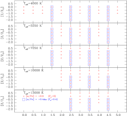
Figure 1: Typical coverage in the atmospheric parameters, and $\Gamma_{\alpha}$ of the 1-Å resolution spectra used in this study. The filled-triangles are for chemical compositions with solar abundance ratios [$\alpha$/Fe]=0 ($\Gamma_{\alpha}$=0), whereas the open-squares are $\alpha$-enhanced mixtures with [$\alpha$/Fe]=+0.4 dex ($\Gamma_{\alpha}$=0.4).

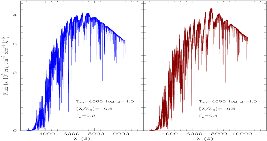
Figure 2: Two theoretical spectra of the Munari et al. (2005) library. Left-hand panel: spectral energy distribution F_λ for the star with $T_{{\rm eff}}$=4000 K, $\log g$=4.5, ${\rm[Z/Z_{\odot}]}$=–0.5, $\Gamma_{\alpha}$=0. The wavelength is in Å. F_λ is in ${\rm erg\leavevmode\nobreak\ sec^{-1}cm^{-2}\AA^{-1}}$ and the resolution is 1Å. Right-hand panel: the same but for $\Gamma_{\alpha}$=0.4.

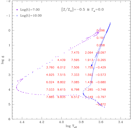
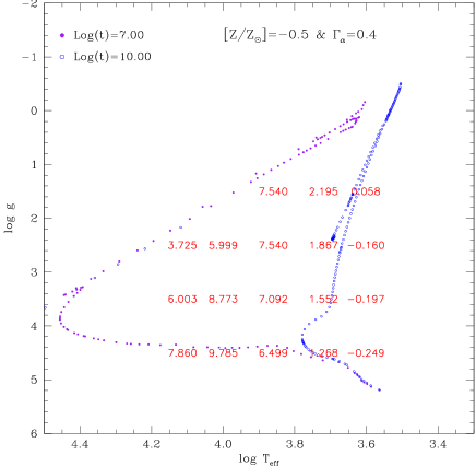
Figure 3: Left Panel Variation of ${\rm H}\beta$ from 1-Å resolution spectra across the HR-diagram in the $\log g$ versus $\log T_{{\rm eff}}$ plane. Each value of ${\rm H}\beta$ corresponds to a star (theoretical spectrum) of given $\log g$, $\log T_{{\rm eff}}$ and ${\rm[Z/Z_{\odot}]}$. The case under consideration is for ${\rm[Z/Z_{\odot}]}$=–0.5 and $\Gamma_{\alpha}$=0. In the same diagram we also plot two isochrones of the Padova Library with the same metallicity (Z=0.008) and ages of 0.01 and 10 Gyr. Right Panel: The same as in the left panel but for $\Gamma_{\alpha}$=0.4.

The temperature, gravity and metallicity coverage of the body of stellar spectra in usage here is summarized in Fig. 1 (as already mentioned in the case of the highest metallicity and $\alpha$-enhanced spectra, the temperature interval is smaller). Each panel is for a different effective temperature as indicated. The symbols show the combination of metallicity, expressed here in spectroscopic notation as ${\rm[Z/Z_{\odot}]}=log({\rm Z/Z_{\odot}})$, and gravity ($\log g$) for which a spectrum has been calculated. The triangles are for $\Gamma_{\alpha}$=0 whereas the squares are for $\Gamma_{\alpha}$=0.4. The parameters span the following ranges: two values of [$\alpha$/Fe] (or $\Gamma_{\alpha}$), i.e. [$\alpha$/Fe]=0 and +0.4 dex; six values of ${\rm[Z/Z_{\odot}]}$, i.e. –2.0, –1.5, –1.0, –0.5, 0 and 0.5 for [$\alpha$/Fe]=0, and five values (${\rm[Z/Z_{\odot}]}$=–2.0, –1.5, –1.0, –0.5 and 0) for [$\alpha$/Fe]=+0.4 dex; five values of $T_{{\rm eff}}$, i.e. 4000, 5250, 7250, 10000 and 13000 K for most of the spectra, they are reduced to three values (4000, 5250 and 7250 K) for [$\alpha$/Fe]=+0.4 dex and ${\rm[Z/Z_{\odot}]}$=0; finally eleven values of $\log g$ going from 0 to 5.0 in steps 0.5. The spectral grid is only a sub-set of the original model atmosphere grid, however fully adequate to the purposes of this study. The range of wavelength in each spectrum goes from 2500Å to 10500Å with resolution of 1Å. The flux F_λ is in ${\rm erg\leavevmode\nobreak\ sec^{-1}cm^{-2}\AA^{-1}}$. In Fig. 2 we show for the sake of illustration the spectral energy distribution for the model with $T_{{\rm eff}}$=4000 K, $\log g$=4.5, ${\rm[Z/Z_{\odot}]}$=–0.5, micro-turbulence velocity $k$=2 km/sec, and $\Gamma_{\alpha}$=0 (left panel) and 0.4 (right panel). It fairly represents the case of a cool-dwarf star.

4.2 Indices from 1-Å resolution spectra

With the aid of equations (1) and (2) and the pass-bands of Trager et al. (1998) we filter the energy distribution of each star in our grids and derive the indices. They are not strictly equivalent to the Lick system because the spectra in usage have 1-Å resolution, whereas those on the Lick system have significantly smaller resolution (approximately 8.4Å) that also depends on the wavelength interval (see Worthey & Ottaviani 1997, for all details). This case will be considered in detail in Section 4.4.

The data for the whole sets of indices are not displayed but they are partly given in and partly recovered from Tables A.1 through A.5 to be described in Appendix A. We limit ourselves to show in Figs. 3 the variation of the index ${\rm H}\beta$ across the HR-diagram for the case with ${\rm[Z/Z_{\odot}]}$=–0.5 and $\Gamma_{\alpha}$=0 and 0.4. In the same diagram we also plot two isochrones with the same metal content taken from the Padova Library (Girardi private communication): the ages are 0.01 Gyr and 10 Gyr. The grids of calibrating stars cover most of the HR-diagram in which real stars are found.

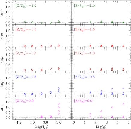
Figure 4: 1-Å resolution spectra. Variations of the index ${\rm H}\beta$ passing from solar to $\alpha$-enhanced chemical mixture. We plot the difference $\left(\delta I\right)_{\mbox{$T_{{\rm eff}}$},g,{\rm[Z/Z_{\odot}]}}$ as a function of the atmospheric parameters as indicated. Left-hand panels: for each $\log T_{{\rm eff}}$ $\delta$H$\beta$ increases with $\log g$. Right-hand panels: for each $\log g$ $\delta$H$\beta$ decreases with $\log T_{{\rm eff}}$.

4.3 Response functions for 1-Å resolution spectra

It is worth of interest here to present the analogue of the Tripicco & Bell (1995) $\mathcal{RF}$s, the only major difference is that they cannot be evaluated for separate increases in the abundance of individual species [$\alpha_{i}/{\rm Fe}$] but only for all elements enhanced with respect to the solar value lumped together. Now the dependence of the $\mathcal{RF}$s on temperature, gravity, metallicity and enhancement can be evaluated in detail. This was not the case with the Tripicco & Bell (1995) calibration which stood on three stars with solar metallicity. We start calculating the differences

$$\left(\delta I\right)_{\mbox{$T_{{\rm eff}}$},g,{\rm[Z/Z_{\odot}]}}=I_{{\rm enh}}-I_{{\rm sol}}$$ (14)

taken at fixed $\log T_{{\rm eff}}$, $\log g$ and metallicity (${\rm[Z/Z_{\odot}]}$) and varying $\Gamma_{\alpha}$ from 0 to 0.4, whose corresponding indices are indicated as $I_{{\rm sol}}$ and $I_{{\rm enh}}$, respectively. The differences for the whole sets of values are given in Tables A.1–A.5 for ${\rm[Z/Z_{\odot}]}$=–2.0, –1.5, –1.0, –0.5 and 0, respectively.

In the ten panels of Fig. 4 we show the case of ${\rm H}\beta$. Each panel displays the variation of ${\rm H}\beta$ at changing $\log T_{{\rm eff}}$ (left panels) and/or $\log g$ (right panels). We note that, for any metallicity and passing from $\Gamma_{\alpha}$=0 to 0.4: (i) at given $\log T_{{\rm eff}}$ $\delta$${\rm H}\beta$ increases at increasing $\log g$; (ii) at given $\log g$ $\delta$${\rm H}\beta$ increases at decreasing $\log T_{{\rm eff}}$. For most cases $\delta$${\rm H}\beta$ is positive, i.e. the index ${\rm H}\beta$ increases at increasing $\Gamma_{\alpha}$ or, in other words, ${\rm H}\beta$ for $\alpha$-enhanced mixtures is greater than the solar case, keeping all other parameters constant. The increase is always significant, say approximately 0.1$\div$0.2, but it can amount to nearly 1.4 for stars of low $T_{{\rm eff}}$ and high gravity, roughly in the intervals covered by cool-dwarf and old turn-off stars, which are the most interesting in view of the forthcoming applications.

Why such an increase with $\alpha$? The answer lies in relative variation of F_l and F_c. In the case of ${\rm H}\beta$ (our prototype index) we derive the variation $\left(\delta I\right)$ passing from solar to $\alpha$-enhanced mixtures. Upon differentiating the index with respect to F_l and F_c ($\frac{\partial I}{\partial{\rm F}_{l}}$=–$\frac{1}{{\rm F}_{c}}\Delta\lambda$ and $\frac{\partial I}{\partial{\rm F}_{c}}$=$\frac{{\rm F}_{l}}{{\rm F}_{c}^{2}}\Delta\lambda$) we obtain

$$\left(\delta I\right)=\Delta\lambda\left(\frac{{\rm F}_{l}}{{\rm F}_{c}}\right)_{{\rm sol}}\left[{\Delta{\rm ln\leavevmode\nobreak\ F}_{c}}-{\Delta{\rm ln\leavevmode\nobreak\ F}_{l}}\right]$$ (15)

where $\Delta{\rm ln\leavevmode\nobreak\ F}_{l}$ and $\Delta{\rm ln\leavevmode\nobreak\ F}_{c}$ are the differences in the line and continuum fluxes passing from enhanced to solar. Plugging the values of F_l and F_c as appropriate, it turns out that the index increases with $\alpha$. What happens is best illustrated in Fig. 5 which, limited to the case of a typical cool-dwarf with $T_{{\rm eff}}$=4000, $\log g$=4.5 and ${\rm[Z/Z_{\odot}]}$=–0.5 (Z=0.008), shows how the index ${\rm H}\beta$ is built up and how it varies passing from $\Gamma_{\alpha}$=0 to $\Gamma_{\alpha}$=0.4. First in the bottom panel we display the ratio F${}_{\lambda,{\rm enh}}/{\rm F}_{\lambda,\odot}$ and the pass-bands defining the index ${\rm H}\beta$. The absorption in the $\alpha$-enhanced spectrum is significantly larger than in the solar-scaled one. The effect is larger in the blue pseudo-continuum and central band than in the red pseudo-continuum. This means that $\alpha$-enhanced mixtures distort the spectrum in such a way that simple predictions cannot be made. This is due to the contribution of hundreds of molecular and atomic lines falling into the spectral regions over which the index is defined. Secondly, in the upper panel we show the spectral energy distribution of the solar-scaled (solid line) and $\alpha$-enhanced (dotted line) spectrum and once more the pass-bands for ${\rm H}\beta$. The open-circles and the big empty star show the mean fluxes in the three pass-bands and the interpolation of the pseudo-continuum to derive F_c in the case of solar-scaled spectrum. The filled-triangles and the empty pentagon are the same but for the $\alpha$-enhanced mixture. The increase of ${\rm H}\beta$ passing from solar to $\alpha$-enhanced abundance ratios is straightforward.

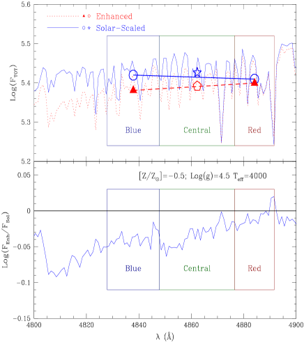
Figure 5: 1-Å resolution spectra. Building-up of the index ${\rm H}\beta$ in the cool-dwarf with $T_{{\rm eff}}$=4000, $\log g$=4.5 and ${\rm[Z/Z_{\odot}]}$=–0.5 both for the solar scaled and the total enhancement factor $\Gamma_{\alpha}$=0.4. The bottom panel shows the ratio F${}_{\lambda,{\rm enh}}/$F_λ,⊙. The absorption in the $\alpha$-enhanced spectrum is significantly larger than the solar-scaled one. The effect is larger in the blue wing of the pseudo-continuum and central band than in the red pseudo-continuum. The upper panel shows the spectral energy distribution of the solar-scaled (solid line) and $\alpha$-enhanced (dotted line) spectrum and the pass-bands defining the index ${\rm H}\beta$. The open-circles and star show the mean fluxes in the three pass-band and the interpolation of the pseudo-continuum to derive F_c in the case of solar scaled spectrum. The filled-triangles and pentagon are the same but for the $\alpha$-enhanced mixture. The increase of ${\rm H}\beta$ passing from solar to $\alpha$-enhanced abundance ratios is straightforward.

With the differences $\left(\delta I\right)$, the equivalent of the Tripicco & Bell (1995) $\mathcal{RF}$s [i.e. ${\rm R}_{0.3}(X_{i})$s] is

$${\rm R}_{0.4}(\alpha)=\frac{1}{I_{{\rm sol}}}\,\frac{I_{{\rm enh}}-I_{{\rm sol}}}{\Delta[\alpha/{\rm Fe}]}\,0.4$$ (16)

where the symbol $\alpha$ reminds the reader that only variations for the all elements enhanced at a time are available (the products in equations (12) and (13) would extend over one term only). Work is in progress to exactly repeat the analysis made by Tripicco & Bell (1995), i.e. to provide partial $\mathcal{RF}$s by separately enhancing individual elements at a time. This would improve upon the $\mathcal{RF}$s and yet maintain alive the $\mathcal{FF}$s until high-resolution spectra will become a general tool.

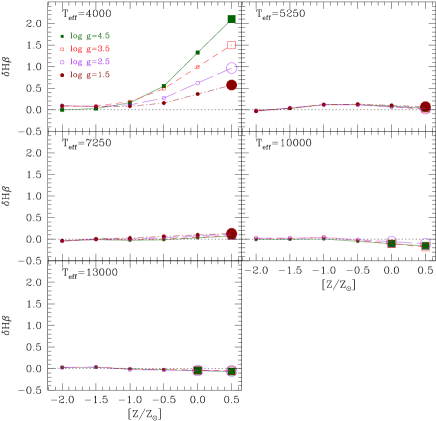
Figure 6: 1-Å resolution spectra. The variation $\delta\mbox{${\rm H}\beta$}$ as a function of the metallicity ${\rm[Z/Z_{\odot}]}$ at fixed $\log T_{{\rm eff}}$ and $\log g$ as indicated. In each panel the big symbols display the value of $\delta\mbox{${\rm H}\beta$}$ linearly extrapolated to the metallicity ${\rm[Z/Z_{\odot}]}$=0 for T$\leq$7250 K and up to 0.5 for T=1000 and 13000 K.

Having done that, for the sake of a preliminary investigation of the whole subject, we linearly extrapolate the results obtained for ${\rm[Z/Z_{\odot}]}$=–2.0, –1.5, –1.0, –0.5 and 0 to the higher value of metallicity, i.e. ${\rm[Z/Z_{\odot}]}$=0.5 for the temperatures lower than 10000 K and also to ${\rm[Z/Z_{\odot}]}$=0 and 0.5 for the temperatures of 10000 and 13000 K.

The extrapolation is safe, because $\left(\delta I\right)$=$I_{{\rm enh}}$–$I_{{\rm sol}}$ smoothly change with the metallicity at given $\log T_{{\rm eff}}$ and $\log g$. Limited to the case of ${\rm H}\beta$, this is shown in Fig. 6. The dependence is almost linear and nearly insensitive to gravity for $T_{{\rm eff}}$=5250, 7250, 10000 and 13000 K. The case of $T_{{\rm eff}}$=4000 deserves little attention, because $\delta\mbox{${\rm H}\beta$}$ tends to increase with ${\rm[Z/Z_{\odot}]}$ and gravity. Adopting the simple linear extrapolation on ${\rm[Z/Z_{\odot}]}$, we probably underestimate $\delta\mbox{${\rm H}\beta$}$ for the high metallicities.

4.4 Indices and response functions at the Lick resolution

The 1-Å resolution spectra have been degraded to the resolution of the Lick system following the procedure and the FWHM of Worthey & Ottaviani (1997). The new spectral energy distribution of each star in the calibrating grid have been filtered to derive the indices and the whole procedure described in Section 4.3 has been repeated. The data are given in Tables A.6–A.10 of Appendix A. These are the analogue of Tables A.1 through A.5. For the sake of comparison we show in Fig. 7 the differences $\left(\delta I\right)_{\mbox{$T_{{\rm eff}}$},g,{\rm[Z/Z_{\odot}]}}=I_{{\rm enh}}-I_{{\rm sol}}$. In general, the new $\left(\delta I\right)_{\mbox{$T_{{\rm eff}}$},g,{\rm[Z/Z_{\odot}]}}$ share the same trends as in the previous case, been however only slightly smaller. The most noticeable change is for ${\rm H}\beta$, whose largest $\left(\delta I\right)$ amounts to 1.1 instead of 1.4 for the case of a cool-dwarf ($T_{{\rm eff}}$=4000, $\log g$=4.5) and ${\rm[Z/Z_{\odot}]}$=0. Also in this case we linearly extrapolate the data to higher values of the metallicity for the sake of preliminary investigation. Indices and $\left(\delta I\right)$ fully consistent with the Lick system will be used in the discussion below.

Figure 7: The same as in Fig. 4 but for spectra degraded to the resolution of the Lick system. The details are given in Section 4.4. In the various panels we show the variations of the index ${\rm H}\beta$ passing from solar to $\alpha$-enhanced chemical mixture. We plot the difference $\left(\delta I\right)_{\mbox{$T_{{\rm eff}}$},g,{\rm[Z/Z_{\odot}]}}$ as a function of the atmospheric parameters as indicated. Left-hand panels: for each $T_{{\rm eff}}$ $\delta$H$\beta$ increases with $\log g$. Right-hand panels: for each $\log g$ $\delta$H$\beta$ decreases with $\log T_{{\rm eff}}$.

5 SSP indices from $\mathcal{FF}_{{\bf S}}$ and new $\mathcal{RF}_{{\bf S}}$

Owing to the large body of data and synthetic indices on the Lick system, it might be worth of interest to derive indices still based on the $\mathcal{FF}$s but in which the old $\mathcal{RF}$s are replaced by the new ones. This means that indices for solar scaled mixture are calculated as amply described in TC04, whereas those for $\Gamma_{\alpha}$$>$0 are obtained according to the following equation

$$I_{i,{\rm enh}}=I_{i,{\rm sol}}+\delta\mathcal{I}_{i}$$ (17)

where $I_{i,{\rm sol}}$ is the solar-scaled index of the generic star in the SSP and $I_{i,{\rm enh}}$ the is same but corrected for enhancement by $\delta\mathcal{I}_{i}$. This is derived by linearly interpolating both in $\log g$ and $\log T_{{\rm eff}}$ the new $\mathcal{RF}$s (listed in Tables A.6–A.10) and taking into account the enhancement-metallicity relationship discussed in Section 2.2.

5.1 Definition of SSP indices

The integrated indices of SSPs can be derived in the following way. We start from the flux in the absorption-line of the generic star of the SSP, F_l,i

$${\rm F}_{l,i} = {\rm F}_{c,i}\left(1-\frac{I_{l,i}}{\Delta\lambda}\right)\,\,\,(EW)$$ (18)

$${\rm F}_{l,i} = {\rm F}_{c,i}10^{-0.4I_{l,i}}\,\,\,(Mag)$$ (19)

where $I_{l,i}$ is the index derived from the $\mathcal{FF}$s using the $\log T_{{\rm eff}}$, $\log g$ and chemical composition of the star, and, in the case of $\alpha$-enhancement, also corrected according to equation (17). F_c,i is the pseudo-continuum flux, F_l,i is the flux in the pass-band and $\Delta\lambda$ is the same as in equation (1). The flux F_c,i is calculated by interpolating to the central wavelength of the absorption-line, the fluxes in the midpoints of the red and blue pseudo-continua bracketing the line (Worthey et al. 1994).

To calculate the flux F_c,i of a generic star one needs the theoretical spectrum of the same star. To be able to compare our results based on the new $\mathcal{RF}$s with the old ones by Trager et al. (2000b), Thomas et al. (2003a) and TC04 based on low-resolution spectra, we have to make use of stellar spectra with similar resolution. Therefore we leave aside the library of high-resolution spectra of Munari et al. (2005) and adopt the low-resolution one amalgamated by Girardi et al. (2002) and adopted by TC04. As the backbone of this library are the Kurucz ATLAS9 model atmospheres and stellar spectra, there is partial consistency between the spectra adopted to evaluate the pseudo-continuum and the 1-Å resolution spectra adopted to derive the new $\mathcal{RF}$s.

Known the fluxes F_l,i and F_c,i for a single star, we weight its contribution to the integrated value on the relative number of stars of the same type. Therefore the integrated index is given by

$$I_{l}^{{\rm SSP}} = \Delta\lambda\left(1-\frac{\sum_{i}{\rm F}_{l,i}{\rm N}_{i}}{\sum_{i}{\rm F}_{c,i}{\rm N}_{i}}\right)\,\,\,(EW)$$ (20)

$$I_{l}^{{\rm SSP}} = -2.5\log\left(\frac{\sum_{i}{\rm F}_{l,i}{\rm N}_{i}}{\sum_{i}{\rm F}_{c,i}{\rm N}_{i}}\right)\,\,\,\ (Mag)$$ (21)

where ${\rm N}_{i}$ is the number of stars in the bin.

When computing actual SSPs, single stars are identified to the isochrone elemental bins defined in such a way that all relevant quantities, i.e. luminosity, $\log T_{{\rm eff}}$, $\log g$ and mass vary by small amounts. In particular, the number of stars in an isochrone bin is given by

$${\rm N}_{i}=\int_{m_{a}}^{m_{b}}\phi(m)dm$$ (22)

where $m_{a}$ and $m_{b}$ are the minimum and maximum star mass in the bin and $\phi(m)$ is the mass function in number. These are the equations adopted to calculate the indices of SSPs.

Finally, in view of the discussion below it is worth reminding the reader the definition of two indices that are commonly used but which do not belong to the original Lick system. They are ${\rm\langle Fe\rangle}$ and ${\rm[MgFe]}$

$${\rm\langle Fe\rangle} = 0.5\times(Fe5270+Fe5335)$$

$${\rm[MgFe]} = \sqrt{\mbox{${\rm Mgb}$}\times(0.5\times Fe5270+0.5\times Fe5335)}$$

5.2 Stellar models and isochrones

For the purposes of this study, we adopt the Padova Library of stellar models and companion isochrones according to the release by Girardi et al. (2000). This set of stellar models/isochrones differs from the classical one by Bertelli et al. (1994) for the efficiency of convective overshooting and the prescription for the mass-loss rate along the asymptotic red giant branch (AGB) phase. The stellar models extend from the zero-age mean sequence (ZAMS) up to either the start of the thermally pulsing AGB phase (TP-AGB) or carbon ignition. No details on the stellar models are given here; they can be found in Girardi et al. (2000) and Girardi et al. (2002). Suffice it to mention that: (i) in low-mass stars passing from the tip of red giant branch (T-RGB) to the horizontal branch (HB) or clump, mass-loss by stellar winds is included according to the Reimers (1975) rate with $\eta$=0.45; (ii) the whole TP-AGB phase is included in the isochrones with ages older than 0.1 Gyr according to the algorithm of Girardi & Bertelli (1998) and the mass-loss rate of Vassiliadis & Wood (1993); (iii) four chemical compositions are considered as listed in Table 4.

Table 4: Chemical composition as a function of metallicity for the SSPs in use.

Z	Y	X
0.008	0.248	0.7440
0.019	0.273	0.7080
0.040	0.320	0.6400
0.070	0.338	0.5430

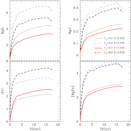
Figure 8: Indices on the Lick resolution calculated with the $\mathcal{FF}$s and the new $\mathcal{RF}$s. The panels show the temporal variation of four different indices.

Figure 9: The same as Fig. 8 but for the Balmer Lick indices.

5.3 Results for SSP indices on the Lick resolution

Going into a detailed description of the dependence of the absorption-line indices for SSPs on age, chemical composition and $\Gamma_{\alpha}$, is beyond the scope of this study. Suffice it to show in Figs. 8 and 9 the temporal evolution of nine important indices, i.e. ${\rm Mgb}$, ${\rm Mg2}$, ${\rm\langle Fe\rangle}$, ${\rm[MgFe]}$, and the Balmer Lick ${\rm H}\beta$, ${\rm H}\gamma{\rm F}$, ${\rm H}\delta{\rm F}$, ${\rm H}\gamma{\rm A}$ and ${\rm H}\delta{\rm A}$, for the following combinations of metallicity and $\Gamma_{\alpha}$, namely Z=0.008 (solid lines) and Z=0.070 (broken lines), $\Gamma_{\alpha}$=0. (heavy lines) and $\Gamma_{\alpha}$=0.4 (light lines). The age goes from 0.01 to 18 Gyr. These results are very similar albeit not identical to those found by TC04 adopting the same library of stellar spectra, the Worthey et al. (1994) $\mathcal{FF}$s, the old $\mathcal{RF}$s of Tripicco & Bell (1995) and the algorithm of Trager et al. (2000b). Finally, we note that the most controversial result in the studies by TC04 and Tantalo & Chiosi (2004b), i.e. the increase of ${\rm H}\beta$ with [$\alpha$/Fe] (and/or $\Gamma_{Z}$ and/or $\Gamma_{\alpha}$) at fixed age and metallicity, is recovered by the present analysis.

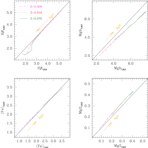
Figure 10: Indices on the Lick resolution: comparison between ${\rm H}\beta$ (top-left panel), ${\rm Mgb}$ (top-right panel), ${\rm\langle Fe\rangle}$ (bottom-left panel) and ${\rm Mg2}$ (bottom-right panel) calculated with the $\mathcal{FF}$s of Worthey et al. (1994) but different $\mathcal{RF}$s and definition of enhancement. The indices shortly indicated as $I_{{\rm O}\mathcal{RF}}$ are calculated with the first definition of enhancement ($\Gamma_{Z}$=0.25) the old $\mathcal{RF}$s by Tripicco & Bell (1995) and the algorithm of equation (12). The indices whereas $I_{{\rm N}\mathcal{RF}}$ are calculated with the second definition of enhancement ($\Gamma_{\alpha}$=0.4) the $\mathcal{RF}$s and equation (17). Both groups have the same elements enhanced by [$\alpha$/Fe]=+0.4 dex. The corresponding abundances are given in Tables 1 and 2. Finally, three different metallicities are considered as indicated.

5.4 Passing from old to new $\mathcal{RF}$s

Comparing the present results with previous ones in literature is not an easy task because the strict analogues do not exist. In brief, the models by Trager et al. (2000b, a), Maraston et al. (2003), Thomas et al. (2003a), Thomas et al. (2003b), Thomas & Maraston (2003) and TC04 are calculated with the definition of enhancement at constant Z, the classical $\mathcal{FF}$s of Worthey et al. (1994), the old $\mathcal{RF}$s of Tripicco & Bell (1995) and either equation (12) or (13) to pass from solar-scaled to $\alpha$-enhanced mixtures. The present models adopt the definition of enhancement at increasing Z, the classical $\mathcal{FF}$s of Worthey et al. (1994) the new $\mathcal{RF}$s calculated in this work and equation (17) to pass from solar-scaled to $\alpha$ enhanced indices.

In addition to this, there are differences arising from the quality of the spectra for the calibrating stars adopted by Tripicco & Bell (1995) and Munari et al. (2005). Owing to the many improvements in the physics of stellar atmospheres introduced by Munari et al. (2005) and Castelli & Kurucz (2004), the more recent compilations for the solar abundances and many other details that are shortly summarized in Section 4.1, the new $\mathcal{RF}$s likely supersede the old ones.

Despite these major drawbacks, it might be useful to compare the present models, shortly indicated as $I_{{\rm N}\mathcal{RF}}$, with those calculated with the old procedure, shortly indicated as $I_{{\rm O}\mathcal{RF}}$. These latter models have been explicitly calculated with the abundances listed in Table 1, i.e. by using the same enhancement ([$\alpha$/Fe]=+0.4 dex) but the definition at constant Z (i.e. $\Gamma$=0.25 and $\Gamma_{\alpha}$=0.4), the Tripicco & Bell (1995) $\mathcal{RF}$s and equation (12).

For the sake of brevity, we compare four indices, namely ${\rm H}\beta$, ${\rm Mgb}$, ${\rm\langle Fe\rangle}$ and ${\rm Mg2}$, for three metallicities (Z=0.008, 0.019 and 0.070) and $\Gamma_{\alpha}$ goes from 0 to 0.4 (the same values hold good for both definitions of total enhancement). This choice for the metallicity will allow us to check cases for which the $\mathcal{RF}$s have been extrapolated. Furthermore passing from the $I_{{\rm O}\mathcal{RF}}$ to the $I_{{\rm N}\mathcal{RF}}$ at given Z we have also taken into account the correlation between $\Gamma_{\alpha}$ and Z (and/or [M/H]) discussed in Section 2.2 (see Table 3). The correlations between $I_{{\rm O}\mathcal{RF}}$ and $I_{{\rm N}\mathcal{RF}}$ are shown in Fig. 10. In each panel three groups of models are displayed whose metallicity increases going from bottom-left to top-right, whereas the age increases as indicated. Along each curve the age goes from 1 to 18 Gyr as in Figs. 8 and 9.

For ${\rm\langle Fe\rangle}$ there is no significant difference between the two groups; ${\rm Mgb}$_NRF is systematically lower than ${\rm Mgb}$_ORF by 0.2Å to as much as 0.4Å at increasing age and/or metallicity; ${\rm Mg2}$_NRF tends to become larger than ${\rm Mg2}$_ORF at increasing age by as much as approximately 15 per cent. We suspect that for both indices the offset is due to differences in the stellar spectra that are difficult to pin down.

Finally, in the case of ${\rm H}\beta$ there is coincidence independently of the metallicity and definition of enhancement for ages younger than 3 Gyr, whereas for older ages ${\rm H}\beta$_ORF is larger than ${\rm H}\beta$_NRF and the difference increasing with metallicity. In the age range where the largest deviation occurs, the maximum difference amounts to approximately 30 per cent. Careful inspection of the data reveals that the difference mostly originates from correcting algorithm in usage when applied to elements for which the $\mathcal{RF}$ is strong. Recalling that the indices $I_{{\rm O}\mathcal{RF}}$ are calculated with [Ti/Fe]=0.40 (that corresponds to [Ti/H]=+0.1541), one of the elements with the strongest $\mathcal{RF}$ in Tripicco & Bell (1995) tabulation, the excess of ${\rm H}\beta$_ORF over ${\rm H}\beta$_NRF is most probably due to the correcting algorithm of equation (12) which tends to diverge whenever [$X_{i}$/Fe] or [$X_{i}/{\rm H}$]/0.3 and ${\rm R}_{0.3}(X_{i})$ are high (see equation 12). In the case of ${\rm H}\beta$_NRF the correction with respect to solar values is smaller (even though sizable) because of the linearity of the algorithm in usage. For more details on this subject the reader is referred to the discussion by TC04.

From this comparison we learn that:

(i) In general, there seems to be overall agreement between the two groups of indices despite the large difference in the definition of enhancement. As the case at increasing Z requires the re-scaling of the metallicity to lower values, the results eventually get close to those at constant Z which implies a decrease in all elements that are not enhanced (Fe, in particular).

(ii) The new $\mathcal{RF}$s take into account effects that would otherwise be missed, such as the dependence on the metallicity.

(iii) The new $\mathcal{RF}$s for some indices and some stars, e.g. ${\rm H}\beta$ for cool-dwarfs, have the opposite dependence on $\Gamma_{\alpha}$ as compared to that predicted by Tripicco & Bell (1995). The result stems from the modern physical input of the new spectra.

No better comparison can be made at the present time, because we would need stellar spectra with abundances of elemental species increased one-by-one to derive the strict analogue of the $\mathcal{RF}$s by Tripicco & Bell (1995) and spectra with enhanced composition according to the constant Z scheme. All this is still out of reach for obvious reasons.

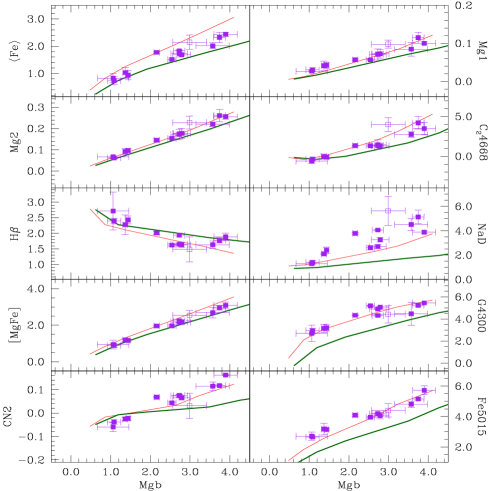
Figure 11: The ${\rm Mgb}$ index versus ten different indices on the Lick resolution calculated with metallicities typical of globular clusters. The thin-solid lines are the models with solar-scaled pattern of abundances, whereas the thick-solid are the models with $\Gamma_{\alpha}$=0.4. Along each line are shown the indices of SSPs with the same age, $\sim$12 Gyr and different metallicity from ${\rm[Z/Z_{\odot}]}$=–2 (Z$\sim$0.0001) to 0 (Z$\sim$0.019). These models are calculated with the classical $\mathcal{FF}$s and the new $\mathcal{RF}$s. The filled-squares are the globular cluster data, the open-square is the galactic bulge from Puzia et al. (2002).

6 Comparison with globular clusters

It is worth checking whether the present indices can reproduce the data for the globular clusters.

To this aim we have taken the sample of galactic globular clusters and bulge compiled by Puzia et al. (2002) for which indices on the Lick system have been measured. To analyze this sample we adopt the isochrones of the Padova Library with chemical composition typical of the galactic globular clusters (Girardi et al. 2000), and derive the indices using the classical $\mathcal{FF}$s and the new $\mathcal{RF}$s as described in Section 5. The metallicity-enhancement relation is taken into account when comparing indices for solar-scaled and $\alpha$-enhanced mixtures. The results are shown in Fig. 11 for a number of indices. Each line show the expected correlation between two indices at fixed age and varying metallicity. The age under consideration is that typical of globular clusters, i.e. 12 Gyr. The metallicity increases from ${\rm[Z/Z_{\odot}]}$=–2.0 (Z$\sim$0.0001) to ${\rm[Z/Z_{\odot}]}$=0 (Z$\sim$0.019) moving from bottom left to top right. The thin-solid lines are the models with solar-scaled pattern of abundances, whereas the thick-solid are the models with $\Gamma_{\alpha}$=0.40. Despite the fact that these indices were not particularly designed to match the globular clusters, the overall agreement is satisfactory. The new indices are of the same quality as those in TC04 and Thomas et al. (2003a). In general, the agreement is better for the solar-scaled mixture even if values of $\Gamma_{\alpha}$ in the range from 0 to 0.4 cannot be excluded. The index ${\rm NaD}$ depart from the observational value both in Thomas et al. (2003a), TC04 and here.

Table 5: Ages, metallicities and [$\alpha$/Fe] for the sample of Galactic Globular Clusters by Puzia et al. (2002). Columns (2) through (5) are estimates of the parameters based on the colour-magnitude diagrams or spectroscopic measurements; columns (6) through (8) are the results derived from the absorption line indices.

NGC	[Fe/H]CG	[$\alpha$/Fe]d	TCG	$\sigma_{T}$	[Z/H]	[$\alpha$/Fe]	Age
5927	–0.64a	—	10.0	0.7a	–0.62	0.34	12.6
6218	–1.14a	0.35	10.0	0.9a	–1.76	0.30	7.9
6284	–1.13a	—	9.5	0.4a	–1.51	0.37	8.9
6356	–0.89a	—	10.0	2.0b	–0.94	0.37	12.6
6388	–0.74a	—	10.6	2.0b	–0.91	0.06	10.0
6528	0.07b	0.11	10.0	2.0b	–0.03	0.16	12.6
6553	–0.06b	0.19	10.0	2.0b	–0.03	0.03	12.6
6624	–0.70b	—	10.6	1.4c	–0.91	0.30	12.6
6637	–0.78a	—	9.9	1.1a	–1.03	0.37	12.6
6981	–1.21a	—	8.7	0.9a	–1.74	0.34	10.0
a De Angeli et al. (2005)
b Santos & Piatti (2004)
c Salaris & Weiss (2002)
d Pritzl et al. (2005)

To further confirm the quality of the theoretical indices we derive the ages, metallicities and enhancement degree from the indices for the sub-set of this sample of globular cluster for which the same parameters are known from the colour-magnitude diagrams.

To this aim, first we select the globular clusters for which estimate of ages and metallicities (i.e. [Fe/H]) have been derived from the colour-magnitude diagrams (see De Angeli et al. 2005; Santos & Piatti 2004; Salaris & Weiss 2002; Schiavon et al. 2005). Then we consider the current estimates of enhancement (i.e. [$\alpha$/Fe]) obtained directly from stars and take these as indicators of the total degree of enhancement in each cluster (Pritzl et al. 2005, see). Table 5 lists the metal content, degree of enhancement and age together with its uncertainty we have been able to collect from literature (the sources of data are indicated). These are the values we would like to recover from the indices.

To derive metallicities, degree of enhancement and age from indices we adopt the Minimum-Distance Method originally proposed by Trager et al. (2000b) and amply described in TC04. Due to the different sensitivity of the adopted indices to each parameter we prefer to use the so-called Recursive Minimum-Distance Method .

Taking advantage of the high sensitivity of ${\rm\langle Fe\rangle}$ and ${\rm Mg2}$ to [$\alpha$/Fe] and their lower sensitivity to age and metallicity, we have apply the minimum-distance method to derive [$\alpha$/Fe] form the plane ${\rm\langle Fe\rangle}$-${\rm Mg2}$ assuming the provisional age T$\sim$13. This value, shortly indicated as $\Gamma^{0}_{\alpha}$, is used to construct the functions ${\rm H}\beta$(T,Z,$\Gamma^{0}_{\alpha}$), ${\rm\langle Fe\rangle}$(T,Z,$\Gamma^{0}_{\alpha}$) and ${\rm Mgb}$(T,Z,$\Gamma^{0}_{\alpha}$) and to solve the equations:

$$\mbox{${\rm H}\beta$}_{obs}=\mbox{${\rm H}\beta$}(T,Z,\Gamma^{0}_{\alpha})$$

$$\mbox{${\rm\langle Fe\rangle}$}_{obs}=\mbox{${\rm\langle Fe\rangle}$}(T,Z,\Gamma^{0}_{\alpha})$$

$$\mbox{${\rm Mgb}$}_{obs}=\mbox{${\rm Mgb}$}(T,Z,\Gamma^{0}_{\alpha})$$

for the age and metallicity (T and Z). The procedure is iterated till full consistency is achieved.

The results of this analysis are shown in Table 5 (columns (6) through (8) for the metallicity, [$\alpha$/Fe] and age, respectively). Metallicities, degree of enhancement and ages derived from indices fully agree with those obtained from the colour-magnitude diagrams. This holds good both for individual clusters and the mean values for the whole sample: $\langle$Age$\rangle$=11.2$\pm$1.8, $\langle$[Z/H]$\rangle$=–0.95$\pm$0.62 and $\langle$[$\alpha$/Fe]$\rangle$=0.26$\pm$0.13 .

7 Discussion and conclusions

We have generated synthetic absorption-line indices on the Lick system based on the recent library of 1-Å resolution spectra calculated by Munari et al. (2005) over a large range of atmospheric parameters ($\log T_{{\rm eff}}$, $\log g$ and [Fe/H]) and both for solar and $\alpha$-enhanced abundance ratios in the chemical composition. The main results of this study are:

(i) First we derive a modern version of the so-called $\mathcal{RF}$s of Tripicco & Bell (1995). Contrary to the previous situation in which the $\mathcal{RF}$s were known only for three stars of given $\log T_{{\rm eff}}$ and $\log g$, now the $\mathcal{RF}$s are given for large range ranges of $\log T_{{\rm eff}}$, $\log g$ and [Fe/H] (or ${\rm[Z/Z_{\odot}]}$). Not only the $\mathcal{RF}$s vary with the type of star but also with the metallicity. The effect of metallicity is important and cannot be neglected. While completing this study, similar analysis has been published by Korn et al. (2005) who strictly following the Tripicco & Bell (1995) approach, presented the $\mathcal{RF}$s for three stars (a dwarf, a turn-off and a red giant for six chemical composition). Their results are similar to ours even if the coverage of the effective temperature-gravity intervals for the reference stars is much narrower.

(ii) With the aid of the new $\mathcal{RF}$s and the $\mathcal{FF}$s of Worthey et al. (1994) indices for SSPs are calculated and compared with the old ones by TC04. But for the differences caused by the new $\mathcal{RF}$s and the kind of enhancement adopted by TC04 and here, the agreement is good thus confirming that the method adopted by TC04 to account for the effect of $\alpha$-enhancement albeit hampered by the coarse grid of calibrating stars in Tripicco & Bell (1995) was correct. The present results clearly demonstrate that not only all indices depend on the enhancement but also that ${\rm H}\beta$ increases with it as already anticipated by TC04 and contrary to what claimed by Thomas et al. (2003a, b) and only marginally admitted by Korn et al. (2005) in their recent study.

(iii) The new indices have been compared to those of galactic globular clusters for which there are independent estimates of age, metallicity and degree of enhancement and used to re-derive these basic parameters by means of the recursive minimum distance method customarily applied to galaxies. The estimates of the three key parameters from the two methods agree each other thus suggesting that the indices for SSPs we have calculated are correct.

Appendix A

Tables A.1–A.5 list the new $\mathcal{RF}$s calculated with the 1-Å resolution spectra from Munari et al. (2005) as function of $T_{{\rm eff}}$ and $\log g$ and for four different metallicities: ${\rm[Z/Z_{\odot}]}$=–2.0, –1.5, –1.0, –0.5. For each index we give the value $I_{{\rm sol}}$ for the solar abundance ratios and the difference $\left(\delta I\right)$=$I_{{\rm enh}}-I_{{\rm sol}}$ between the $\alpha$-enhanced and the solar case. The corresponding $\mathcal{RF}$s can immediately be derived from relation (16). Tables A.6–A.10 are the same but for the high-resolution spectra degraded to the Lick resolution.