VLT FORS-1 observations of NGC 6397: Evidence for mass segregation

We present (V,V-I) VLT-FORS1 observations of the Galactic Globular Cluster NGC 6397. We derive accurate color–magnitude diagrams and luminosity functions (LFs) of the cluster Main Sequence (MS) for two fields extending from a region near the centre of the cluster out to $\simeq$ 10$\arcmin$. The photometry of these fields produces a narrow MS extending down to V $\simeq$ 27, much deeper than any previous ground based study on this system and comparable to previous HST photometry. The V, V-I CMD also shows a deep white dwarf cooling sequence locus, contaminated by many field stars and spurious objects. We concentrate the present work on the analysis of the MSLFs derived for two annuli at different radial distance from the center of the cluster. Evidence of a clear-cut correlation between the slope of the observed LFs before reaching the turn-over, and the radial position of the observed fields inside the cluster area is found. We find that the LFs become flatter with decreasing radius (x $\simeq$ 0.15 for $1\arcmin<R_{1}<5.5\arcmin$; x$\simeq$ 0.24 for $5.5\arcmin<R_{2}<9.8\arcmin$ ; core radius, r_c= 0.05$\arcmin$), a trend that is consistent with the interpretation of NGC 6397 as a dynamically relaxed system. This trend is also evident in the mass function.

1 Introduction

Globular cluster stars fainter than the Main Sequence Turn-Off (MSTO) are substantially unevolved and are located along the MS according to their initial mass. Their luminosity distribution is usually described by the Initial Mass Function as modified by subsequent dynamical evolution to become the so-called Present Day Mass Function (PDMF). The precise knowledge of the Initial Mass Function is a cornestone in a variety of astrophysical problems, ranging from the physics of stars formation to the dynamical and chemical modeling of Galactic evolution. In this respect, GGCs are perhaps the best suited halo structures to investigate the faint PDMF and Initial Mass Function (IMF), and to verify the existence and size of a population of very low mass stars, possible major contributors to the dark halos in galaxies. The mass segregation then should be seen as a radial dependence of the LFs, but to verify these theoretical predictions we need to obtain a statistically significative sample of data starting from the central regions of the cluster. Until now the only instrument available to obtain a precise luminosity function of the main sequence below the turn-off at various distances from the centre of a cluster was the HST. Nowadays, this is also possible with ground based observations thanks to the large collecting area and huge resolving power of the VLT. In this work we concentrate on NGC 6397. There are several reasons for this choice: i) it is the closest cluster, hence it is possible to reach the faintest part of the MS; ii) it is a classical, old, metal-poor halo cluster, and its age constitutes a lower limit to the age of the Galaxy and, therefore, to the Universe as a whole; iii) an extended study carried out with HST on a central area over several years (see Cool et al., 1996; King et al., 1998) allowed us to separate through proper motions the cluster from the background/foreground field, and is a valuable comparison source with our data; iv) a fairly well defined white dwarf (WD) sequence is visible.
NGC 6397 is located at $\alpha=17^{h}41^{m}53^{s}$, $\delta=-53^{\circ}44^{\prime}30^{\prime\prime}$ and has a metallicity [Fe/H] = -1.82 (Carretta & Gratton, 1997), slightly higher than the fiducial most metal-poor cluster M 92 ([Fe/H] = -2.15 (Gratton et al., 1997). High-quality populated color–magnitude diagrams (CMD) have been produced in the past either from the ground (see, e.g., Alcaino et al., 1987, 1997) and from the space (Cool et al., 1996; De Marchi et al., 1995a). The distance has been recently re-determined by Reid & Gizis (1998) with a set of extreme subdwarfs from the catalogue of HIPPARCOS, obtaining $(m-M)_{0}=12.13\pm 0.15$. The reddening adopted by the authors, which is a weighted mean of the available estimates is $E(B-V)=0.18$. We will adopt these values in the following. The field of view covered by our data ranges over a 8.8^′ radius, starting at about 1^′ from the cluster center. This displacement allowed us to study the presence of mass segregation in the luminosity function on NGC  6397. The structure of the paper is as follows: Sects. 2 and 3 present the data, the reduction procedures and the V, V-I CMD. The resulting LF and MF are presented and discussed in Sects. 4 and 5. Sect. 6 summarizes the results.

2 Observations and data reduction

The observations consist of two fields (f1 and f2 in the text), including several 600 s exposures in each of the two V and I Bessel filters, taken with the standard resolution of the VLT + FORS1 (0.2 $\arcsec$/pixel) corresponding to a field of view of 6.8$\arcmin$ $\times$ 6.8 $\arcmin$ (see Table 1). The data taken in service mode in 1999 (f2) and in 2000 (f1) were retrieved electronically from the ESO-STECF archive (proposals: 63.H-0721(A) and 65.H-0531(B)).

Table 1: Journal of observations for the fields f1 and f2. N_I and N_V are the number of exposures respectively for the filter I and V; t is the exposure time in seconds.

$$\begin{array}[]{c|cc|cc}\mathrm{field}&\alpha&\delta&\mathrm{N_{I}\times\mathrm{t}}&\mathrm{N_{V}}\times t\\ \hline\cr f1&17^{h}41^{m}14.3^{s}&-53^{0}44^{\prime}27.6^{\prime\prime}&59\times 600&42\times 600\\ f2&17^{h}41^{m}03.5^{s}&-53^{0}45^{\prime}36^{\prime\prime}&11\times 600&13\times 600\end{array}$$

The two partially overlapped fields are located at $\simeq$ 5$\arcmin$ SE from the cluster center and cover a region of the cluster already observed with the HST-WFPC2 by Cool et al. (1996) (see Fig. 1). The presence of a region in common between the two ground fields and the HST fields allowed us to obtain a homogeneous calibration for the whole ground-sample.

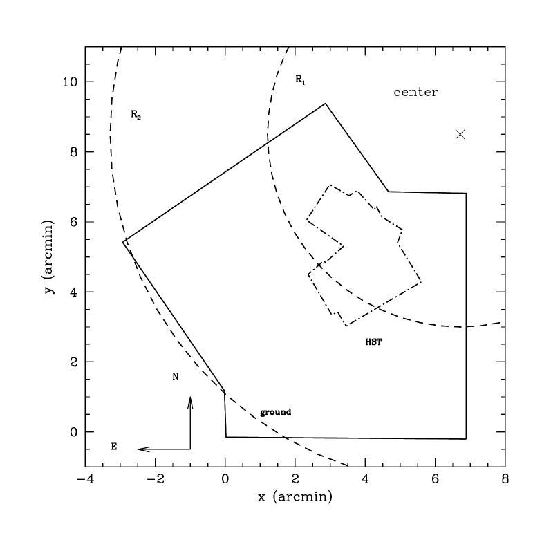
Figure 1: The location of the HST-fields (Cool et al., 1996) inside the ground-fields. The position of the center of the cluster is (6.71 $\arcmin$, 8.5 $\arcmin$). Dashed circles represent the annuli in which we divided our sample to perform data analysis (see text for further details)

Corrections to the raw data for bias, dark and flat-fielding were performed using the standard IRAF routines following the same recipe employed in the ESO-VLT pipeline. Subsequent data reduction and analysis was done by following the same procedure for both the data-sets, and using the DAOPHOT-ALLFRAME package (Stetson, 1987, Version3) with a quadratically varying point spread function (PSF).

Since our goal was to reliably detect the faintest objects in both fields, first we created two median images using all available frames in each filter of a given field, then we added these median images together to obtain the final images on which to search for objects by running the standard DAOPHOT routines. The candidates were then measured on each of the individual V and I frames and an average instrumental magnitude was derived for those recovered in at least three frames.

As our fields were affected by a large number of saturated stars and, as the photometric procedures can include those peaks in the final photometric catalogue, we decided to eliminate from the catalogue the spurious identifications before performing the data analysis. In this way, a total of 15081 and 11161 objects were detected, respectively, in the fields f1 and f2.

We used the 7059 objects in common between these two fields to optimize our photometry by computing a weighted average between the values of the magnitudes of a given star in each catalogue and to transform the frame coordinates to a common coordinate system referred to the field f2. At the end of this procedure an homogeneous set of instrumental magnitudes, color and position were obtained for a total of 19228 objects.

Conversion from instrumental magnitudes to the HST VEGAMAG standard system, which is similar to the Johnson system (Holtzman et al., 1995) was performed by using the 3559 objects in common between the two ground data sets and the catalogue from HST observations (Cool et al., 1996).

3 The Color Magnitude Diagram and the Luminosity Function

Figure 2 shows the V, V-I CMD for 16105 objects of the original catalogue for which photometric errors are: $\sigma_{I},\sigma_{V}\leq 0.15$.

Figure 2: V, V-I color-magnitude diagram for 16105 objects selected from the original catalogue ($\sigma_{I}$, $\sigma_{V}\leq 0.15$). The mean errors per interval of magnitude V are also plotted.

This figure shows the high quality of our photometric data. A very narrow MS (0.028 $\leq\sigma(V-I)\leq$ 0.15 for 19 $\leq$ V $\leq$ 25), extending down to V $\sim$ 27 is visible, much deeper than any previous ground based study (Alcaino et al., 1987, 1997) and comparable only with the most recent HST photometry (Cool et al., 1996). From the figure a deep white dwarfs cooling sequence locus is also clear, although contaminated at the faintest magnitudes by many field stars and possibly spurious objects.

3.1 The white dwarf cooling sequence

In Fig. 3 we overplot theoretical cooling sequences for 0.5, 0.7 and 0.9 M_⊙ hydrogen-rich WDs on the CMD. Theoretical cooling sequences have been obtained using the WD cooling models of Hansen et al. (1998, 1999) as described in Richer et al. (2000) and have been trasformed to apparent magnitudes and colors appropriate for NGC 6397 adopting $\mathrm{(m-M)_{0}}=12.13$ and $\mathrm{E(B-V)}=0.18$.

Since the population of WDs accumulates at lower luminosities as the age of the cluster increases, we could fix a limit to this age by looking at the location of the faintest WDs in the cooling sequence. However the high contamination by field stars in this region of the CMD does not allows us to extract precise information. By looking at the faint end of the cooling sequence (V $\simeq$ 27), the age of the oldest WDs in the cluster ranges from $\simeq$ 2 Gyr to $\simeq$ 3.8 Gyr, for WDs with mass ranging from 0.5 M_⊙ to 0.9 M_⊙ respectively.

Figure 3: Comparison of NGC 6397 cooling sequence with hydrogen-rich WD cooling sequences (solid lines) of 0.5, 0.7 and 0.9 M_⊙, obtained by using models from Hansen (1998, 1999).

3.2 The Luminosity Function

Before using the CMD to build the MSLF, we carefully selected the sample in order to keep only the bona fide real objects. In particular we found that they appear in at least 80 $\%$ of the original frames. We adopted the following selection procedure: for each field, we first built two maps (the ’weight-maps’) with the same dimension of the median images I and V used for candidate searching (see sect. 2 for details). These maps are such that the value of each pixel is the number of times the pixel appears on the stack, i.e. how many frames are stacked onto each other on that pixel, and ranges from [1 - N_max], where N_max is the total number of frames overlapped in the original median image. With this information we found, for each object, the number of frames in which it has been recovered with respect to the number of frames in which it is expected to be detected.

Figure 4 and 5 show the variation of the CMD, and the correspondent LF, with the parameters $r_{I}$ and $r_{V}$ defined, respectively, as the ratio between the number of frames in which a star has been recovered ($n_{I,V}(rec)$) and the number of the original frames available for that pixel ($n_{I,V}(frame)$):

$$r_{I,V}=\frac{{\displaystyle n_{I,V}(rec)}}{{\displaystyle n_{I,V}(frame)}}$$ (1)

In particular, for the two cases: $r_{I,V}>$ 0, and $r_{I,V}$ = 1, we are looking at: i) all the objects of the original catalogue (without any selection); ii) only the objects recovered simultaneously in all the original frames.

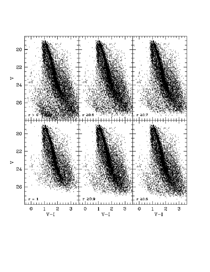
Figure 4: V, V-I color-magnitudes diagram obtained selecting the original catalogue for different values of the ratio $r=r_{I}=r_{V}$.

Figure 5: LFs obtained selecting the original photometric catalogue for different values of the ratio $r=r_{I}=r_{V}$.

An analysis of these figure shows that, by increasing the value of the parameter r, and thus decreasing the number of the selected objects in the catalogue: i) the distribution of the objects located in the region of the CMD we are interested, i.e. the MS stars with a magnitude brighter than V = 22, (the peak of the LF), does not change; ii) we mainly lose information about the faint region of the CMD and in particular for the objects located at the faint end of the cooling sequence (see the case r $>$ 0), where the photometric errors are very large ($\sigma_{I},\sigma_{V}\geq 0.3$) ; iii) for a choice of the parameter r $\geq$ 0.8 (objects of the original catalogue recovered in at least 80 $\%$ of the original frames), the CMD is very similar to that shown in Fig. 4. This last suggestion may be confirmed by the comparison between the LFs associated with the CMDs reported in Fig. 6, where open triangles represent the LF obtained from a catalogue selected for $\sigma_{I},\sigma_{V}\leq$ 0.15 and dashed line is the LF from a catalogue selected for $r\geq 0.8$.

Figure 6: Comparison between the LFs obtained from a catalogue in which the objects are selected by following two different criteria: photometric errors $\leq$ 0.15 (open triangles); number of frames in which a star has been recovered (larger than 80 $\%$) (dashed line).

4 The Main Sequence Luminosity Function

4.1 Sample selection and completeness

Since our goal in this work is to study the MSLF, in the following we will concentrate our analysis only on the region of the CMD including the MS stars. In order to select the objects located on the MS locus, we built a fiducial line assuming a Gaussian color distribution, then we determined the mean color and dispersion $\sigma$, in each magnitude interval. We accepted as MS stars only the objects for which the distance from the ridge line is $\leq$ 3 $\sigma$. Figure 7 shows the MS locus selected with this procedure. The procedure is very robust where the number of MS stars is large, while it is more uncertain below V$\sim$24 where the MS is less populated and comparable to the field contribution. However, our analysis stops at brighter magnitudes (see below) and hence the uncertainty at the faintest magnitude bins has not been taken into account. The 3-$\sigma$ selection around the MS locus ensures that almost all the MS contribution is considered while minimizing the contamination from the field. This would not affect significantly the slope of the LF but would provoke an increase in the errors. Several tests have been done with different values of sigma clipping around the MS locus, and the final 3-$\sigma$ is the optimal choice.

Figure 7: V, V-I color-magnitude diagram for our data-sample. Solid line on the MS represents the ridge line; solid lines outside the MS delimit the region of the CMD that we will use to build the MSLF.

Observed MSLFs have been created by dividing the MS in bins 0.5 mag–wide, and counting the stars in each bin, correcting for incompleteness.

The incompleteness depends on the level of crowding in the observed fields and, therefore, on their location with respect to the cluster centre. In particular, an insufficient or inappropriate correction for crowding would result in the distortion of the stellar LF for the loss or overcorrection of faint star counts. In our case, crowding is not the only source of incompleteness: the distribution in luminosity of the stars is also modified by the large number of hot pixels and bad columns affecting the original images.

The fraction of objects lost in each magnitude bin as a function of the distance from the center of the cluster has been quantitatively estimated by using the widely tested artifical star method. It consists of adding a number of artificial stars to the original frames and reducing once again the ‘artificial frames’ by adopting the same technique already adopted for the original ones.

As we were interested in verifying the photometric completeness of MS stars, we simulated artificial objects with magnitude and color appropriate for the MS. In doing this, the CMD has been divided in 0.5 V-mag bins, and for each bin the mean V and I magnitudes (derived from the MS ridge line) have been computed. Then a set of artificial stars have been simulated having the selected magnitude values.

Artificial stars were first added randomly to the reference I frame, paying attention to add only a few percent ($\leq$ 10 $\%$) of the total number of stars actually present in the frames in the magnitude bin, in order to avoid a significant enhancement of the image crowding. The same stars have then been added to the other I and V frames in the same position with the respect to the reference frame.

All pairs of V and I ‘artificial’ frames ($\simeq$ 4000 images for $\simeq$ 428543 artificial stars) were then analyzed in the same way as the original ones and a final catalogue of artificial stars has been created for each bin and compared with the catalogue of the input artificial stars.

An artificial star was considered recovered if the output magnitudes fell in the original bin and $\delta{\textrm{y}}$ $\leq$ 1.5 pixel and $\delta{\textrm{mag}}$ $\leq$ 0.25 mag. If $N_{\textrm{rec}}$ is the number of the recovered stars and $N_{\textrm{sim}}$ is the number of simulated stars, the ratio $N_{\textrm{rec}}/N_{\textrm{sim}}=\Phi$, gives the completeness in that bin for the location considered. With this approach we have built a map showing how photometric completeness varies with position in the frames.

In addition to correcting for photometric incompleteness, a reliable determination of the cluster LF requires a correction for the contamination caused by field stars. In our case, we are interested only in the change of the slope of the cluster LF with the distance from the center of the cluster. Since the field star contribution is not dependent on this distance, and appears quite homogeneous over the CMD locus considered (see Cool et al., 1996), we decided not to correct for this effect, that, however, would increase the global error on the LF.

4.2 The Luminosity Function

Figure 8 shows the V, V-I CMDs obtained for stars belonging to the two annular rings S1 and S2 located respectively at 1 $\arcmin\leq R_{1}\leq 5.5\arcmin$ and 5.5$\arcmin\leq R_{2}\leq 9.8\arcmin$ from the center of the cluster (see figure 1 for details). These two regions have been selected in order to divide the sample roughly in half and to keep most of the HST sample in the inner region. Only a small fraction of the area covered by Cool et al. (1996) has been left in the outer annulus for calibration purposes. The S1/S2 radius is also roughly equivalent to $2\times r_{h}$. In this way we are quite confident that the population in S1 is representative of the half-mass radius population.

Figure 8: Left: V, V-I color-magnitude diagram for stars in the annular rings S1 (left panel) and S2 (right panel).

Figure 9 shows the corresponding LFs before (dashed line) and after (solid line) corrections for incompleteness have been applied. In the figure error bars reflect the total error associated with each bin and include both the error on the counts and the uncertainty due to the correction for incompleteness, which is the main contributor to the global error figure:

$$\sigma^{2}\approx\frac{{\displaystyle N}}{{\displaystyle\Phi^{2}}}+\frac{{\displaystyle(1-\Phi)N^{2}}}{{\displaystyle N_{sim}\Phi^{3}}}$$ (2)

where N is the number of observed stars in each bin; $\Phi$ is the incompleteness factor and N${}_{\textrm{sim}}$ is the number of simulated stars in the bin.

This uncertainty has been estimated by assuming that the number counts follow a Poisson distribution, and the uncertainty in determining $\Phi$ is derived from a binomial distribution as shown in Bolte (1989):

$$\sigma_{N}^{2}=N$$ (3)

$$\sigma_{\Phi}^{2}\approx\frac{{\displaystyle\Phi(1-\Phi)}}{{\displaystyle N_{sim}}}$$ (4)

Figure 9: Observed luminosity functions for the two fields S1 (bottom panel) and S2 (top panel) in bins of 0.5 mag before (dashed line) and after (solid line) incompleteness corrections; error bars include both Poisson error and the uncertainty due to the correction for the incompleteness. The limit of the completeness at the magnitude I = 22.5 is also indicated for both the fields.

The actual counts, the completeness factor and the counts corrected for this factor for both the fields S1 and S2 are listed in Table 2.

Table 2: Luminosity functions for the fields S1 and S2 in the V band in 0.5 mag bins. N is the actual number of stars; $\Phi$ is the completeness factor.

$$\begin{array}[]{c|rr|rr}\lx@intercol\hfil\hfil\lx@intercol\vrule\lx@intercol&\vrule\lx@intercol\hfil\textrm{S1}\hfil\lx@intercol\vrule\lx@intercol&\vrule\lx@intercol\hfil\textrm{S2}\hfil\lx@intercol\\ \cline{1-5}\cr{\textrm{V}}&{\textrm{N}}&{\textrm{$\Phi$}}&{\textrm{N}}&{\textrm{$\Phi$}}\\ \cline{1-5}\cr 19&129&0.81&90&0.87\\ 19.5&338&0.79&279&0.87\\ 20&334&0.77&239&0.87\\ 20.5&351&0.72&334&0.86\\ 21&387&0.66&403&0.84\\ 21.5&419&0.61&468&0.81\\ 22&465&0.54&694&0.77\\ 22.5&419&0.49&673&0.75\\ 23&356&0.42&560&0.70\\ 23.5&256&0.33&499&0.65\\ 24&208&0.22&486&0.59\\ 24.5&153&0&466&0.51\\ 25&39&0&179&0.43\\ \end{array}$$

By looking at the table we can see that: a) the completeness factor depends on the distance from the center of the cluster as we expect when the crowding contribution in a field is important; b) the completeness degree never exceeds 87$\%$, also at the brightest magnitudes of the more external field, S2. This last result is a consequence of the area lost by saturated pixels. This hypothesis is confirmed from the values found for area lost in the regions S1 (saturated area $\sim$ 22 $\%$) and S2 (saturated area $\sim$ 9$\%$).

The analysis of the LFs shows that they present the same characteristics already found in other galactic globular clusters with a maximum at V $\simeq$ 22 and a slow decrease to fainter luminosities (De Marchi et al., 1995a, b; Piotto et al., 1997; Marconi et al., 1998; Andreuzzi et al., 2000, and refs. therein). It is, therefore, natural to investigate whether the effect of a radial dependence of the LF, already observed in several globular clusters (see, for instance Andreuzzi et al., 2000), is found in the present set of data, that covers a significant interval of radial distances.

The LFs for S1 and S2, after applying corrections for incompleteness and normalized to the number of stars in the peak (V = 22), are shown in Fig. 10.

Figure 10: Observed luminosity functions for the two fields S1 (solid line) and S2 (dashed line) in bins of 0.5 mag, normalized to the peak (V = 22). Error bars include both Poisson error and the uncertainty due to the correction for the incompleteness.

Inspection of this figure reveals that the two LFs have similar shapes, but different slopes, in the sense that the ratio between the bright and the faint stars is larger in S1 than in S2, in qualitative agreement with the dynamical modifications that stars in globular clusters experience, as a consequence of the energy equipartition due to two-body relaxation (Spitzer, 1987).

To confirm this suggestion we applied a linear fit to the data and found that in the range in magnitude 20 $\leq$ V $\leq$ 22, the LF for stars in S2 is steeper (x = 0.24 $\pm$ 0.02) than that for stars in S1 (x = 0.15 $\pm$ 0.07). By taking the slopes with their formal error, this difference is marginally significant. A K-S test made on the two distributions gives a probability of the two distributions to be different of 95%, i.e. a two-sigma level. However, we compared our S1 LF after correction for incompleteness with LF obtained with HST, that is much less affected by incompleteness, and found a good agreement in the slope. The LF of S1 and HST are reported in Fig. 11 where the LF of S1 is shown with a continuous line and HST with a dotted line. As will be shown below, the MF slopes derived with HST data and with S1 LF, by using the same set of models, also are in excellent agreement. These two considerations lead us to conclude that the difference in the slopes of the LF of S1 and S2 are actually significant beyond the real meaning of the formal errors.

Figure 11: Comparison between the LF of S1 (continuous line), corrected for incompleteness, and the LF of HST (dotted line). The two LFs are normalized to their respective areas.

5 The Mass Function

In order to translate the luminosities into masses and estimate the PDMF in the two annuli, we used the M/L relations of Montalban et al. (2000) and Baraffe et al. (1997). The two relations are known to be similar for our mass range ($M<0.6M_{\odot}$), as pointed out by Montalban et al. (2000) in their work (see their Fig. 20). Small differences are found in the range corresponding to the magnitude range in which our LF is drawn ($19<V<23$). Figure 12 shows the two theoretical relations in the plane (Mass-V), where V is the absolute V magnitude.

We transformed our luminosities into masses for the two annuli, both models and two metallicites: ${\textrm{[Fe/H]}}=-1.5$ and ${\textrm{[Fe/H]}}=-2.0$, since the metallicity of NGC 6397 is estimated between these two values. Then, we fit a mass function of the form $dN/dM\propto M^{-\alpha}$. A recent discussion on the form of the mass function can be found in De Marchi et al. (2000).

Figure 12: The two theoretical relations used to convert luminosities into masses. Short dashed line is for Montalban et al. (2000), while long dashed line is for Baraffe et al. (1997).

Figures 13 and 14 show the PDMF for the two annuli and the fitting relation, for the two cited metallicities. The main result is that, also for the masses, the slopes differ in the two annuli S1 and S2, for both model sets. The formal uncertainties seems to indicate that the significance of this difference is high. A difference in the slope between Montalban et al. (2000) and Baraffe et al. (1997) is also found for both metallicites, Baraffe et al. (1997) being flatter. However, this difference, given the uncertainties on the fitted slopes, is only marginally significant.

We compared our slope with the one obtained by Montalban et al. (2000) in their work using the LF from King et al. (1998) for the case ${\textrm{[Fe/H]}}=-1.5$. Our derived slope for the annulus S1, that overlaps the area covered by King et al. (1998) (see Sect. 2), is in very good agreement with the estimate of Montalban et al. (2000) ($\alpha=x+1=-1.5$ versus $\alpha=-1.51$). This is a further confirmation that the completeness correction to the LF of annulus S1, that is more uncertain, has been correctly estimated.

De Marchi et al. (2000) studied the properties of the PDMF of NGC 6397 by using a data-set obtained with HST-NICMOS and archival existing WFPC2 (V, I) data and analyzed the radial behavior of the mass function in the near-IR at two different radii, namely 3.2^′ and 4.5^′ from the cluster center, and in the optical bands out to 10^′. HST data go considerably deeper in magnitude while keeping a high sample completeness. De Marchi et al. (2000) are able to determine the MF slope down to mass values of 0.09 $\mathrm{M}_{\odot}$, finding a change in the slope at 0.3 $\mathrm{M}_{\odot}$, that becomes 0.2 $\pm$ 0.1. The VLT data-set, especially in the annulus S1, can only describe the MF down to $V=22.5$ corresponding to $M\sim 0.32M_{\odot}$. However, The MF of annulus S2 has a high degree of completeness down to $V\sim 23.5$ which corresponds to $M\sim 0.2M_{\odot}$. For this subsample, it is possible to detect the change in slope found by De Marchi et al. (2000). The slope after the change is $\alpha\sim 0.27$, with the models of Montalban et al. (2000) and $\alpha\sim 0.30$ with the models of Baraffe et al. (1997). Since our completeness correction is larger than the HST sample, and thus the slope more uncertain, we can regard the agreement as good.

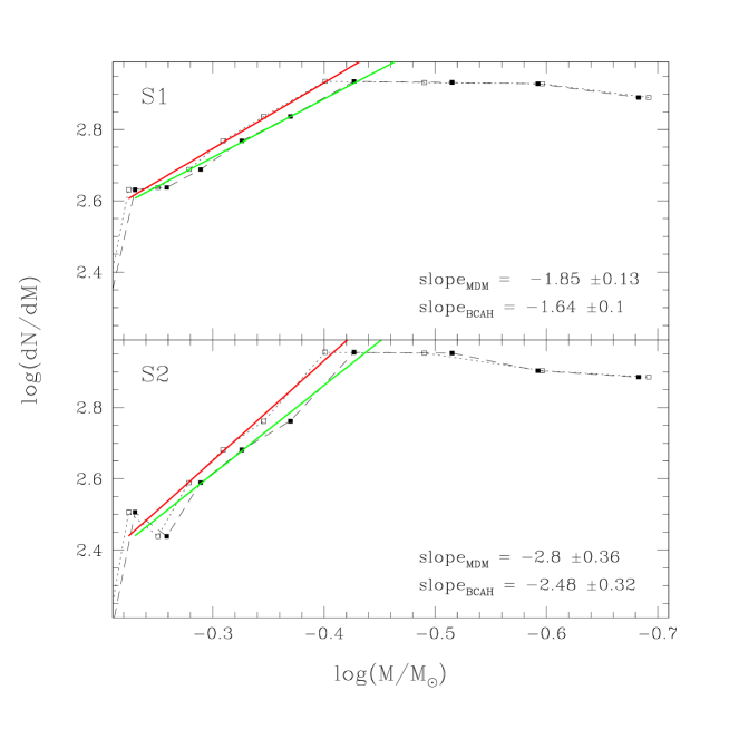
Figure 13: The MF of S1 and S2 for [Fe/H] = -1.5. The dotted line with open squares refers to Montalban et al. (2000), the dashed with block squares to Baraffe et al. (1997). The thicker continuous lines are the fitted relations.

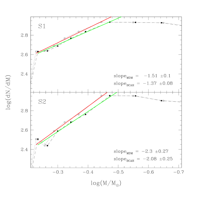
Figure 14: The MF of S1 and S2 for [Fe/H] = -2.0. Symbols are as in figure 13.

A further comparison can be made with M 92 (Andreuzzi et al., 2000), for which a similar analysis has been performed. In units of $r_{\textrm{h}}$, the authors cover a similar interval of radial distance and found a steepening of the MF before the peak, with values comparable to the ones found for NGC 6397, if homogeneous models (Baraffe et al., 1997) are used. Perhaps a trend in the sense that M 92 has a shallower overall LF can be seen and attributed to the difference in metallicity, but recent results of Pulone et al. (2003) discuss the possibility that the number of primordial binaries could play a rôle in shaping the MF, thus making the picture more complicated.

5.1 The impact of binaries on the LF of NGC 6397

In order to check the possible impact of binaries on the LF of NGC 6397, we performed the following test: first, we simulated a percentage of binary stars in each bin in mass of the MF of the annulus S2, under the simplified assumptions that the annulus S2 is made of single stars and that binaries are made of two equal mass stars. This is likely an overestimate of the effect, but the hypothesis we want to test is that, even with the maximum possible effect, binaries alone cannot explain the difference in the slopes. Then, by using backward the mass-luminosity relation of Montalban et al. (2000), we calculated the effect of the binaries on the V-magnitude LF of S2. The corrected LF has been compared with the original LFs of the annuli S1 and S2 as shown in Fig. 15. The eight panels of the figure show a comparison between the LF S1 (long dashed line), LF S2 (solid line) and the LF obtained by adding to the objects in the LF S2 different fractions of binaries (short dashed lines). The LF S1 and LF S2 have been normalized to the peak (V = 22) of the corrected S2 LF.

As already noted by Holtzman et al. (1998), binaries have a strong influence on the luminosity function of faint stars so that models with no binaries overestimate the number of faint stars with respect to models with binaries.

An analysis of Fig. 15 shows that by increasing the percentage of binaries the slope of the LF becomes flatter and tends to reach the same slope as LF S1. However this happens for a fraction of binaries larger than the values predicted by the theory, $\sim$ 25 $\%$. For this value the slope of the contaminated LF is still steeper ($\sim$ 0.17) than the LF S1 ($\sim$ 0.15). If we also consider that the effects of mass segregation inside the cluster make binaries sink into the central region, we are confident that: 1) binaries alone cannot explain the difference in slope of the two LFs; 2) the sinking of binaries into the cluster central regions has to be regarded as an effect of mass segregation too.

Figure 15: LFs of S1 (long dashed line) and S2 (solid line) compared with the LF obtained by adding to the MFS2 different percentages of binary stars (see text for details).

6 Summary

We analyzed the cluster NGC 6397 with data obtained with the VLT and covering a relatively wide area spanning a radial distance from the cluster center $1^{\prime}<r<9.8^{\prime}$. The CMD has been constructed and the MSLF obtained after correcting for the incompleteness due to the crowding. The radial properties of the LF have been studied as well as the MF after applying mass-luminosity relations from recently published models. The main results can be summarized as follows:

• The CMD extends down to $V\sim 26.5$, reaching magnitudes comparable with previous HST studies.

• The two annuli in which the sample has been divided show different degrees of completeness with respect to the LF. This comes from the fact the internal annulus (S1) is close to the cluster center and hence its crowding conditions are more critical. This prevents us from building the LF fainter than $V=22.5$. The outer annulus (S2) is, instead, complete down to $V\sim 24$. However, comparison with the HST sample of Cool et al. (1996), that mostly overlaps S1, shows that our completeness is consistent.

• The two annular LFs have been fitted with an exponential law obtaining significantly different slopes, down to the last reliable magnitude bin, i.e. where completeness drops below 50% (see previouis item). The slope of S1 is flatter than S2, indicating the presence of different mass distributions at the two different radial distances. This is a clear mark of mass segregation, as expected in dynamically relaxed systems such as GCs. The possible effect of binaries has been discussed, concluding that binaries alone are unlikely to explain the slope difference between S1 and S2 LFs.

• To further clarify the situation, we applied two different mass-luminosity relations from the models of Montalban et al. (2000) and Baraffe et al. (1997), for two different metallicities, ${\textrm{[Fe/H]}}=-1.5$ and ${\textrm{[Fe/H]}}=-2.0$. The two models, although very similar, give slightly different slopes. Both, however, confirm the difference in slopes between S1 and S2 also in the MF. A change in slope at $M\sim 0.3M_{\odot}$, described in De Marchi et al. (2000), could only be studied in the more complete annulus S2, where it has been found consistent with the values given by De Marchi et al. (2000).

• The main source of uncertainty in deriving the LF is given by the sample incompleteness that, for ground based studies, is often a strong effect also when using an instrument like VLT in good seeing conditions. However, part of this effect has been balanced by the much higher statistics provided by the large field of view of FORS1, 9 times greater than that of previous HST studies.