Characterization and Status of a Terahertz Telescope

Abstract

The Receiver Lab Telescope (RLT) is a ground-based terahertz observatory, located at an altitude of 5525 m on Cerro Sairecabur, Chile. The RLT has been in operation since late 2002, producing the first well-calibrated astronomical data from the ground at frequencies above 1 THz. We discuss the status of this telescope after 18 months of operation and plans for the upcoming observing season.

There are many practical challenges to operating a telescope at these frequencies, including difficulties in determining the pointing, measuring the telescope beam and efficiency, and calibrating data, resulting from high receiver noise, receiver gain instabilities, and low atmospheric transmission. We present some of the techniques we have employed for the RLT, including the use of atmospheric absorption lines in the place of continuum measurements for efficiency and beam measurements, and the utility of a Fourier-transform spectrometer for producing reliable data calibration.

1 Introduction

Astronomy at frequencies above 1 THz has long been considered impossible from ground-based observatories because of strong atmospheric absorption. As a result, there is a great deal of effort currently directed toward developing airborne and space observatories for this portion of the electromagnetic spectrum. Development of the HIFI instrument of the Herschel satellite is discussed extensively in these proceedings. Recently it has been shown that terahertz astronomy is possible from extremely dry ground sites, such as the South Pole and high in the Atacama Desert of Chile, where transmission is routinely observed in several windows between 1 and 3 THz (Paine et al. 2000, Matsushita et al. 2000). Many groups are now attempting to use the windows offering the highest transmission, centered at 1.03, 1.35, and 1.5 THz (see Figure 1), for astronomical observations. The Antarctic Submillimeter Telescope and Remote Observatory (AST/RO) (Stark et al. 2001) now has two instruments in place for such observations: SPIFFI (Nikola, et al. 2004), and TREND (Gerecht et al. 2003). The 12-meter APEX telescope, located at the ALMA site, will also have receivers for these terahertz windows in the next year.

The first (and currently only) telescope to make routine ground-based observations in these terahertz windows is the Receiver Lab Telescope, built by the Smithsonian Astrophysical Observatory (SAO) in collaboration with the Universidad de Chile. The development of this telescope has been reported on in previous editions of these proceedings, beginning with its introduction by Blundell et al. (2002), and followed by the presentation of early data (Radford et al. 2003). In this paper we provide a summary of the status of the RLT and planned upgrades (§2). The unique challenges of ground-based terahertz observations are discussed in §3. In order to properly calibrate our data we have explored new techniques (§3.1, 3.2) which may be of interest at other observatories facing similar conditions.

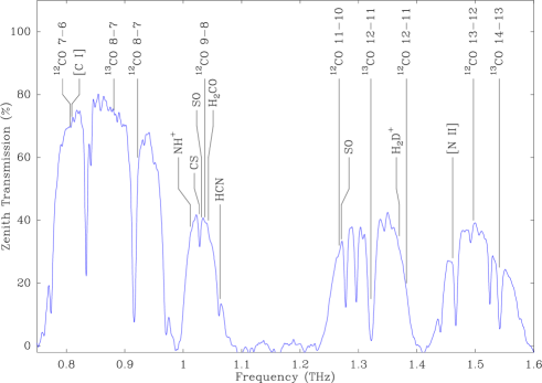
Figure 1: An example of the terahertz windows available from Cerro Sairecabur. This atmospheric transmission spectrum is actual data from the Receiver Lab Fourier-transform spectrometer (discussed briefly in §3.1, see also Paine et al. 2000), obtained on a very good day at the RLT site. The frequencies of several astronomically interesting lines are also plotted.

2 The Receiver Lab Telescope

The RLT is located on Cerro Sairecabur in northern Chile, 40 km north of the future ALMA site. This site, at a latitude of 22.5^∘ S, is well suited for studies of the inner galaxy and nearby spiral arms as most objects in these regions pass almost directly overhead. The telescope sits at an elevation of 5525 meters, 500 meters higher than ALMA, making it the highest telescope in the world. During the SAO site testing program that preceded the construction of the RLT, the Receiver Lab Fourier-transform spectrometer (FTS) was used at the ALMA site (Paine et al. 2000) and on Sairecabur. It was found that the Sairecabur site shows better peak transmission and a higher fraction of time available for terahertz observations because it is more often above the atmospheric inversion layer responsible for trapping moisture. An example of the transmission at Sairecabur is shown in Figure 1.

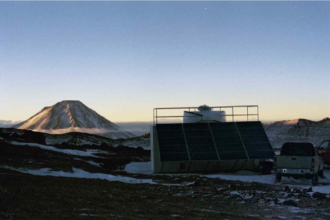
Figure 2: The Receiver Lab Telescope, on Cerro Sairecabur, Chile.

The RLT (Figure 2) is an 80 cm alt-az telescope sitting atop a 20-foot shipping container. The container houses the telescope tower, receivers, correlator, control computer, and equipment associated with the solar power system. The telescope is outfitted with two receivers for frequencies between 800 GHz and 1.6 THz. Frequency coverage is currently limited by the availability of solid state local oscillators, so the 1.5 THz window is not accessible. The mixers are waveguide-mounted phonon-cooled HEBs. All of those used on the telescope have been NbN devices, with and without MgO buffer layers. Typical noise temperatures are 950-2000 K in our frequency range. The 1 GHz wide IF is centered on 3 GHz. Spectra are obtained from a 330 channel digital autocorrelation spectrometer with 3 MHz resolution (1 km/s at 1 THz).

The RLT routinely observes spectral lines that are rarely, if ever, observed anywhere else. The most commonly used lines are ¹²CO $J=7\rightarrow 6$ (806.65 GHz), ¹³CO $J=8\rightarrow 7$ (881.27 GHz), and ¹²CO $J=9\rightarrow 8$ (1.03691 THz). With an 85^′′ beam at 1 THz, the RLT is well suited to mapping of extended emission, such as that arising in large H II regions. The first RLT terahertz spectrum was obtained on November 11, 2002. First scientific results can be seen in Marrone et al. (2004).

In the near future there are many upgrades planned for the telescope. In May we will begin observations of the CO $J=11\rightarrow 10$ line at 1.2670 THz, the first ground-based observations of this line. Expansion to the 1.5 THz window awaits a local oscillator, which should arrive this year. The correlator is due to be replaced with a new 512-channel correlator with 1 and 2 MHz resolution, providing greater detail in the narrow galactic emission lines we normally observe.

3 Challenges of Ground-based Terahertz Astronomy

Ground-based terahertz telescopes have some advantages over airborne or spaceborne instruments. Ground telescopes can be made larger than is feasible in the air or in space, are considerably cheaper, are easier to service than satellites, and may provide more observing time than can be obtained from an aircraft. Of course, observations from the ground are strongly limited by the properties of the atmosphere. Most importantly, observations are only possible in a few windows, but even within these windows the high atmospheric opacity, lack of strong calibrators, and the instabilities of terahertz receivers conspire to make common pointing, calibration, and telescope characterization tasks difficult. In the following sections we discuss solutions to these problems derived from 18 months of RLT operations.

3.1 Atmospheric Calibration

In order for spectra obtained from a terahertz telescope to be scientifically useful they must be properly calibrated. A common convention is to correct measured spectra for receiver gain, inefficiencies in the telescope, and atmospheric absorption, placing the observed line on a temperature scale that would be observed by a perfect telescope above the atmosphere (this is the $T^{*}_{A}$ scale of Ulich & Haas 1976). The atmospheric correction, and typically the efficiency correction, requires a reliable method of determining the opacity.

At the best well-characterized observing sites the atmospheric transmission in the windows above 1 THz is no better than $\sim 40$%, and is generally much lower. In addition, our experience at Cerro Sairecabur shows that large variations in transmission are common: in a single night the zenith transmission can vary by as much as 50% of its peak value. Changes in transmission between and within observing nights, whether due to changing source elevation or atmospheric fluctuations, can have a significant effect on the apparent strength of a spectral line. Without reproducible atmospheric correction, data taken on different nights, or even at different times in the same night, cannot be usefully compared.

There are several techniques for properly accounting for the atmospheric attenuation. Most radio astronomy calibration techniques have been developed at lower frequencies where the atmospheric effects are smaller and receivers are more sensitive and stable, making it difficult to apply them directly to observations with the RLT. One such example is the skydip, in which the sky temperature is measured as a function of elevation and the resulting curve is used to determine the mean atmospheric temperature and zenith opacity. Although the variation in sky temperature with elevation is small when the atmospheric transmission is low, it is still easily measurable with RLT receivers. The most significant problem we have encountered with this technique is that instabilities in the power output of the receiver are greatly magnified in skydips when atmospheric transmission is low.

The magnification of power instabilities by skydips can be understood from the equation for the antenna temperature ($T_{A}$) on blank sky. At elevation $\epsilon$, with receiver noise $T_{rx}$, mean atmospheric temperature $T_{atm}$, and zenith transmission $t$, the measured $T_{A}$ is:

$$T_{A}=T_{rx}+T_{sky}+T_{cmb}\hskip 4.3pt$$

$$\simeq T_{rx}+T_{atm}\left(1-t^{x}\right)$$ (1)

where $x=csc(\epsilon)$. The cosmic background term ($T_{cmb}$) has been dropped in the second line because the Rayleigh-Jeans brightness temperature of the CMB is vanishingly small at 1 THz. The transmission inferred from $T_{A}$ measured at one elevation (as a function of the usually unknown $T_{atm}$) can be found by rearranging equation 1:

$$t=\left(1-\frac{T_{A}-T_{rx}}{T_{atm}}\right)^{1/x}$$ (2)

Instabilities in the IF output power ($P_{A}$), whether they originate in the receiver or the atmosphere, correspond to changes in the measured $T_{A}$ because $T_{A}$$=KP_{A}$, where $K$ is a conversion factor between power and antenna temperature determined using hot and cold loads. Differentiating equation 2 with respect to $P_{A}$ and substituting for $T_{sky}$ (as in equation 1), we obtain:

$$\frac{\partial t}{\partial P_{A}}=\frac{-t}{xP_{A}}\left[\left(1+\frac{T_{rx}}{T_{atm}}\right)t^{-x}-1\right]$$ (3)

Ignoring all other error contributions, we can translate this equation into a relationship between the rms power fluctuations and the rms error on $t$. By noting that $T^{*}_{A}$ is proportional to $t^{-x}$, we can go directly to the fractional error ($\sigma_{T^{*}_{A}}/T^{*}_{A}$) in spectra calibrated using a single skydip transmission measurement for power fluctuations $\sigma_{P_{A}}/P_{A}$:

$$\frac{\sigma_{T^{*}_{A}}}{T^{*}_{A}}=\left[\left(1+\frac{T_{rx}}{T_{atm}}\right)t^{-x}-1\right]\frac{\sigma_{P_{A}}}{P_{A}}$$ (4)

In reality, one does not use a single measurement to determine both $t$ and $T_{atm}$. For a more typical 10 point skydip, using RLT values for $T_{rx}$ (1000 K), $T_{atm}$ (250 K), and $t$ for frequencies above 1 THz (20%), the random calibration error contributed by transmission measurement error is of the order of 15-20 times the power instabilities. A typical rms noise on the continuum power output of an RLT receiver is 0.5%, making this a significant cause of error in calibration.

Rather than the skydip method described here, we directly measure the zenith transmission using our FTS during all RLT observations. This instrument generates an atmospheric transmission spectrum from 300 to 3500 GHz at 3 GHz resolution every 10 minutes, and does not require any of the telescope observing time (as skydips would). An example of the reproducibility of the FTS calibration is shown in Figure 3. Despite an interval of an hour between two observations of the same object, during which time the transmission was observed to decrease from 22.5% to 19% (or 19% to 12.5% at the source elevation), the two calibrated spectra show very similar amplitude. More details about the use of an FTS in calibrating astronomical data, including refinements that can be made using atmospheric models, can be found in Paine & Blundell 2004.

Figure 3: An example of the results of our FTS calibration technique. Shown are two spectra of Orion KL in CO $J=9\rightarrow 8$ (1.037 THz), each required 1 minute of on-source integration time and the two observations were made one hour apart. The system temperature increased by 56% between the observations, but the difference between the two calibrated spectra is almost consistent with the rms noise seen in the baseline channels.

3.2 Telescope Characterization

The RLT has also faced difficulties in determining the telescope efficiency, beamshape, and radio pointing. Typically, these properties would all be measured by mapping the continuum emission of a planet, but we have found that drifts in the power output of our HEB receivers make continuum maps unreliable.

An alternative approach is to use a more narrowband signal as a calibration source, since other noise sources should be less important relative to radiometric noise in a smaller bandwidth (e.g. Schieder & Kramer 2001). Narrow, unsaturated atmospheric lines, such as O₃ lines, provide exactly such a signal when observed against the disk of a planet. Moreover, by using planets as a backlight we retain the source geometry that is normally used for these purposes.

Our procedure for obtaining a beam map, pointing offsets, and a beam efficiency is as follows. We make a map of a planet using an ozone line near to the observing frequency of interest. Once calibrated, we fit each spectrum in the map with a model ozone line profile to determine a best-fit line depth. The line depths form the basis for a beam map because the variations in line depth reflect changes in the coupling of the telescope beam to the planet (rather than an atmospheric effect), just as continuum measurements would. By fitting the derived map we obtain a beamshape and an offset from the nominal source position. The fit also yields the line depth that would be observed if there were no pointing error, which, after accounting for the coupling of the beam to the planet, can be used to determine the efficiency.

Our method and the standard continuum method are similar in many respects. We require good calibration to ensure that the individual map spectra can be reliably compared to each other, but this is no different than what is required for a continuum map taken over a long enough interval that the atmospheric transmission and source elevation change. Once the calibrated line depths are obtained, the procedures for determining the pointing and beam shape are the same as one would use with a continuum map. The only additional requirement of this portion of our method is a model ozone lineshape, which we obtain from the am atmospheric model (Paine 2004) and a vertical ozone profile from ozonesonde and lidar observations made from Hawaii (Oltmans et al. 1996, Leblanc & McDermid 2000). The line depths we determine are only weakly dependent on the assumed vertical ozone profile for reasonable profiles. For the efficiency determination we need a good estimate of the true strength of the ozone absorption. The absorption represents the known signal to which we compare our observed signal and obtain an efficiency, analogous to comparing a measured continuum brightness temperature to an expected planetary brightness temperature. Fortunately, the total O₃ column is measured daily at many sites worldwide, including the nearby Marcapomacocha, Peru, and is made available by the NOAA Climate Monitoring and Diagnostics Laboratory.

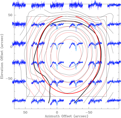
Figure 4: An O₃ beam map made with the RLT against Jupiter. Spectra were taken on a 30^′′ grid in an irregular order to reduce the biasing effects of calibration errors. The individual spectra ( —–) and best fit line profiles ( —–) are shown at each map point. The absorption at the left edge of each spectrum is a correlator artifact. The beam is fit to the central 16 spectra (enclosed in a box). The measured (—–) and best fit ( —–) beams are contoured in 10% steps with the 50% contour reinforced. The two contour sets are seen to agree well over most of the map, except toward the north where noisy spectra that have been excluded from the fit cause the measured contours to deviate from the best fit contours.

Figure 4 is an example of a beam map made with the technique just described. The map was made using the 883.057 GHz line of ozone, with Jupiter (41.7^′′ diameter) as the continuum source. From this map we find pointing offsets of -19.0$\pm$1.6^′′ and -12.4$\pm$2.1^′′ and FWHM beamsizes of 96$\pm$5^′′ and 117$\pm$9^′′ in azimuth and elevation, respectively, along with a line depth of 5.3$\pm$0.3 K, which corresponds to an efficiency of 44%. The measured pointing offsets are small compared to the beamsize and are comparable to those suggested by previous terahertz observations. The beamsize is similar to what is expected from the optics design, while the efficiency suggests that at the time that this map was made the receiver was shifted slightly from the designed position so that its beam was clipped before reaching the telescope.

We believe that the use of ozone lines as a calibration tool can also be extended to other telescopes. To determine whether this is a useful technique at a given telescope one must compare the fluctuations in the receiver output power, scaled by the system temperature, to the signal strength from available planets. For the RLT and Jupiter, the expected signal is around 10 K at 1 THz, but the receiver instabilities (of the order of 0.5% rms in 1 second integrations on the RLT) applied to a $T_{sys}$ of 20000 K correspond to 100 K fluctuations. Larger telescopes see a larger planetary signal, so they may be able to tolerate small instabilities. On the other hand, if beam maps are made in poorer transmission or at lower source elevation $T_{sys}$ can be significantly larger than the 20000 K used here. The use of ozone as a calibrator is not something that restricts this technique to Chile; daily ozone measurements are also made from Mauna Loa, Hawaii, and the South Pole, so this information is available for all major submillimeter sites. This technique can be used near to any frequency of interest because suitable ozone lines are available throughout all of the terahertz windows. As a final consideration, the measurement technique employed in making the beam map may affect the expected depth of the ozone line. For position- or beam-switched observations, where the map spectra are obtained by combining on- and off-source spectra as (ON-OFF)/OFF, the expected line depth is not simply proportional to the planet signal times the fractional absorption due to ozone. As $T_{rx}$ decreases, a term in the expansion of the line depth that is insignificant for the RLT ($<$5% for $T_{rx}+T_{sky}=1200$ K) grows like $1/\left(T_{rx}+T_{sky}\right)$ and could be relevant for lower noise terahertz receivers.

4 Conclusions

We have discussed the status of the SAO Receiver Lab Telescope, presently the only telescope making ground-based astronomical observations at frequencies above 1 THz. We are currently beginning observations in the 1.3 THz atmospheric window, while observations in the 1.5 THz window await a local oscillator. Neither of these windows has previously been used for astronomical observations.

We have also presented techniques for making ground-based terahertz observations. In particular, we have discussed the difficulty of using skydips for data calibration and the power of a Fourier-transform spectrometer as a calibration tool. We have also presented a new technique for characterizing a telescope in the presence of high system temperatures and receiver instabilities.

References

Blundell, R. et al. 2002, in Proc. Thirteenth International Symposium on Space Terahertz Technology

Gerecht, E. et al. 2003, in Proc. Fourteenth International Symposium on Space Terahertz Technology

Leblanc, T. & McDermid, I. S. 2000, Journal of Geophysical Research, 105, 14613

Marrone, D. P., et al. 2004, Astrophysical Journal in press (astro-ph/0405530)

Matsushita, S., et al. 2000, in Proc. SPIE Vol. 4015, Radio Telescopes, ed. H. R. Butcher, 378-389

Nikola, T, et al. 2004, these proceedings

Oltmans, S. J. et al. 1996, Journal of Geophysical Research, 101, 14569

Paine, S. et al. 2000, Publications of the Astronomical Society of the Pacific, 112, 108

Paine, S. 2004, “The am Atmospheric Model” SMA Technical Memo #152, available at
http://sma-www.cfa.harvard.edu/private/memos

Paine, S. & Blundell, R. 2004, these proceedings

Radford, S. J. E., et al. 2003, in Proc. Fourteenth International Symposium on Space Terahertz Technology

Schieder, R. & Kramer, C. 2001, Astronomy & Astrophysics, 373, 746

Stark, A. A. et al. 2001, Publications of the Astronomical Society of the Pacific, 113, 567

Ulich, B. L. & Haas, R. W. 1976, Astrophysical Journal Supplement Series, 30, 247