Observational manifestations of solar magneto-convection — center-to-limb variation

Abstract

We present the first center-to-limb G-band images synthesized from high resolution simulations of solar magneto-convection. Towards the limb the simulations show “hilly” granulation with dark bands on the far side, bright granulation walls and striated faculae, similar to observations. At disk center G-band bright points are flanked by dark lanes. The increased brightness in magnetic elements is due to their lower density compared with the surrounding intergranular medium. One thus sees deeper layers where the temperature is higher. At a given geometric height, the magnetic elements are cooler than the surrounding medium. In the G-band, the contrast is further increased by the destruction of CH in the low density magnetic elements. The optical depth unity surface is very corrugated. Bright granules have their continuum optical depth unity 80 km above the mean surface, the magnetic elements 200-300 km below. The horizontal temperature gradient is especially large next to flux concentrations. When viewed at an angle, the deep magnetic elements optical surface is hidden by the granules and the bright points are no longer visible, except where the “magnetic valleys” are aligned with the line of sight. Towards the limb, the low density in the strong magnetic elements causes unit line-of-sight optical depth to occur deeper in the granule walls behind than for rays not going through magnetic elements and variations in the field strength produce a striated appearance in the bright granule walls.

1 Introduction

G-band filtergram bright points are commonly used as proxies for small scale magnetic flux concentrations, sometimes called “flux tubes”, (Muller & Roudier, 1984; Berger et al., 1995; Berger & Title, 2001), although it is known that not all magnetic elements are associated with bright points (Berger & Title, 1996). Such bright points are also observed in the photospheric continuum, but with lower contrast (Dunn & Zirker, 1973). The reason for this association is the decreased opacity in the magnetic concentration (Kiselman et al., 2001; Rutten et al., 2001; Sánchez Almeida et al., 2001; Steiner et al., 2001; Uitenbroek, 2003; Keller et al., 2004). The primary reason for the lower opacity is the lower density in magnetic concentrations, which maintain rough pressure equilibrium with their surroundings. The contrast in the G-band is increased by the destruction of the CH molecules, again due to the low density, although some have also cited increased temperatures as a cause (Schüssler et al., 2003; Sánchez Almeida et al., 2001; Steiner et al., 2001). Towards the limb magnetic concentrations are visible as bright faculae, where one sees the hot granule walls behind the low opacity magnetic concentrations (Spruit, 1976, 1977; Lites et al., 2004; Keller et al., 2004).

Here we examine the variation in the appearance of the G-band from disk center toward the limb using images calculated from a solar magneto-convection simulation.

2 Methods

The 3D magneto-convection simulations include LTE ionization and excitation in the equation of state, and non-grey, LTE radiation transfer in the energy balance. They cover a small region of 6 $\times$ 6 Mm, sufficient to include one meso-granule and many granules, and extend from the temperature minimum down to a depth of 2.5 Mm below $<\tau_{\mbox{500}}>=1$. The resolution is 25 km horizontally and varies from 15 km in the upper layers to 35 km vertically in the lower layers (Stein & Nordlund, 1998). The simulation is started with a uniform vertical magnetic field of 250 G superimposed on a snapshot of non-magnetic convection and then allowed to relax. The magnetic field is quickly swept to the boundaries of the deep lying mesogranules and concentrated to typical strengths 1.7 kG at the level $<\tau_{\mbox{500}}>=1$.

The emergent spectrum was calculated in LTE in two wavelength intervals of 3 nm width centered on 430.68 nm (G-band) and 436.52 nm (G-continuum) (all wavelengths given as vacuum wavelengths). Molecular equilibrium was calculated including all di-atomic molecules of hydrogen, carbon, nitrogen and oxygen. In each wavelength band, 1364 frequency points were used for the spectrum calculation. Line opacities from 21 atomic species and molecular lines from CH were included with data from Kurucz & Bell (1995) and Kurucz (1993). Depth-dependent Voigt profiles were used for all lines. In total 1838 lines were considered. The calculated emergent intensities were multiplied with filter transmission curves from the Swedish 1-meter Solar Telescope filters with central wavelengths as above and FWHM of 1.08 nm (G-band) and 1.15 nm (G-continuum) and integrated over wavelength to create synthetic images in the G-band and G-continuum.

3 Simulated Observations

We investigate the response of the G-band and G-continuum to magnetic concentrations, the so-called “flux tubes”, at disk center and towards the limb. We consider disk center first.

3.1 Disk Center

Hydrodynamic calculations using the same code have previously been checked by comparing simulated and observed iron line profiles (Asplund et al., 2000). The accuracy of both the current simulation and the G-band calculation was checked by comparing the spatially averaged G-band spectrum calculated from a simulation snapshot with observations. The simulated G-band spectrum calculated without any micro- or macro-turbulence or extra wing damping is in excellent agreement with the Jungfraujoch atlas (Delbouille et al., 1989), with only a 8% rms difference between the two. These tests verify the realism of the simulation and the accuracy of the G-band calculation.

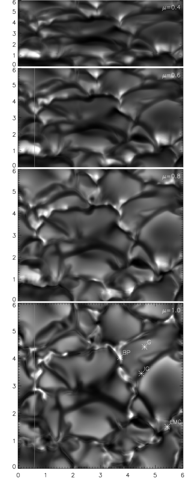
Figure 1: G-band images at disk center and $\mu=0.8,0.6,0.4$. The bright line shows the slice along which we show the atmospheric structure and location of peak emission. Axes are distances in Mm. The panels have individual scalings. Points marked G, IG, BP and LMC refer to the locations where the temperature stratification is shown in figure 4.

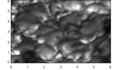
Figure 2: Observed G-band intensity from the Swedish 1-m Solar Telescope at $\mu=0.63$. Data processing done by Luc Rouppe van der Voort.

Figure 1 shows the G-band images at $\mu$ = 1.0, 0.8, 0.6 and 0.4 for a snapshot from our simulation. The appearance is very similar in its general properties to observed images (Fig. 2). Our average field strength of 250 G is more like a plage region, but the appearance is more like the quiet Sun. With higher spatial resolution in the simulations the same appearance would occur for smaller average fields, because the simulations would then allow compression to smaller scales. The same typical field strengths of 1.7 kG would then occur but in structures of smaller spatial extent.

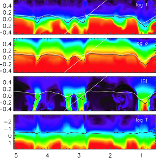
Figure 3: Temperature, density and magnetic field strength along a vertical slice through magnetic and non-magnetic regions, with the average formation height for the G-band intensity for a vertical ray (black line) and at $\mu=0.6$ (white line). One ray at $\mu=0.6$ is also shown in white. Axes are distances in Mm. The bottom panel shows temperature as function of lg $\tau_{500}$.

The magnetic concentrations are partially evacuated and cooler than their surroundings at a given geometric layer, and in approximate pressure equilibrium with the surrounding non-magnetic plasma (Fig. 3). Because they are cooler and less dense, the layer from which radiation emerges lies deeper, often sufficiently deep that the temperature is higher than at the formation height in non-magnetic granules (Fig. 4). The $\tau_{500}$=1 surface is extremely corrugated, ranging from 97 km above (in granules) to 323 km below (Wilson depression) the average. Higher temperatures at $\tau_{500}$=1 are due to radiative heating from the hot walls of the magnetic concentrations as predicted by Spruit (1977, 1976). Indeed, in calculations where horizontal radiative transfer is omitted, these higher temperatures at $\tau_{500}$=1 are absent, confirming the role of radiative heating from hot side walls. As a result of this heating, the magnetic concentrations often appear as bright points in the intergranular lanes. This is especially apparent in the G-band, where the contrast is enhanced because CH is destroyed in the low density magnetic concentrations. All such bright points are associated with strong magnetic fields. However, there are significant numbers of locations of similar strong field that are not associated with G-band brightness at disk center (e.g. fig. 1 lower right and left). Whether a concentration appears bright or dark depends on its size – larger concentrations tend to be dark while smaller ones tend to be bright (Spruit, 1977).

Figure 4: Temperature vs. height for four locations: G=granule, IG=intergranular lane, BP=magnetic bright point, LMC=large magnetic flux concentration. Stars are mean formation height of the G-band and pluses of the G-continuum. Magnetic flux concentrations are cooler than their surroundings at a given geometric height but their radiation emerges from deeper, hotter layers.

The bottom panel of Fig 3 shows the temperature as function of lg $\tau_{500}$. The contrast in temperature between magnetic concentrations and non-magnetic areas increases with decreasing optical depth giving larger intensity contrast with increasing opacity (e.g. Ca H,K). The G-band has its mean formation height (black line in bottom panel) at lg $\tau_{500}$=-0.48 corresponding to a mean formation height 54 km above where $\tau_{500}$=1, therefore giving a larger contrast than in the continuum. The contrast enhancement by the destruction of CH is seen as a dip in the curve showing the mean formation optical depth in the bottom panel. Note also that the G-band intensity has its peak contribution at similar heights as the continuum (that’s why the granulation pattern looks similar) but the many spectral lines give a broad tail of the contribution function to higher layers. This causes a more “fuzzy” image than the sharper contribution function from a monochromatic diagnostic would give.

One often sees especially dark lanes along the sides of the G-band bright points. These are the cool intergranular downflows that have been excluded from the magnetic concentrations. In addition, near the layer of $<\tau_{500}>=1$, the magnetic concentrations are surrounded by rings of slightly lower temperature where the magnetic field strength gradient is largest.

Finally, while most of the granulation appears normal, where there is a wide, strong magnetic field concentration along the bottom edge of the image, the granulation appears very disturbed, with lots of small, irregular bright and dark features.

3.2 Center to Limb Variation

As one observes towards the limb several differences in the surface appearance occur (Fig. 1). First, the granules develop a three-dimensional pillow appearance with the granules higher than the intergranular lanes, and their near sides brighter than their far sides. This is partly due to the true three-dimensional structure of granulation with the granules observed higher than the intergranular lanes. Partly it is due to the near side being seen more normal to the line of sight and the far side at a more glancing angle. Finally, this is enhanced by the magnetic concentrations, which because of their low density and resulting low opacity allow one to see deeper into the hot granules behind them (the “hot wall” effect (Spruit, 1977, 1976; Keller et al., 2004)). This is further enhanced by the occurrence of the largest horizontal temperature gradients along the boundaries of some of the magnetic concentrations. These features are illustrated in the figure 3 which show the temperature, density, magnetic field strength and the mean formation height of the G-band intensity for both a vertical line of sight and one at $\mu=0.6$, in a vertical slice through the simulation domain (location shown in fig. 1 as light vertical line). Note that the mean formation height for a slanted ray is more constant than for a vertical ray. The deep, low density magnetic concentrations get hidden by the fact that the ray goes through higher density material above the neighboring granule.

In figure 1 the bright faculae on the left and right sides near the bottom (at $\mu=0.8,0.6$) are behind the largest flux concentration at this time, which appear mostly dark in the disk center image. As one looks further toward the limb some of the faculae (especially in the upper part of the image) disappear because they lie deep in the intergranular lanes and become hidden behind the higher intervening granule tops. Where, however, the bright walls are viewed along an intergranular lane or where the magnetic concentration is sufficiently wide they remain clearly visible.

Another common phenomenon in observations and the simulated images is the appearance of striations in the bright granule walls. These striations are caused by variations in the magnetic field strength in front of the hot granule walls. Where the field is weaker, the density is higher, so the opacity larger. This effect is enhanced by a higher CH concentration also due to the higher density. Thus, where the magnetic field is weaker, the radiation emerges from higher, cooler layers, so these locations appear darker.

References

- Asplund et al. (2000) Asplund, M., Nordlund, Å., Trampedach, R., Allende Prieto, C., Stein, R. F. 2000, A&A, 359, 729
- Berger et al. (1995) Berger, T. E., Schrijver, C. J., Shine, R. A., Tarbell, T. D., Title, A. M., Scharmer, G. 1995, ApJ, 454, 531
- Berger & Title (1996) Berger, T. E., Title, A. M. 1996, ApJ, 463, 365
- Berger & Title (2001) Berger, T. E., Title, A. M. 2001, ApJ, 553, 449
- Delbouille et al. (1989) Delbouille, L., Roland, G., Neven, L. 1989, Atlas photometrique DU spectre solaire de [lambda] 3000 a [lambda] 10000. Vol.2, Liege: Universite de Liege, Institut d’Astrophysique, 1989
- Dunn & Zirker (1973) Dunn, R. B., Zirker, J. B. 1973, Sol. Phys., 33, 281
- Keller et al. (2004) Keller, C. U., Schüssler, M., Vögler, A., Zakharov, V. 2004, ApJ, 607, L59
- Kiselman et al. (2001) Kiselman, D., Rutten, R. J., Plez, B. 2001, in P.Brekke, B.Fleck, J.B.Gurman (eds.), Proceedings of IAU Symposium 203, p. 287
- Kurucz (1993) Kurucz, R. 1993, SYNTHE Spectrum Synthesis Programs and Line Data. Kurucz CD-ROM N o. 18. Cambridge, Mass.: Smithsonian Astrophysical Observatory, 1993., 18
- Kurucz & Bell (1995) Kurucz, R., Bell, B. 1995, Atomic Line Data (R.L. Kurucz and B. Bell) Kurucz CD-ROM No. 23. Cambridge, Mass.: Smithsonian Astrophysical Observatory, 1995., 23
- Lites et al. (2004) Lites, B. W., Scharmer, G. B., Berger, T. E., Title, A. M. 2004, Sol. Phys., in press
- Muller & Roudier (1984) Muller, R., Roudier, T. 1984, Sol. Phys., 94, 33
- Rutten et al. (2001) Rutten, R. J., Kiselman, D., Rouppe van der Voort, L., Plez, B. 2001, in M.Sigwarth (ed.), ASP Conf. Ser. 236: Advanced Solar Polarimetry – Theory, Observation, and Instrumentation, p. 445
- Sánchez Almeida et al. (2001) Sánchez Almeida, J., Asensio Ramos, A., Trujillo Bueno, J., Cernicharo, J. 2001, ApJ, 555, 978
- Schüssler et al. (2003) Schüssler, M., Shelyag, S., Berdyugina, S., Vögler, A., Solanki, S. K. 2003, ApJ, 597, L173
- Spruit (1976) Spruit, H. C. 1976, Sol. Phys., 50, 269
- Spruit (1977) Spruit, H. C. 1977, Sol. Phys., 55, 3
- Stein & Nordlund (1998) Stein, R. F., Nordlund, A. 1998, ApJ, 499, 914
- Steiner et al. (2001) Steiner, O., Hauschildt, P. H., Bruls, J. 2001, A&A, 372, L13
- Uitenbroek (2003) Uitenbroek, H. 2003, in A.A.Pevtsov, H.Uitenbroek (eds.), ASP Conf. Ser. 286: Current Theoretical Models and Future High Resolution Solar Observations: Preparing for ATST, p. 403